Sage Journals: Discover world-class research

Abstract

Growing awareness of how susceptible research is to errors, coupled with well-documented replication failures, has caused psychological researchers to move toward open science and reproducible research. In this Tutorial, to facilitate reproducible psychological research, we present a tool that creates reproducible tables that follow the American Psychological Association’s (APA’s) style. Our tool, apaTables, automates the creation of APA-style tables for commonly used statistics and analyses in psychological research: correlations, multiple regressions (with and without blocks), standardized mean differences, N-way independent-groups analyses of variance (ANOVAs), within-subjects ANOVAs, and mixed-design ANOVAs. All tables are saved as Microsoft Word documents, so they can be readily incorporated into manuscripts without manual formatting or transcription of values.

Keywords

R replication reproducibility open science statistical tools transparency in research open data data sharing reproducible research reproducible tables reproducible analyses open materials

The growing awareness of errors in research (e.g., John, Loewenstein, & Prelec, 2012; Nuijten, Hartgerink, van Assen, Epskamp, & Wicherts, 2016; Stanley & Spence, 2014), coupled with high rates of replication failures (Open Science Collaboration, 2012, 2015), has generated calls for change and recommendations for restructuring how research is conducted and evaluated (Nosek et al., 2015; Pashler & Wagenmakers, 2012). One approach, open science, encourages the preregistration of analysis plans (see http://aspredicted.org and http://osf.io) as well as the posting of materials and analysis code in open-access repositories (Nosek et al., 2015). One aim of open science is to create reproducible research. The term reproducible research has been used in various ways, but many researchers use it to refer to research whose results can be reproduced using the same data, code, or both as the original authors used (Peng, 2011). Published articles with reproducible results are becoming increasingly common in fields such as computer science (Ince, Hatton, & Graham-Cumming, 2012), biostatistics (Peng, 2009), medicine (Laine, Goodman, Griswold, & Sox, 2007), epidemiology (Peng, Dominici, & Zeger, 2006), and econometrics (Koenker & Zeileis, 2009). Interest in reproducible research is also increasing in psychology (e.g., Winerman, 2017).

Because the general aim of reproducible research is for other researchers to be able to re-create and verify methods, results, and documents, reproducibility encompasses many aspects of the scientific process. One important aspect of the scientific process is the creation of tables that communicate results efficiently (e.g., Peng et al., 2006). For a piece of scholarship to be reproducible, its associated tables also need to be reproducible from the data. Generating reproducible tables is not trivial, as tables are often created and formatted manually, with values individually transcribed into their respective cells by researchers. Not surprisingly, creating, formatting, and transcribing values into tables can be a tedious and potentially error-prone process. Some typographical errors may be trivial, but others may have the potential to alter the interpretation of and conclusion drawn from results. For instance, a recent investigation revealed that reporting errors are widespread in the text of psychology articles (Nuijten et al., 2016). Specifically, a review of 16,695 articles drawn from eight major journals between 1985 and 2013 revealed that 49.6% of the articles reporting null-hypothesis significance testing had at least one p value that was inconsistent with the test statistic, and 12.9% of the articles had an inconsistency that was large enough to change a statistical conclusion (p. 1209).

Moreover, when creating tables, psychological researchers often need to comply with a specific formatting style that is set by the American Psychological Association’s (APA’s) style guide (APA, 2010). These style requirements can create tedious work for researchers, who may have to repeatedly copy and paste, align table entries, and fit and refit contents to create a table that satisfies APA guidelines and also presents the necessary statistical information. In this Tutorial, we present a tool that automates the creation of properly formatted APA-style tables for several commonly used statistics and analyses in psychology: correlations, multiple regressions (with and without blocks), standardized mean differences, N-way independent-groups analyses of variance (ANOVAs), and within-subjects and mixed-design ANOVAs. Our tool, apaTables, is available as a free package for the R software environment (R Core Team, 2018).

Disclosures

The code for all the examples in this Tutorial is available on the Open Science Framework at https://osf.io/jsvdz. The code for apaTables is available on GitHub at this link: https://github.com/dstanley4/apaTables.

The apaTables Package

The apaTables package is designed to automate the generation of properly formatted APA-style tables for several commonly used analyses in psychology. All tables are created in Microsoft Word format, which makes it easy for users to include them in manuscripts. In addition to making it simple and easy to create APA-style tables, our package has features that facilitate data analyses.

It is not uncommon for it to be necessary to run several different analyses to obtain all of the statistics needed for an APA-style table. For example, in the case of a correlation table, the means and standard deviations can be computed with one command, the correlations with another, and confidence intervals (CIs) for correlations with yet another. Likewise, when a regression is conducted using the lm command, the unstandardized regression weights (i.e., b weights) are generated, and then an additional command is needed to obtain standardized weights (i.e., β weights). Similarly, with ANOVAs, after the lm (or aov) command is run, additional steps are required to obtain Type III sums of squares and effect sizes. Our software package allows users to use simple R code to create properly formatted APA-style tables with all the necessary statistics.

A variety of software options are available to create reproducible documents. A reproducible document is one that is created dynamically by weaving together manuscript text, analysis scripts, and data. In the final document, the numbers in the text and tables are not entered by hand, but rather are inserted by the script that conducted the analyses. Many researchers use the rmarkdown package for R to create reproducible documents (see Kuhn, 2018). However, tables with the nuanced formatting required for APA style cannot be created for the Microsoft Word format using rmarkdown because of current limitations of the software systems that underlie it. Consequently, our package directly creates a .doc file based on user inputs. There are a number of R packages that can be used to create and export tables (e.g., huxtable—Hugh-Jones, 2018; xtable—Dahl, 2016; ascii—Hajage, 2011; htmlTable—Gordon, Gragg, & Konings, 2018; papaja—Aust & Barth, 2018). An advantage of these other packages is that they are flexible and allow users autonomy in formatting (e.g., borders, alignment, background color) and output options (e.g., html, LaTeX). The aim of apaTables, however, is to streamline the creation of reproducible tables by automating formatting decisions to comply with APA standards. This way, users are not required to do any manual formatting. As a result, apaTables intentionally does not provide the same level of flexibility as other table packages.

An additional feature of our package is that it calculates effect sizes and confidence intervals and reports them in tables when possible. This is a particularly valuable feature, as many researchers rely solely on p values when interpreting and reporting results, an approach that has been widely criticized. For example, the American Statistical Association (ASA, 2016) recently released a position paper on the use of p values in research. One of the six principles advocated in that statement was that “scientific conclusions and business or policy decisions should not be based only on whether a p-value passes a specific threshold” (p. 2). The executive director of the ASA (R. Wasserstein) has suggested that effect sizes with confidence intervals should be used to interpret data (Retraction Watch, 2016, para. 21). This position is also consistent with recommendations of the APA Task Force on Statistical Inference (see Leland & Task Force on Statistical Inference, 1999).

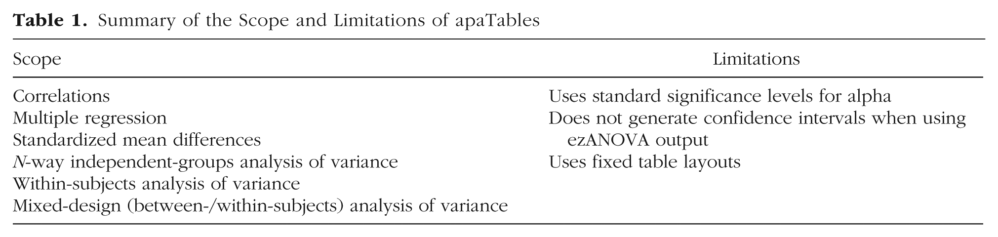
In the following sections, we illustrate how the apaTables package can be used to construct tables for a variety of analysis techniques that are commonly used in psychology. Because apaTables is an open-source package, users are free to use it as they like. However, in the context of other R code, users may find it helpful to situate the apaTables package after R code that preprocesses data and conducts primary analyses. A summary of the scope and limitations of apaTables is presented in Table 1.

Table 1.

Summary of the Scope and Limitations of apaTables

Scope	Limitations
CorrelationsMultiple regressionStandardized mean differencesN-way independent-groups analysis of varianceWithin-subjects analysis of varianceMixed-design (between-/within-subjects) analysis of variance	Uses standard significance levels for alphaDoes not generate confidence intervals when using ezANOVA outputUses fixed table layouts

Learning Objectives and Assumed Knowledge

The objectives of this Tutorial are to teach readers how to use the apaTables package to generate APA-style tables for correlations, multiple regressions (with and without blocks), standardized mean differences, N-way independent-groups ANOVAs, and within-subjects and mixed-design ANOVAs. By working through the Tutorial, readers will learn how to install packages, run analyses, and create and view tables. A basic working knowledge of R and RStudio is helpful, but not required. We have structured the Tutorial so that both novices and experts will benefit. Those who are comfortable with R may want to skip this section and go directly to the section describing how to create correlation tables.

Installation of R and RStudio

To use apaTables, researchers need to download and install R (R Core Team, 2018). This is a free download, available at https://www.r-project.org. Additionally, we suggest that RStudio be downloaded and installed. RStudio is also a free download, and it is available at https://www.rstudio.com. Once RStudio is installed, it is not ever necessary to open R; only RStudio should be used to access R commands. We opted to use RStudio in this Tutorial because it makes R substantially easier for novices to use, though strictly speaking, it is not needed. The commands used in this Tutorial should be typed into the Console window within RStudio.

Installation of R packages

One concept that new R users may struggle with is that R is supplemented by a large number (more than 10,000) of user-created packages that are located on CRAN. It may help to consider packages as analogous to smartphone apps.¹ That is, using the install.packages command is similar to downloading an app from the App Store and installing it on a smart device. Using the library command in R is similar to opening an app that has been downloaded (Table 2).

Table 2.

Correspondence Between the Terminologies Used for R Packages and Smartphones

R terminology	Smartphone terminology
CRAN	App Store
Package	App
install.packages	Download app from App Store
library	Open app

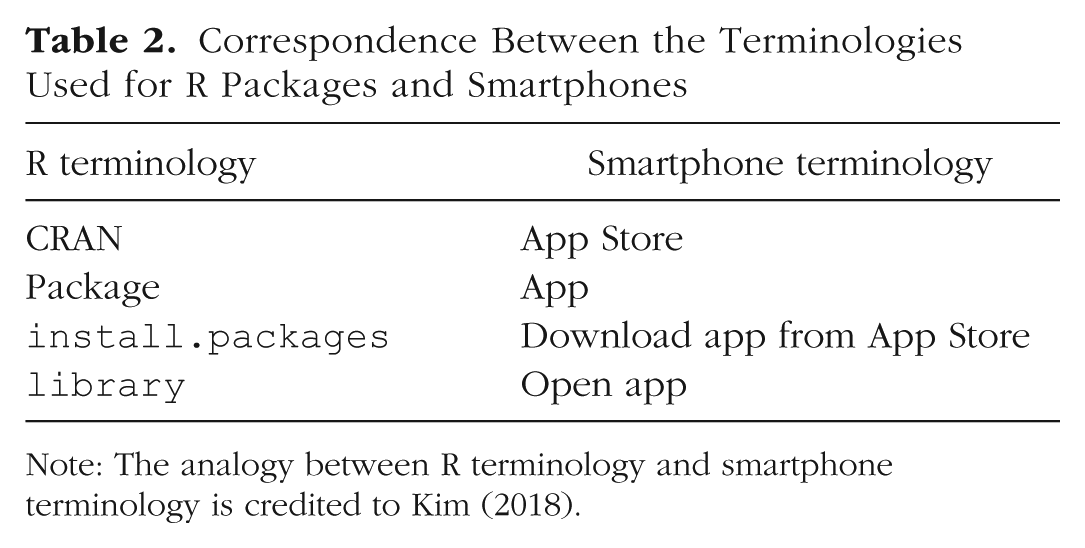
Note: The analogy between R terminology and smartphone terminology is credited to Kim (2018).

To follow this Tutorial, you will need to download apaTables from CRAN. This can be done with the following command:

install.packages(“apaTables”, dependencies = TRUE)

Note that in this command, we have indicated that dependencies is equal to TRUE. This ensures that any other packages used by apaTables are also downloaded and installed.

To follow this Tutorial, you will also need to download and install a collection of packages known as the tidyverse (Wickham, 2017). The tidyverse approach to using R is generally considered easier for novices than older base R techniques, though some more experienced R users still prefer those older techniques. In order to use the repeated measures and mixed-design ANOVA functions, you will need to install, the ez package (Lawrence, 2016), which makes running within-subjects analyses in R much simpler. To install these two packages, use these commands:

install.packages(“tidyverse”, dependencies = TRUE)

install.packages(“ez”, dependencies = TRUE)

Note that packages need to be installed only once, in the same way that an app needs to be downloaded to a smartphone only once. You may open an app innumerable times using the library command. Although we include the library command in explaining how to create tables for each type of analysis discussed in this Tutorial, readers need to install packages only once as they work through the examples.

Suggested workflow: RStudio projects

A problem that can be encountered when starting to use R is remembering to specify the working directory, that is, the location from which files are loaded and to which they are saved. If the working directory is not correctly specified, users can encounter errors when loading data files and when trying to locate saved files (e.g., tables). We have found that it is not uncommon for users who are new to R to forget to specify the directory or to mismanage it if they are doing this manually. Consequently, we recommend using projects within RStudio to avoid the pitfalls associated with manually specifying the working directory. More specifically, with projects, R will always use your project directory to load and save files. You do not ever have to manually specify the working directory within R.

Projects are easy to use and map onto the typical workflow associated with data analyses conducted with traditional statistical software. Begin by creating a directory, or folder, into which you will put your data files. For our examples, we will use a directory called MyResearchProject. Once this folder has been created, drag the data files you wish to analyze into this folder. For example, if you want to use an SPSS data file called study1.sav, simply place this file in the MyResearchProject directory.

Next, tell RStudio to treat this directory as a project. To do so, open RStudio and select the “New Project” option in the “File” drop-down menu. Once “New Project” is selected, a window will appear (Fig. 1). Choose the “Existing Directory” option. The next step is to indicate the directory that you previously created and stored your data in. Use the “Browse” button to tell RStudio where this directory is located (see Fig. 2).

Fig. 1.

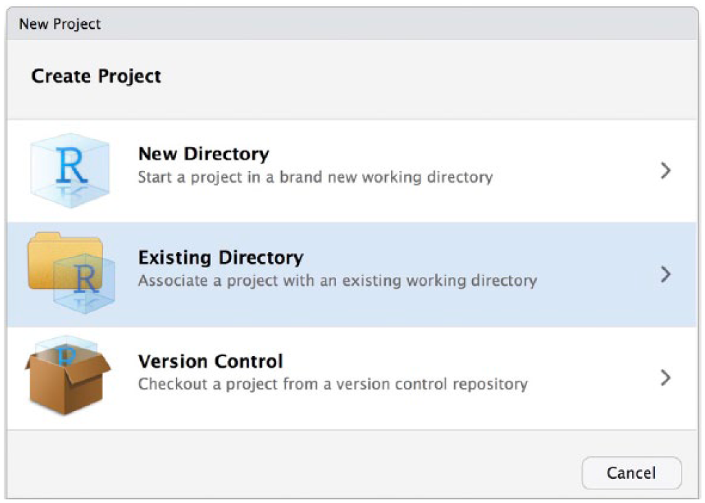
Screenshot of the RStudio window where users can specify that the project they are creating is an existing directory.

Fig. 2.

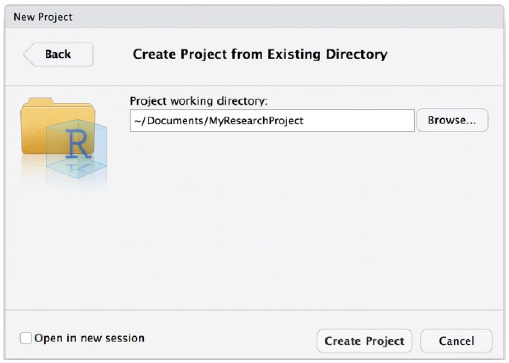
Screenshot showing the RStudio window with the “Browse” button, which can be used to specify the project directory.

Once you have specified your project directory, click the “Create Project” button at the bottom of the window. This will create a file that ends with .Rproj in your project directory (in our example, this file is called MyResearchProject.Rproj). This file can then be seen in the File panel in the lower right corner of RStudio (see Fig. 3).

Fig. 3.

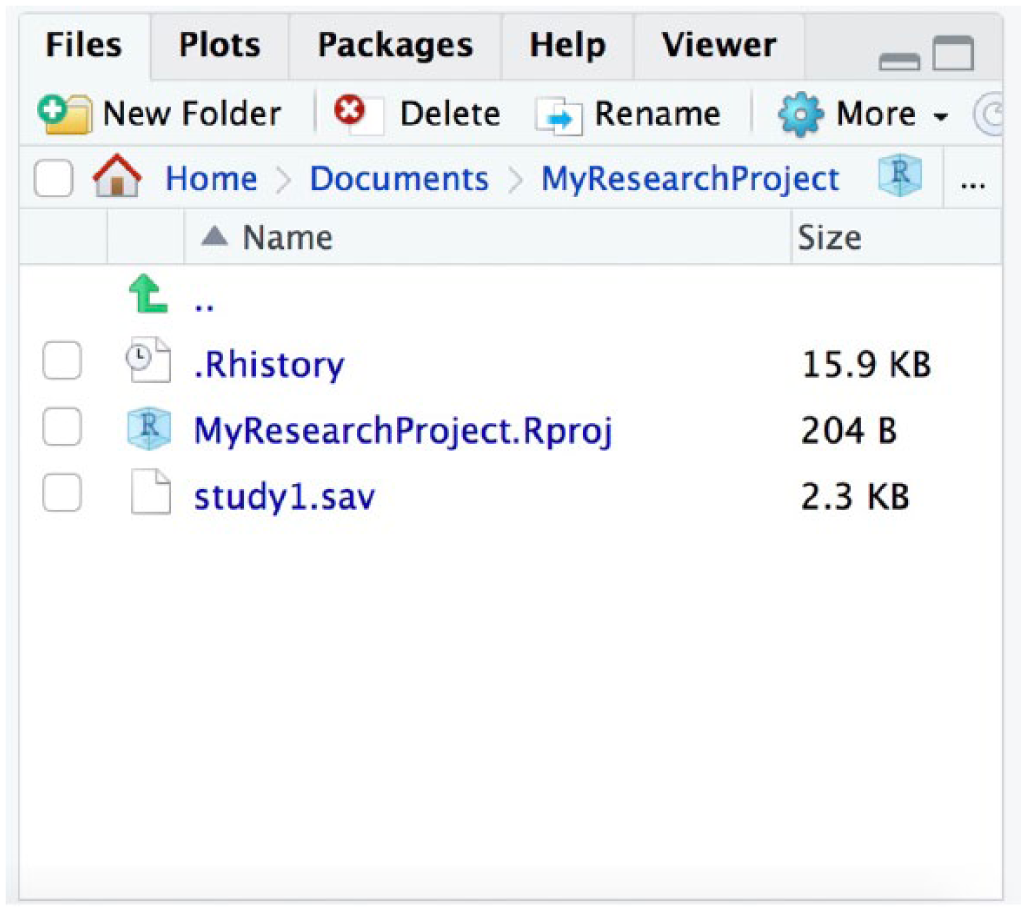
Screenshot showing the File panel in RStudio after MyResearchProject has been specified as a project directory.

Now that RStudio considers this a project directory, you do not need to worry about the path to the directory when you refer to a file in it. For example, you can simply load study1.sav by referring to the file name in quotes without providing RStudio with a long path that indicates this file is located in the MyResearchProject directory, which is located in the My Documents directory, and so forth.

When you begin working with a previously created project during an analysis session, always use one of three approaches:

Open RStudio, then use the “File” pull-down menu and select “Open Project.” Navigate to the project directory and select the file that ends in .Rproj (in this example, MyResearchProject.Rproj).

Open RStudio, then use the “File” pull-down menu and select “Recent Projects” to select your project.

Before opening RStudio, use Windows or macOS to navigate to the project directory and double-click on the file that ends in .Rproj. This will open RStudio with your project loaded.

Using one of these three approaches will ensure that RStudio looks in the project directory for your files and saves files in the same location.

Loading data

If you are loading SPSS data files, we recommend using the haven package, which was installed as part of the tidyverse installation process. In our experience, the haven package provides the least problematic approach to loading SPSS data files. Here is the code to load the SPSS file study1.sav using haven:

library(haven)

study1_data <- read_sav("study1.sav")

Because you are using an RStudio project, R will automatically look in the project directory for this file. If you want to load SAS data, Stata data, or a .csv file using these commands, replace read_sav with read_sas, read_dta, or read_csv, respectively.

Although apaTables supports tibbles, you may encounter problems with other packages if you load your data in the tibble format (e.g., if you load your data with the read_sav or read_csv command).² This can occur because other packages do not recognize the tibble format for data and require the older data.frame format. To convert data from a tibble to a data frame, simply type the following command (adapted to your data file):

study1_data <- as.data.frame(study1_data)

In the examples that follow, we use data sets built into R and apaTables, but we strongly encourage you to complete these exercises using your own data, if they are available.

Correlation Tables

Correlation tables can be constructed in apaTables using the apa.cor.table command. The constructed tables include descriptive statistics (i.e., mean and standard deviation) for each variable and a confidence interval for each correlation.

In this section, we describe how to create a correlation table for the data set called attitude that is built into R. This data set, from Chatterjee and Price (1977), was derived from a survey of clerical employees. There are 30 rows of data that represent 30 departments and seven columns that represent seven questions about the departments. The values in the cells indicate the percentage of employees in each department who had a favorable response to each question.

We begin by using the library command to open the packages we will use to make the correlation tables we discuss in this section:

library(apaTables)

library(tidyverse)

Next, to preview the data file, we can use the View command in RStudio (note that the “V” in View must be uppercase):

View(attitude)

This command opens a spreadsheet-style window for viewing the data.

To see additional details about the attitude data set, we can use the glimpse command, which provides output similar to the “variable” view in SPSS:

glimpse(attitude)

Observations: 30

Variables: 7

$ rating <dbl> 43, 63, 71,…

$ complaints <dbl> 51, 64, 70,…

$ privileges <dbl> 30, 51, 68,…

$ learning <dbl> 39, 54, 69,…

$ raises <dbl> 61, 63, 76,…

$ critical <dbl> 92, 73, 86,…

$ advance <dbl> 45, 47, 48,…

In this output, the “<dbl>” designation following each variable name merely means that R conceptualizes each value using high precision (i.e., as a double-precision floating-point number). For the data sets used in later examples, it will be critical to use the glimpse command to confirm that the data have been properly configured prior to analysis, though that is not an issue in this case.

Next, we use the apa.cor.table command to create an APA-style correlation table for these data:

table1 <- apa.cor.table(attitude,

filename = “Table1.doc”,

table.number = 1)

The table is saved as a Microsoft Word file (.doc) with the file name Table1.doc. This command creates a correlation table using all of the columns in the data that are not categorical variables (i.e., factors). A screenshot of this table is presented in Figure 4. Note that all tables generated by apaTables can also be displayed in text format in the R console using the print command (e.g., print(table1)).

Fig. 4.

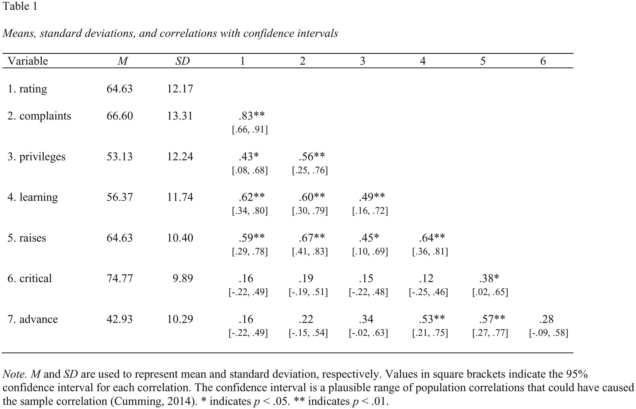
Screenshot of the Microsoft Word correlation table for the attitude data set.

It may be rare that one would want to create a correlation table using all of the columns in a data set. If we are interested in creating a correlation table based on a subset of the columns in the attitude data set, we can use the select command from the tidyverse package:

attitude_key_columns <- select(attitude, rating, complaints, learning, raises, advance)

This code creates a new data set, named attitude_key_columns, which is composed of only the “rating,” “complaints,” “learning,” “raises,” and “advance” columns from the attitude data set. We can then create a correlation table for just these columns using the following code:

table1 <- apa.cor.table(attitude_key_columns,

filename = “Table1.doc”,

table.number = 1)

Note that we continue to number tables sequentially in this Tutorial, using the table.number argument.

Multiple Regression Tables

A regression table can be constructed using the apa.reg.table command. The constructed table includes unstandardized regression coefficients (with confidence intervals), standardized regression coefficients (with confidence intervals), semipartial correlations squared (with confidence intervals), zero-order correlations, and overall fit of the model (indexed by R², with its confidence interval).

For the examples of regression and multiple regression tables in this section and the next, we use the album data set from Field, Miles, and Field (2012). This data set has 200 rows, each representing an album, and four columns: “adverts” (amount of money spent on advertising, in thousands of British pounds), “sales” (number of albums sold, in thousands), “airplay” (number of times songs from the album were played on radio in the week prior to the album’s release), and “attract” (attractiveness rating of the band members). To see the data associated with this data set, we can again use the View command; likewise, to see the variables’ details (i.e., the variable view in SPSS), we can use the glimpse command.

Although we use the apa.reg.table command in apaTables to create the regression tables in this section, we note that apaTables also has an apa.boot.reg.table command. The apa.boot.reg.table command generates tables in which confidence intervals are generated via bootstrapping using the boot package (Canty & Ripley, 2017). With the latter command, confidence intervals are adjusted for proportion-of-variance statistics (e.g., sr², R²) using Algina, Keselman, and Penfield’s (2007) procedure.

We begin by using the library command to open the package we will use to make the basic regression table:

library(apaTables)

Following is the code for creating a basic regression table for the album data set using sales as the criterion variable and adverts and airplay as the predictors:

basic_reg <- lm(sales ~ adverts + airplay, data = album)

table2 <- apa.reg.table(basic_reg,

filename = “Table2.doc”,

table.number = 2)

A screenshot of this Microsoft Word table is presented in Figure 5.

Fig. 5.

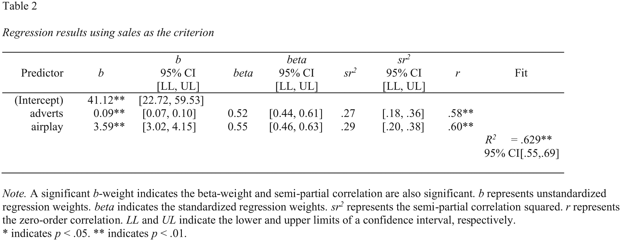
Screenshot of the Microsoft Word basic regression table for the album data set. CI = confidence interval.

Multiple Regression Tables With Blocks

In some cases, it can be useful for psychology researchers to compare the results of two regression models that have variables in common. This approach is often referred to as block-based regression. One common use of this approach is to “control” for certain variables (e.g., demographic or socioeconomic variables). In such a scenario, a researcher first conducts a regression with the control variables. This regression is referred to as Block 1. Next, the researcher conducts a second regression with the control variables and the substantive variables included. This second regression is referred to as Block 2. If Block 2 accounts for statistically significantly more variance in the criterion compared with Block 1, then the substantive variables are deemed to be meaningful predictors.

A second common use of block-based regression in psychology is to test for interactions between continuous variables. Consider a scenario in which a researcher uses two regressions to test for an interaction between two continuous variables. The Block 1 regression includes main effects for the two predictors of interest. The Block 2 regression includes the main effects of these two predictors of interest plus their product term. If Block 2 accounts for statistically significantly more variance in the criterion, above and beyond Block 1, an interaction is deemed to be present. Interactions can also be tested in a single regression; however, block-based regression is commonly used in psychology for this type of analysis. In the next example, we show how to use apaTables to create a table for a block-based regression examining whether advertisements and amount of airplay interact to predict sales in the album data set. Although this example uses only two blocks, note that any number of blocks can be used. If the predictors in any of the blocks are a product term, the zero-order correlation will be omitted from the output to prevent interpretation errors.

To create the multiblock regression table, we begin by opening the necessary package with the library command:

library(apaTables)

We then create the table with the following code. Do not forget to wrap the product term in the I() function to ensure correct results.

block1 <- lm(sales ~ adverts + airplay, data = album)

block2 <- lm(sales ~ adverts + airplay + I(adverts * airplay), data = album)

table3 <- apa.reg.table(block1, block2,

filename = “Table3.doc”,

table.number = 3)

A screenshot of this Microsoft Word table is presented in Figure 6.

Fig. 6.

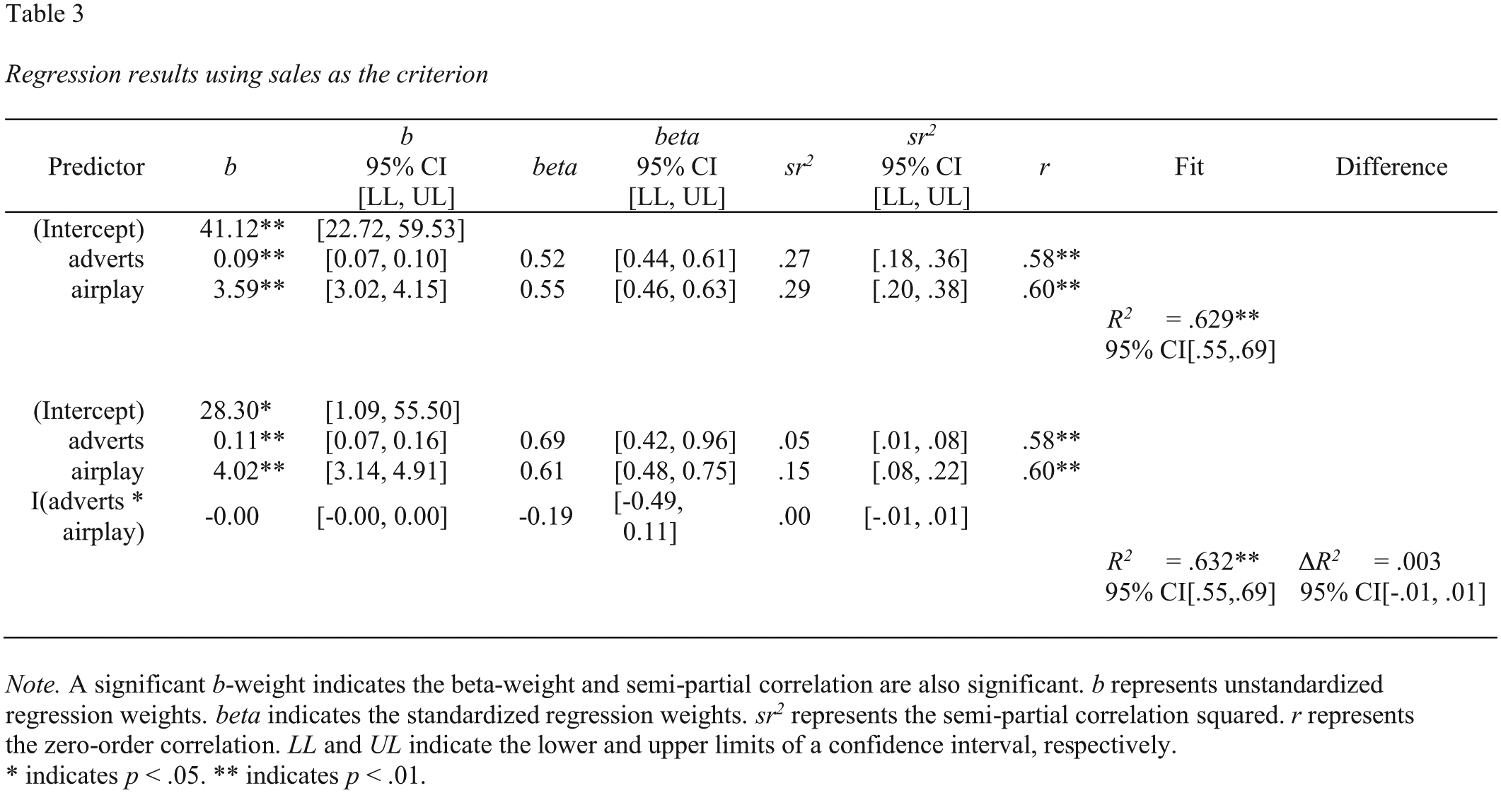
Screenshot of the Microsoft Word two-block multiple regression table for the album data set. CI = confidence interval.

Independent-Groups ANOVA Tables

One-way ANOVA and d-value tables

There are three commands in apaTables that are helpful for one-way ANOVAs with predictor variables that are independent: apa.aov.table, apa.1way.table, and apa.d.table. All three are illustrated here. ANOVA values in apaTables are calculated using the car package (Fox & Weisberg, 2011).

We begin by opening the packages we will use:

library(apaTables)

library(tidyverse)

Before an ANOVA table is generated, an ANOVA must be conducted. For our example, we use the viagra data set from Field et al. (2012). This data set contains 15 rows (one for each participant) and a column for each of two variables: dose and libido. Dose is a categorical variable that was made into a factor using the as_factor command in tidyverse. The dose variable has three levels: Placebo, Low Dose, and High Dose. The outcome variable is libido. The viagra data set can be viewed using the following command: View(viagra). The variable’s details can be obtained with the glimpse command:

glimpse(viagra)

Observations: 15

Variables: 2

$ dose <fct> Placebo, Placebo,…

$ libido <int> 3, 2, 1, 1, 4, 5,…

An inspection of this output reveals that the dose variable is a factor (i.e., categorical variable), as indicated by the “< fct >” to the right of this column name. In order to provide the correct values from an ANOVA, the R software must be able to identify that a variable is categorical (i.e., a factor, in R terms). If categorical variables are not identified as factors, an analysis will be run, and no error messages will appear, but the values provided will be incorrect. When you are conducting an ANOVA on your own data set, you must convert all categorical predictors (i.e., independent variables) into factor variables in R. This can be done with the as_factor command in the tidyverse package.³ For example, if the dose variable in the viagra data set were not a factor, it could be converted into one using this code:

viagra$dose <- as_factor(viagra$dose)

Note, however, that this code does not actually need to be run for the present example, because dose is already a factor in the viagra data set.

There are different ways to conduct an ANOVA in R. For example, one option is to use the aov command. The other is to use the lm command. We use the lm command for our examples of one-way and multiway ANOVAs because it handles unequal cell sizes well, whereas the aov command does not.

When using the lm command to conduct an ANOVA in R, you must ensure that your independent variables are R factors (as we have just explained) and that contrasts are set correctly. The following code configures the contrasts so that the R results will match those of SPSS (which may or may not be desirable):

options(contrasts = c(“contr.helmert”, “contr.poly”))

The next step is to conduct the ANOVA:

lm_output <- lm(libido ~ dose, data = viagra)

Finally, the apa.aov.table command will create a one-way ANOVA table based on lm_output:

table4 <- apa.aov.table(lm_output,

filename = “Table4.doc”,

table.number = 4)

A screenshot of this Microsoft Word table is presented in Figure 7.

Fig. 7.

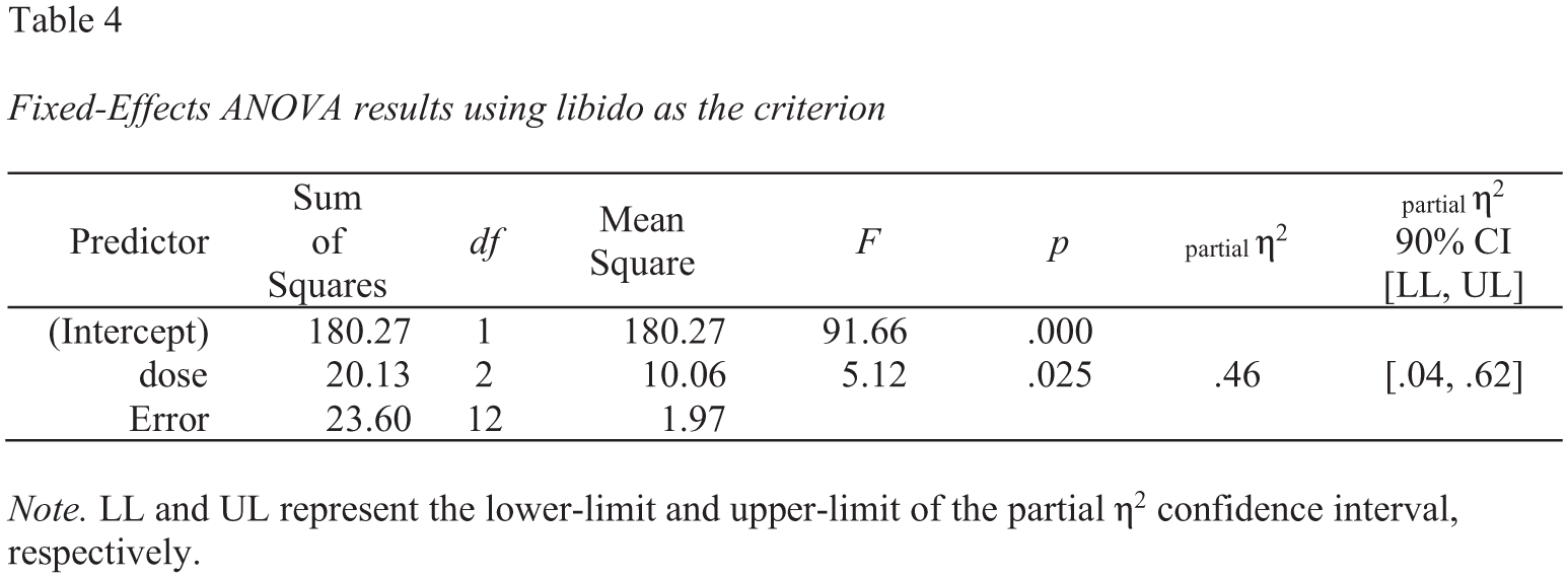
Screenshot of the Microsoft Word one-way analysis of variance (ANOVA) table for the viagra data set. CI = confidence interval.

To create a table with the mean and standard deviation for each cell in this analysis, we can use the apa.1way.table command. In this and later commands, iv and dv indicate the independent and dependent variables, respectively:

table5 <- apa.1way.table(iv = dose, dv = libido,

data = viagra,

filename = “Table5.doc”,

table.number = 5)

A screenshot of this Microsoft Word table is presented in Figure 8.

Fig. 8.

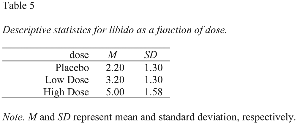
Screenshot of the Microsoft Word table for the descriptive statistics corresponding to the one-way analysis of variance in Figure 7.

The apa.d.table command creates a table containing d values, with confidence intervals (calculated via MBESS; Kelley, 2018), for each paired comparison. The layout of this table is similar to that of a correlation table, but in this case, the cells refer to paired comparisons rather than correlations. The d-value table for the present example can be created using the following code:

table6 <- apa.d.table(iv = dose, dv = libido,

data = viagra,

filename = “Table6.doc”,

table.number = 6)

A screenshot of this Microsoft Word table is presented in Figure 9.

Fig. 9.

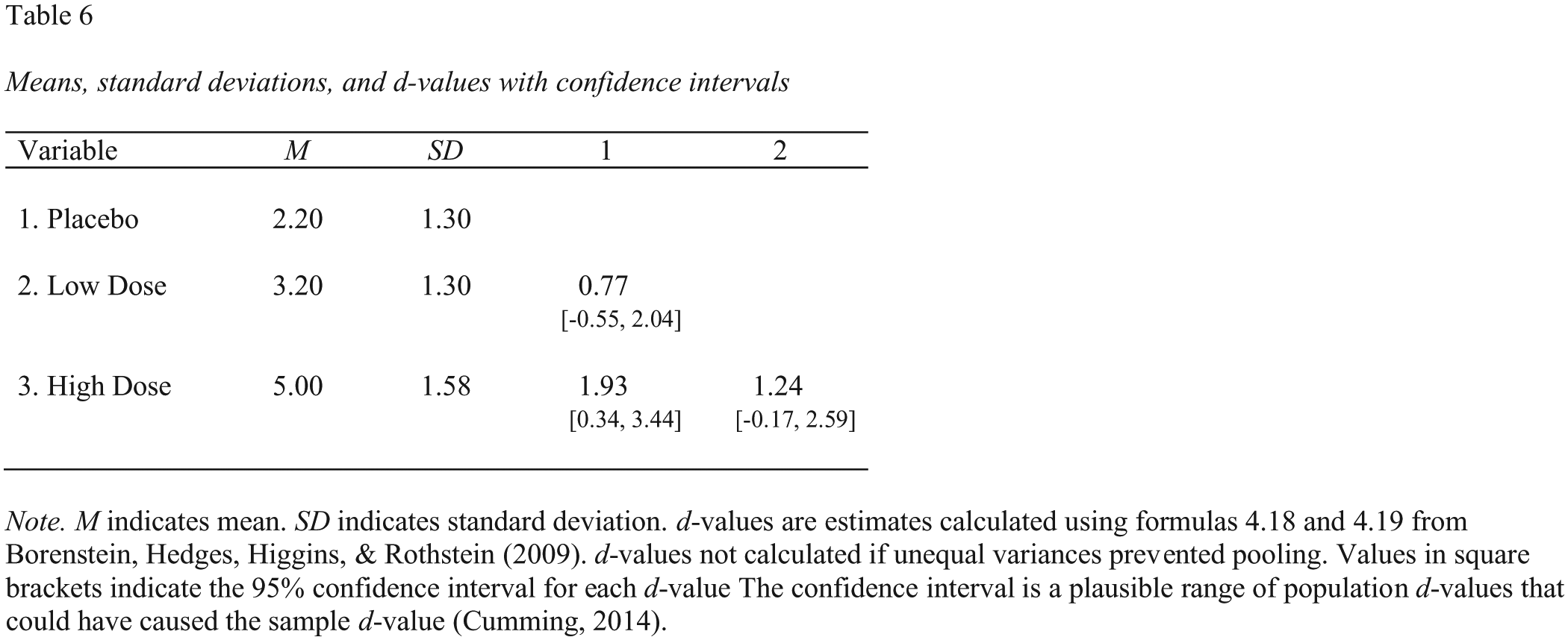
Screenshot of the Microsoft Word table for the descriptive statistics and paired-comparison d values (with 95% confidence intervals) corresponding to the one-way analysis of variance in Figure 7.

N-way independent-groups ANOVA tables: two-way example

The apa.aov.table command in apaTables handles all N-way ANOVA designs in which the predictors are categorical independent variables. Analyses with repeated measures are handled by apa.ezANOVA.table, which we discuss in the next section.

Again, we begin by opening the packages we will use in this section with the library command:

library(apaTables)

library(tidyverse)

The following two-way ANOVA example is based on the goggles data set from Field et al. (2012). The data set contains 48 rows and three variables. The variables are gender (gender of the participant), alcohol (amount of alcohol consumed), and attractiveness (perceived attractiveness of a target). We will conduct a 2 (gender: female, male) × 3 (alcohol: none, 2 pints, 4 pints) ANOVA in which attractiveness is the dependent variable.

As before, because we are conducting an ANOVA in R using the lm command, we must ensure that our independent variables are R factors and that contrasts are set correctly.

First, we want to check that both gender and alcohol are correctly coded factors, so we use the glimpse command:

glimpse(goggles)

Observations: 48

Variables: 4

$ participant <fct> 1, 2, 3, 4, 5,…

$ gender <fct> Female, Female…

$ alcohol <fct> None, None, No…

$ attractiveness <int> 65, 70, 60, 60…

The “<fct>” designation to the right of each column name indicates that these variables are indeed factors. If they were not, they could be converted to factors using the same process described earlier, for the one-way ANOVA table.

Second, we set the contrasts to ensure that the R output will match that of SPSS (which may or may not be desirable):

options(contrasts = c(“contr.helmert”, “contr.poly”))

Then, we conduct the ANOVA:

lm_output <- lm(attractiveness ~ gender * alcohol, data = goggles)

Next, we use the apa.aov.table command to create a two-way ANOVA table based on lm_output:

table7 <- apa.aov.table(lm_output,

filename = “Table7.doc”,

table.number = 7)

A screenshot of this Microsoft Word table is presented in Figure 10.

Fig. 10.

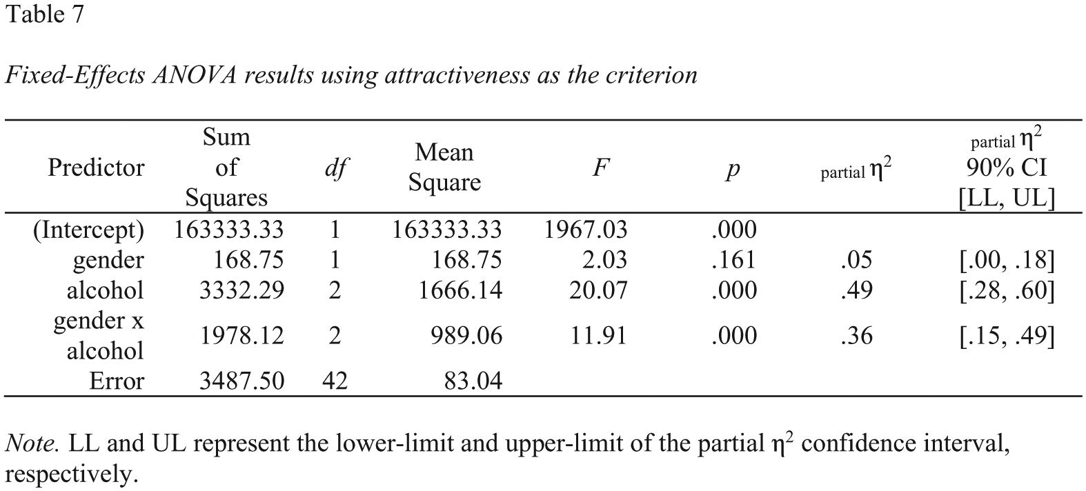
Screenshot of the Microsoft Word two-way analysis of variance (ANOVA) table for the goggles data set. CI = confidence interval.

We can also use the apa.2way.table command to create a table with the mean and standard deviation for each cell . Marginal means can also be requested (for details, see the help file in the R console: ?apa.2way.table), as in the following example:

table8 <- apa.2way.table (iv1 = gender,

iv2 = alcohol,

dv = attractiveness,

data = goggles,

filename = “Table8.doc”,

show.marginal.means = TRUE,

table.number = 8)

A screenshot of this Microsoft Word table is presented in Figure 11.

Fig. 11.

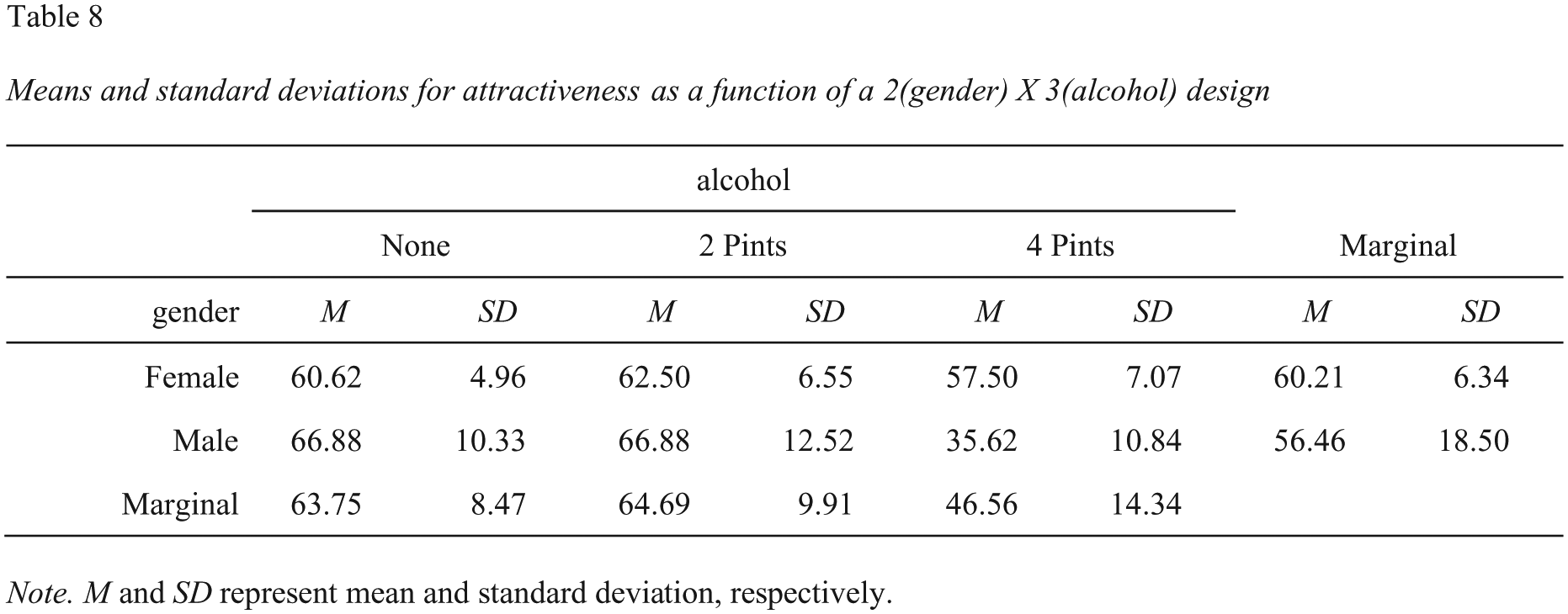
Screenshot of the Microsoft Word table for the descriptive statistics, with marginal means, corresponding to the two-way analysis of variance in Figure 10.

For higher-order ANOVA designs (i.e., three-way or higher), use the filter command from the tidyverse package to select the subset of rows of interest, and then use apa.2way.table to display cell statistics.

We can use the tidyverse package to conduct paired comparisons within each gender, again using apa.d.table. Prior to doing so, we use the filter command to generate separate data sets for male and female participants:

goggles_men <- filter(goggles, gender == “Male”)

goggles_women <- filter(goggles, gender == “Female”)

table9 <- apa.d.table(iv = alcohol,

dv = attractiveness,

data = goggles_men,

filename = “Table9.doc”,

table.number = 9)

table10 <- apa.d.table(iv = alcohol,

dv = attractiveness,

data = goggles_women,

filename = “Table10.doc”,

table.number = 10)

A screenshot of these Microsoft Word tables is presented in Figure 12.

Fig. 12.

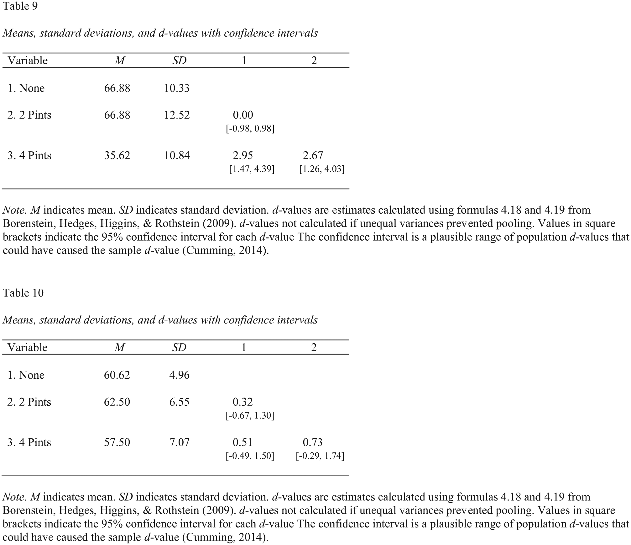
Screenshot of the Microsoft Word subgroup tables for the descriptive statistics and paired-comparison d values corresponding to the two-way analysis of variance in Figure 10. Table 9 shows the results for men, and Table 10 shows the results for women.

Repeated Measures ANOVA: ezANOVA Meet apaTables

The apaTables package also supports repeated measures ANOVA tables and mixed-design (combined repeated measures and between-subjects design ANOVA tables via ezANOVA output (Lawrence, 2016).

We begin by using the library command to open the packages we will use for our repeated measures ANOVA:

library(apaTables)

library(tidyverse)

library(ez)

In this example of an ANOVA with two repeated measures factors, we use the drink_attitude_wide data set from Field et al. (2012), which is built into apaTables. Note that we use the “wide” descriptor in the name of the data set (drink_attitude_wide) to remind ourselves that the data are in the wide format, in which one row contains all the data for one person. This format is the one used by SPSS to represent data. There are 20 participants in this data set, so there are 20 rows; in addition, there are 10 columns. The experiment has a 3 (drink: wine, beer, water) × 3 (imagery: positive, negative, neutral) design, and attitude is the dependent variable.

As before with ANOVA designs, we need to ensure that we represent the ANOVA predictors as categorical factors in R. However, because this is a repeated measures design, we also need a column that contains a participant identification number as a factor. Using the glimpse command, we obtain the following output:

glimpse(drink_attitude_wide)

Observations: 20

Variables: 10

$ participant <fct> P1, P2, P3, …

$ beer_positive <int> 1, 43, 15, 4…

$ beer_negative <int> 6, 30, 15, 3…

$ beer_neutral <int> 5, 8, 12, 19…

$ wine_positive <int> 38, 20, 20, …

$ wine_negative <int> -5, -12, -15…

$ wine_neutral <int> 4, 4, 6, 0, …

$ water_positive <int> 10, 9, 6, 20…

$ water_negative <int> -14, -10, -1…

$ water_neutral <int> -2, -13, 1, …

In this wide-format data set, the first column contains a code for each participant (P1, P2, etc.), and the “< fct >” designation to the right of the column name indicates that this variable is a factor. There are nine cells in our 3 (drink: wine, beer, water) × 3 (imagery: positive, negative, neutral) repeated measures design, and the data for these nine cells are contained in the remaining nine columns in the data set. Each of these nine columns contains attitude ratings for a single combination of the drink and imagery variables.

To run a repeated measures ANOVA with your own wide-format data set, you will need to ensure that the columns are named using the naming convention we describe next. Indeed, the naming convention for columns is critical to the workflow we describe.

In the wide format, each column name indicates the levels of the repeated measures factors that were combined to create it, separated by an underscore (_). Specifically, in the drink_attitude_wide data, the name for each column consists of the level of the drink variable, an underscore, and the level of the imagery variable. For example, the column called “beer_positive” represents the cell with a combination of the beer level of drink and the positive level of imagery. Each value in this column represents attitude for a participant in this cell. This naming convention, using the underscore, can be extended to any number of predictors.

Unfortunately, with a data set in this wide format, we do not a have a single column for each of the ANOVA factors (drink and imagery). We will need to create these columns prior to running the analysis. The lengthy process for converting the data to a format with a single column for drink and a single column for imagery is called converting the data to long format.

To convert the data to long format, we use the gather command from the tidyverse package:

drink_attitude_long <- gather (data = drink_attitude_wide,

key = cell, value = attitude,

beer_positive:water_neutral,

factor_key = TRUE)

This command creates a new data set in which there is a participant column, a cell column that indicates the cell an observation came from (e.g., beer_positive), and an attitude column that contains the attitude rating. Note that we use “beer_positive:water_neutral” to select all the columns in the data set between and including “beer_positive” and “water_neutral” (i.e., all nine columns). The columns must be in a block in the data set without other variables interspersed between them.

In this new long data set, each of the 20 participants has nine observations (i.e., nine cells), so there are 180 rows. Here are the first several rows:

head(drink_attitude_long)

# A tibble: 6 x 3

participant cell attitude

1 P1 beer_positive 1

2 P2 beer_positive 43

3 P3 beer_positive 15

4 P4 beer_positive 40

5 P5 beer_positive 8

6 P6 beer_positive 17

A problem, however, with this version of drink_attitude_long is that the levels of drink and imagery are combined into a single column called “cell.” That is, a cell contains the information in the form of, for example, “beer_positive” (i.e., the previous column names for the cells). To run the ANOVA, we need one column with the levels of drink and another column with the levels of imagery. Fortunately, because we previously used a naming convention in which an underscore separated the levels, the separate command in tidyverse easily creates those columns:

drink_attitude_long <- separate(data = drink_attitude_long,

col = cell,

into = c(“drink”, “imagery”),

sep = “_”, remove = TRUE)

This command creates the separate “drink” and “imagery” columns we need to run the analysis. However, by using the glimpse command, we can see that these newly created variables are not factors:

glimpse(drink_attitude_long)

Observations: 180

Variables: 4

$ participant <fct> P1, P2, P3, P4,…

$ drink <chr> “beer”, “beer”,…

$ imagery <chr> “positive”, “po…

$ attitude <int> 1, 43, 15, 40, …

We can convert the “drink” and “imagery” columns into factors with the as_factor command:

drink_attitude_long$drink <- as_factor(drink_attitude_long$ drink)

drink_attitude_long$imagery <- as_factor(drink_attitude_long$ imagery)

We can inspect and confirm the final long version of the data set with the glimpse command again:

glimpse(drink_attitude_long)

Observations: 180

Variables: 4

$ participant <fct> P1, P2, P3, P4,…

$ drink <fct> beer, beer, bee…

$ imagery <fct> positive, posit…

$ attitude <int> 1, 43, 15, 40, …

This output reveals the new appropriate data structure. There are now only four columns, and each row represents a single observation for a participant. As before, the first column is a factor column representing the participant variable. But each participant is represented nine times in this column now, because each participant has nine observations (i.e., one in each of the nine cells). Most important, we now have a single column indicating level of the drink variable, a single column indicating level of the imagery variable, and a column indicating the attitude rating.

We can see the first few rows of this data format using the following code:

head(drink_attitude_long)

# A tibble: 6 x 4

participant drink imagery attitude

1 P1 beer positive1

2 P2 beer positive43

3 P3 beer positive15

4 P4 beer positive40

5 P5 beer positive8

6 P6 beer positive17

Prior to conducting the analysis, we set the contrasts as per Field et al. (2012):

alcohol_vs_water <- c(1, 1, -2)

beer_vs_wine <- c(-1, 1, 0)

negative_vs_other <- c(1, -2, 1)

positive_vs_neutral <- c(-1, 0, 1)

contrasts(drink_attitude_long$drink) <- cbind(alcohol_vs_water, beer_vs_wine)

contrasts(drink_attitude_long$imagery) <- cbind(negative_vs_other, positive_vs_neutral)

Then, we use the ezANOVA command from the ez package to conduct the repeated measures ANOVA:

options(digits = 10)

drink_attitude_results <- ezANOVA(data = drink_attitude_long,

dv = .(attitude),

wid = .(participant),

within = .(drink, imagery),

type = 3, detailed = TRUE)

Note that the options command is needed before the ezANOVA command to ensure that the output has a sufficient number of digits (i.e., numbers after the decimal) for apaTables.

Next, we make the table based on the output:

table11 <- apa.ezANOVA.table (drink_attitude_results,

table.number = 11,

filename= “Table_11.doc”)

A screenshot of this Microsoft Word table is presented in Figure 13.

Fig. 13.

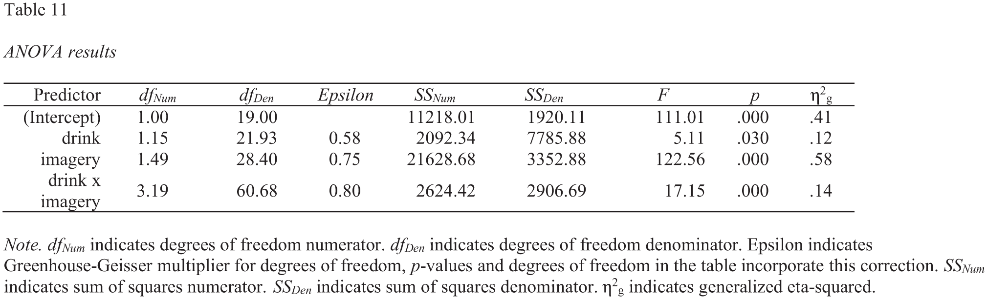
Screenshot of the Microsoft Word two-way repeated measures analysis of variance table for the drink_attitude_wide data set.

Instructions for creating APA tables for mixed (between-/within-subjects) ANOVA designs can be found in an online supplement at https://osf.io/jsvdz/.

A Few Technical Details

Feature requests and bug reports regarding apaTables can be filed at https://github.com/dstanley4/apaTables/issues. A key feature of open science is storing data in formats that are not proprietary. Consequently, all files created by apaTables are stored in the .rtf format despite the .doc extension. In the examples in this Tutorial, we ended all file names with .doc so that if you create these examples on your own macOS or Windows computer, the file names can be double-clicked and automatically opened by Microsoft Word (and automatically converted to Word format). However, researchers interested in using other word-processing software can simply end their file name with the .rtf extension.

We also add one caveat to our smartphone analogy. Smartphones automatically download app updates, but these processes must be done manually in R. Therefore, it is a good idea to use the install.packages command every few months to ensure that you have the latest versions of the packages you use.

Conclusion

The mounting recognition of the fallibility of the research process has generated calls to change how psychological research is conducted (Nosek et al., 2015). These calls have generally involved making a move toward open science, such that the original data and scripts can be used to verify the findings in an article (Nosek et al., 2015). Our software provides one answer to this call by automating the creation of APA-style tables in a way that increases efficiency, eliminates transcription errors, and increases the reproducibility of tables.

Supplemental Material

StanleyOpenPracticesDisclosure – Supplemental material for Reproducible Tables in Psychology Using the apaTables Package

Supplemental material, StanleyOpenPracticesDisclosure for Reproducible Tables in Psychology Using the apaTables Package by David J. Stanley and Jeffrey R. Spence in Advances in Methods and Practices in Psychological Science

Footnotes

Action Editor

Alex O. Holcombe served as action editor for this article.

Author Contributions

D. J. Stanley developed the R code, and D. J. Stanley and J. R. Spence wrote the manuscript.

Declaration of Conflicting Interests

The author(s) declared that there were no conflicts of interest with respect to the authorship or the publication of this article.

Open Practices

All materials have been made publicly available and can be accessed at https://osf.io/jsvdz/ and https://github.com/dstanley4/apaTables. The complete Open Practices Disclosure for this article can be found at http://journals.sagepub.com/doi/suppl/10.1177/2515245918773743. This article has received the badge for Open Materials. More information about the Open Practices badges can be found at .

Notes

References

Algina

Keselman

H. J.

Penfield

R. D.

(2007). Confidence intervals for an effect size measure in multiple linear regression. Education and Psychological Measurement, 67, 207–218.

American Psychological Association. (2010). Publication manual of the American Psychological Association (6th ed.). Washington, DC: Author.

American Statistical Association. (2016). American Statistical Association releases statement on statistical significance and p-values: Provides principles to improve the conduct and interpretation of quantitative science. Retrieved from https://www.amstat.org/newsroom/pressreleases/P-ValueStatement.pdf

Aust

Barth

(2018). papaja: Create APA manuscripts with R markdown (R package Version 0.1.0.9709) [Computer software]. Retrieved from https://github.com/crsh/papaja

Borenstein

Hedges

L. V.

Higgins

J. P. T.

Rothstein

H. R.

(2009). Introduction to meta-analysis. Chichester, England: Wiley.

Canty

Ripley

(2017). boot: Bootstrap R (S-Plus) Functions (R package Version 1.3-20) [Computer software]. Retrieved from https://cran.r-project.org/package=boot

Chatterjee

Price

(1977) Regression analysis by ex-ample. New York, NY: Wiley.

Cumming

(2014). The new statistics: why and how. Psychological Science, 25, 7-29.

Dahl

D. B.

(2016). xtable: Export tables to LaTeX or HTML (R package Version 1.8-2) [Computer software]. Retrieved from https://CRAN.R-project.org/package=xtable

10.

Field

Miles

Field

(2012). Discovering statistics using R. London, England: Sage.

11.

Fox

Weisberg

(2011). An R companion to applied regression (2nd ed.). Thousand Oaks, CA: Sage.

12.

Gordon

Gragg

Konings

(2018). htmlTable: Advanced tables for Markdown/HTML (R package Version 1.11.2) [Computer software]. Retrieved from https://CRAN.R-project.org/package=htmlTable

13.

Hajage

(2011). ascii: Export R objects to several markup languages (R package Version 2.1) [Computer software]. Retrieved from https://CRAN.R-project.org/package=ascii

14.

Hugh-Jones

(2018). huxtable: Easily create and style tables for LaTeX, HTML and other formats (R package Version 3.0.0) [Computer software]. Retrieved from https://CRAN.R-project.org/package=huxtable

15.

Ince

D. C.

Hatton

Graham-Cumming

(2012). The case for open computer programs. Nature, 482, 485–488.

16.

John

L. K.

Loewenstein

Prelec

(2012). Measuring the prevalence of questionable research practices with incentives for truth telling. Psychological Science, 23, 524–532.

17.

Kelley

(2018). MBESS: The MBESS R package (R package Version 4.4.3) [Computer software]. Retrieved from https://CRAN.R-project.org/package=MBESS

18.

Kim

A. Y.

(2018, January). Something old, something new, something borrowed, something blue. Presentation at Data Day Texas, Austin, TX

19.

Koenker

Zeileis

(2009). On reproducible econometric research. Journal of Applied Econometrics, 24, 833–847.

20.

Kuhn

(2018). CRAN task view: Reproducible research. Retrieved from https://cran.r-project.org/web/views/ReproducibleResearch.html

21.

Laine

Goodman

S. N.

Griswold

M. E.

Sox

H. C.

(2007). Reproducible research: Moving toward research the public can really trust. Annals of Internal Medicine, 146, 450–453.

22.

Lawrence

M. A.

(2016). ez: Easy analysis and visualization of factorial experiments (R package Version 4.4-0) [Computer software]. Retrieved from https://CRAN.R-project.org/package=ez

23.

Leland

, & Task Force on Statistical Inference, American Psychological Association, Science Directorate. (1999). Statistical methods in psychology journals: Guidelines and explanations. American Psychologist, 54, 594–604.

24.

Nosek

B. A.

Alter

Banks

G. C.

Borsboom

Bowman

S. D.

Breckler

S. J.

. . . Yarkoni

(2015). Promoting an open research culture. Science, 348, 1422–1425.

25.

Nuijten

M. B.

Hartgerink

C. H. J.

van Assen

M. A. L. M.

Epskamp

Wicherts

J. M.

(2016). The prevalence of statistical reporting errors in psychology (1985–2013). Behavior Research Methods, 48, 1205–1226.

26.

Open Science Collaboration. (2012). An open, large-scale, collaborative effort to estimate the reproducibility of psychological science. Perspectives on Psychological Science, 7, 657–660.

27.

Open Science Collaboration. (2015). Estimating the reproducibility of psychological science. Science, 349, Article aac4716. Retrieved from http://science.sciencemag.org/content/349/6251/aac4716/tab-pdf

28.

Pashler

Wagenmakers

E.-J.

(2012). Editors’ introduction to the special section on replicability in psychological science: A crisis of confidence? Perspectives on Psychological Science, 7, 528–530.

29.

Peng

R. D.

(2009). Reproducible research and biostatistics. Biostatistics, 10, 405–408.

30.

Peng

R. D.

(2011). Reproducible research in computational science. Science, 334, 1226–1227.

31.

Peng

R. D.

Dominici

Zeger

S. L.

(2006). Reproducible epidemiologic research. American Journal of Epidemiology, 163, 783–789.

32.

R Core Team. (2018). R: A language and environment for statistical computing. Retrieved from http://www.R-project.org/

33.

Retraction Watch. (2016, March 7). We’re using a common statistical test all wrong. Statisticians want to fix that. Retrieved from http://retractionwatch.com/2016/03/07/were-using-a-common-statistical-test-all-wrong-statisticians-want-to-fix-that/

34.

Revelle

(2017). psych: Procedures for personality and psychological research (R package Version 1.7.5) [Computer software]. Retrieved from https://CRAN.R-project.org/package=psych

35.

Stanley

D. J.

Spence

J. R.

(2014). Expectations for replications: Are yours realistic? Perspectives on Psychological Science, 9, 305–318.

36.

Wickham

(2017). tidyverse: Easily install and load the ‘Tidyverse’ (R package Version 1.2.1) [Computer software]. Retrieved from https://CRAN.R-project.org/package=tidyverse

37.

Wickham

(2018). Package ‘forcats’ (Version 0.3.0) [Computer software]. Retrieved from https://cran.r-project.org/web/packages/forcats/forcats.pdf

38.

Winerman

(2017). Trends report: Psychologists embrace open science. Monitor on Psychology. Retrieved from http://www.apa.org/monitor/2017/11/trends-open-science.aspx

Supplementary Material

Please find the following supplemental material available below.

For Open Access articles published under a Creative Commons License, all supplemental material carries the same license as the article it is associated with.

For non-Open Access articles published, all supplemental material carries a non-exclusive license, and permission requests for re-use of supplemental material or any part of supplemental material shall be sent directly to the copyright owner as specified in the copyright notice associated with the article.

0.00 MB

0.25 MB