Sage Journals: Discover world-class research

Abstract

Psychological science relies on behavioral measures to assess cognitive processing; however, the field has not yet developed a tradition of routinely examining the reliability of these behavioral measures. Reliable measures are essential to draw robust inferences from statistical analyses, and subpar reliability has severe implications for measures’ validity and interpretation. Without examining and reporting the reliability of measurements used in an analysis, it is nearly impossible to ascertain whether results are robust or have arisen largely from measurement error. In this article, we propose that researchers adopt a standard practice of estimating and reporting the reliability of behavioral assessments of cognitive processing. We illustrate the need for this practice using an example from experimental psychopathology, the dot-probe task, although we argue that reporting reliability is relevant across fields (e.g., social cognition and cognitive psychology). We explore several implications of low measurement reliability and the detrimental impact that failure to assess measurement reliability has on interpretability and comparison of results and therefore research quality. We argue that researchers in the field of cognition need to report measurement reliability as routine practice so that more reliable assessment tools can be developed. To provide some guidance on estimating and reporting reliability, we describe the use of bootstrapped split-half estimation and intraclass correlation coefficients to estimate internal consistency and test-retest reliability, respectively. For future researchers to build upon current results, it is imperative that all researchers provide psychometric information sufficient for estimating the accuracy of inferences and informing further development of cognitive-behavioral assessments.

Keywords

reliability estimating and reporting cognitive-behavioral tasks psychometrics open materials

In essence, it is as if I-P [information-processing] researchers have been granted psychometric free rein that would probably never be extended to researchers using other measures, such as questionnaires.

—Vasey, Dalgleish, and Silverman (2003, p. 84)

The central argument of this article is that psychological science stands to benefit greatly from adopting a standard practice of estimating and reporting the reliability of behavioral assessments. Behavioral assessments are commonly used in psychological science to examine cognitive processing, yet they rarely receive sufficient psychometric scrutiny. Here, we outline how reporting basic psychometrics will improve current research practices in psychological science. We use an example from experimental psychopathology showing that early adoption of such a practice would have avoided years of research using measures unsuited to individual differences research. More generally, our recommendations apply to any approach that relies on behavioral measures of cognitive functions, which we refer to as cognitive-behavioral measures. We echo the concern Vasey et al. (2003) expressed 16 years ago in the passage we quoted to open this article. Our impression is that although pockets of information-processing researchers have begun to appreciate the importance of measure reliability, little has changed in practice. We hope that this article helps to spark the small changes required to achieve a conceivably significant improvement in the quality and practice of research in experimental psychopathology, as well as psychological science more generally.

All measures, and therefore all analyses, are “contaminated” by measurement error. Reliability estimates provide researchers with an indication of the degree of contamination, enabling better judgments about the implications of their analyses. Various authors have stressed the importance of measurement reliability. For example, Wilkinson and the Task Force on Statistical Inference (1999) wrote that “interpreting the size of observed effects requires an assessment of the reliability of the scores” (p. 596), and LeBel and Paunonen (2011) recommended that researchers “calibrate their confidence in their experimental results as a function of the amount of random measurement error contaminating the scores of the dependent variable” (p. 578; also see Cooper, Gonthier, Barch, & Braver, 2017; Hedge, Powell, & Sumner, 2018). Psychometric consideration is usually afforded to self-report measures, but we argue that such consideration is equally important for cognitive-behavioral measures.

Reliability is not an inherent property of a task. Therefore, neither the term reliability nor obtained estimates of reliability should be ascribed to the task itself; reliability refers to the measurement obtained and not to the task used to obtain it. Many authors have made this same point (for a few examples, see Appelbaum et al., 2018; Cooper et al., 2017; Hedge et al., 2018; LeBel & Paunonen, 2011; and Wilkinson & Task Force on Statistical Inference, 1999). Nonetheless, it is warranted to emphasize that reliability is estimated from the scores obtained with a particular task performed by a particular sample under specific circumstances (we use measure and measurement throughout this article to refer to the measurements obtained, and not the task used). One cannot infer that a reliability estimate obtained for a certain measure in one sample, or reported in a test manual, will generalize to other study samples performing the same task. (Assuming that one’s measure is reliable, solely on the basis of other researchers’ reliability estimates, has been described as “reliability induction”—Vacha-Haase, Henson, & Caruso, 2002). Thus, researchers cannot assume a level of reliability in their measures without examining the psychometric properties of those measures in their particular study sample. It is, therefore, not surprising that psychological researchers are expected to report reliability and validity evidence for self-report questionnaires (e.g., the American Psychological Association’s reporting guidelines—Appelbaum et al., 2018). However, recent evidence has demonstrated that evidence for scale validity and reliability is severely underreported (Flake, Pek, & Hehman, 2017), and that crucial validity issues—such as lack of measurement invariance—remain hidden because of this underreporting (Hussey & Hughes, 2018).

This article is specifically concerned with the psychometrics of cognitive-behavioral tasks. Unfortunately, appraising the psychometrics of the measures obtained with these tasks is the exception rather than the rule (Gawronski, Deutsch, & Banse, 2011; Vasey et al., 2003). One reason for this may be that these tasks—unlike standardized questionnaires, for example—are often adapted to the research question, such as by modifying the task stimuli. In the absence of a standard practice of reporting the psychometrics of cognitive-behavioral measures, it is (a) difficult to determine how common or widespread it is for them to have reliability problems; (b) nearly impossible to assess the validity of previous research using these measures; (c) challenging to verify if changes to them result in improved reliability or validity; and (d) difficult, if not impossible, to compare effect sizes between studies. Cumulative science rests on the foundations of measurements, and building a sound research base is possible only when researchers report measurement psychometrics for all studies. Therefore, we recommend that psychological researchers estimate and report measurement reliability as standard practice, whether their work uses questionnaires or cognitive-behavioral measures.

This article is split into two parts. In the first part, we discuss the implications of measurement reliability for results, and the fact that these implications are often hidden because of lack of reporting. We then discuss an example from our field of experimental psychopathology to highlight some of these issues more concretely. In the second part of this article, we provide practical guidance on implementing the routine reporting of internal consistency and test-retest reliability estimates. We also provide example code to obtain reliability estimates, using simple commands in the R environment¹ to analyze publicly available Stroop-task data (Hedge et al., 2018). Finally, we make suggestions for the transparent and complete reporting of reliability estimates.

Disclosures

The code used to generate the reliability estimates in this article is available at the Open Science Framework (OSF), at https://osf.io/9jp65/. The files at OSF also include a copy of the data provided by Hedge et al. (2018), the submitted version of this manuscript, and the R Markdown script used to generate it.

On the Importance of Measurement Reliability

In this section, we highlight two areas of research where reliability plays an important role: statistical power and comparisons of results. For the impact of reliability in both areas to be evaluated, a standard practice of reporting reliability estimates will be necessary.

Reliability and statistical power

Low statistical power is an ongoing problem in psychological science (e.g., Button, Lewis, Penton-Voak, & Munafò, 2013; Morey & Lakens, 2016). Statistical power is the probability of observing a statistically significant effect for a given alpha (typically .05), sample size, and (nonzero) population effect. An often-overlooked fact is that low power, in addition to resulting in a low probability of observing effects that do exist (i.e., a high probability of committing Type II errors), increases the likelihood that any observed statistically significant effects are false positives (Ioannidis, 2005; Ioannidis, Tarone, & McLaughlin, 2011). Overlooking the influence of measurement reliability on statistical power means that its possible influence on the precision of statistical tests is unknown. In this section, we explore the relationship between statistical power and reliability in the case of both group-differences and individual differences designs.

Power, reliability, and group differences

Reliability has an indirect functional relationship with statistical power, which we illustrate here using a simple group-differences test as an example. Statistical power is dependent on both group sizes and measurement variance: Lower variance yields higher statistical power. As defined by classical test theory, observed-score variance (X), or total variance, is the sum of true-score variance (T) and error variance (E; i.e., X = T + E). Power depends on the total variance, that is, the sum of true-score and error variance. Measurement reliability (R), on the other hand, is defined as the proportion of variance attributed to true-score relative to total variance (i.e., R = T/T + E). As Zimmerman and Zumbo (2015) demonstrated mathematically, the relationship between reliability and power can be observed by holding either true-score variance or error variance constant and leaving the other to vary. By adding true-score or error variance, one increases the total variance and can observe the ensuing relationship between reliability and power. Briefly, when true variance is fixed, increases in error variance result in decreases in reliability and decreases in statistical power. In contrast, fixing error variance and increasing true variance leads to increases in reliability, but with decreases in power.

Visualizing these relationships can be helpful for understanding the conceptual difference between reductions in power due to increased error variance and reductions in power due to increased true variance. Figure 1 presents a visual representation of the relationship between variance and reliability. In the left graph, true-score variance is constant, whereas in the right graph, error variance is constant. Note the resulting reliability (T/T + E) on the y-axes and consider the impact of increasing total variance in both graphs. As total variance increases (i.e., as the width of the error bars increases), the observed effect size, $\frac{mean - 0}{\sqrt{total variance}}$ , is reduced. Consequently, statistical power is also reduced proportionally to the increase in total variance. However, the relationship between reliability and statistical power is different between the two scenarios. In the left graph, despite there being a consistent true difference from zero, increases in measurement error obscure the effect: As error increases, the true effect is hidden by error. In the right graph, on the other hand, the true effect size decreases as true variance increases, so statistical power is reduced (i.e., one needs larger samples to reliably detect an effect that shows a larger true variance). So, although reliability does not have a direct relationship to statistical power, it does offer useful information to aid the interpretations of results. For instance, it allows one to better gauge whether an observed small effect (in a study with low power) is due to measurement error obscuring the effect or is likely a genuinely small effect.

Fig. 1.

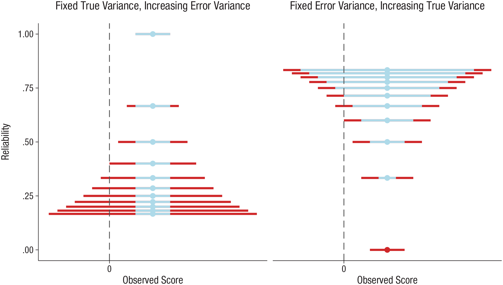
The relationship between reliability and variance. Both graphs show comparisons between observed measurement distributions and a reference value of zero (the dashed vertical lines). The blue sections of the distributions represent the true-score variance (T), and the red sections represent the error variance (E); the total width indicates the total variance. The corresponding reliability estimates (T/T + E) are indicated on the y-axis. The left-hand graph illustrates the decrease in reliability and increase in total variance that occurs when error variance increases while true-score variance remains constant. Thus, power changes despite no change in the true effect. The right-hand graph illustrates the decrease in both reliability and total variance that occurs when true-score variance decreases while error variance remains constant. Thus, power is reduced when the size of the true effect is smaller.

Power, reliability, and correlation: correcting for reliability

The reliability of measures constrains the maximum observable correlation between two measures: One cannot observe an association between two variables that is larger than the average reliability of those variables. Thus, greater measurement error and reduced between-subjects variance reduces the ability to observe associations between cognitive processes (also see Rouder, Kumar, & Haaf, 2019). To estimate this impact, one can begin with Spearman’s (1904) formula (also known as the attenuation-correction formula) to correct for the influence of measurement error on correlational analysis:

\begin{array}{r} r_{true} = \frac{r_{observed}}{\sqrt{r_{x x} \times r_{y y}}} \end{array}

(1)

Reliability estimates are estimates of variables’ autocorrelations (i.e., r_xx and r_yy in Equation 1). In other words, Spearman’s formula says that the true correlation between the true scores of x and y is the observed correlation divided by the square root of the product of the autocorrelations for both measurements. The formula can be rearranged to the following:

\begin{array}{r} r_{observed} = r_{true} \sqrt{R (x) \times R (y)} \end{array}

(2)

Using the rearranged formula, one can calculate the expected observed correlation and hence the power to detect a correlation in a study that has been powered at 80% to detect a correlation of at least the size of the expected true correlation. For example, if the expected true correlation between two measures in a study is .50 and both measures have reliability of .90, the observable correlation drops to .45:

\begin{array}{r} r_{observed} = . 50 \sqrt{. 90 \times . 90} = . 45 \end{array}

(3)

If 28 subjects were recruited to achieve 80% power to detect a correlation of .50, the fact that each measure had a reliability coefficient of .90 means that the study’s actual power (to detect an r of .45) was 69.5% rather than 80%. To regain the desired 80% power, a sample of 36 subjects would be required. Given that .90 reliability for both measures would be considered quite excellent, this example shows the large impact that measurement reliability has on power. Further illustrating this point, Figure 2 presents the required sample size to achieve 80% statistical power to detect true correlations of .3, .5, and .7, across a range of reliability estimates for both measures. Note that Hedge et al. (2018, Table 5) presented a similar argument.

Fig. 2.

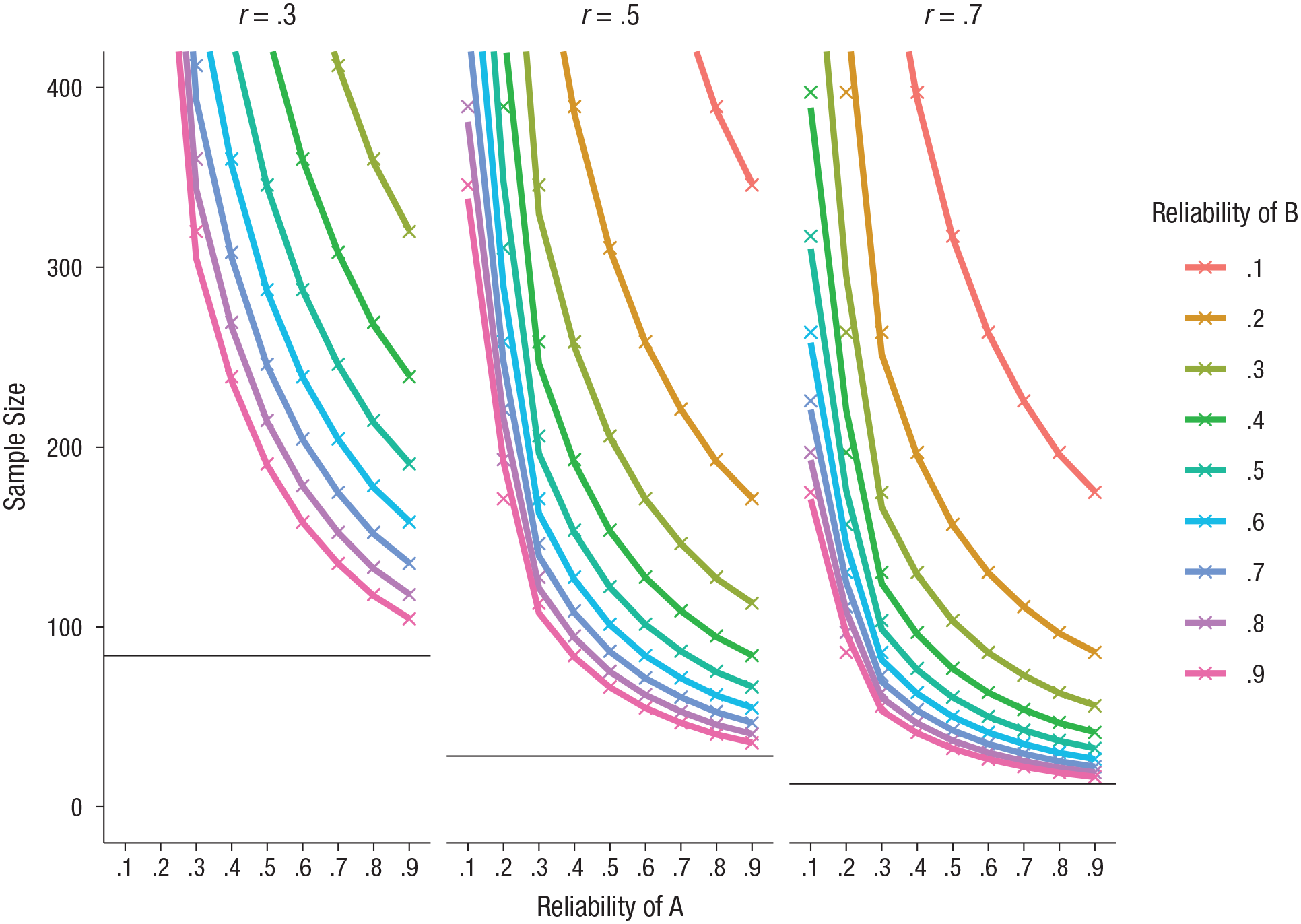
Required sample size for 80% power to detect true correlations of .3, .5, and .7 between measures A and B after correction for their reliability. The horizontal lines indicate the sample size required assuming perfect reliability of the two measures. For readers who may have a gray-scale version of this figure, the left-to-right order of the lines in the graphs matches the bottom-to-top order in the color key.

Readers who are interested in applying multilevel modeling to correct for the influence of measurement error may want to consult two recent publications exploring the use of hierarchical models to account for one source of error variance, namely, trial-level variation (Rouder & Haaf, 2018b; Rouder et al., 2019). None of the models tested by Rouder et al. (2019) performed well enough to accurately recover the simulated effect size. But these trial-level hierarchical models did outperform Spearman’s attenuation-correction formula (which can be unstable). The authors argued that error variance (measurement noise) may render the true-variance relationship between measures unrecoverable, and render it nearly impossible to answer questions about individual differences for certain measures. Yet hierarchical models are likely the best available tool to account for error. Hierarchical modeling including trial-level variation could routinely account for error in measures. However, in our experience, it is not yet standard for hierarchical models to be used to analyze data from behavioral tasks. We hope that the use of these models will become standard in the upcoming years. To help bridge this gap, we advocate efforts to promote a greater, more widespread understanding of the importance of the psychometrics of behavioral measurements and a greater focus on a standard practice of reporting estimates of their internal consistency and test-retest reliability.

Reliability and comparability

Cooper et al. (2017) illustrated two potential pitfalls when comparing effect sizes without considering reliability, using data derived from the AX-CPT, a variant of the computerized continuous performance task, as an example. To illustrate a potential pitfall when comparing correlations between samples taken from different populations, they used AX-CPT data, including reliabilities, originally reported by Strauss et al. (2014). Cooper et al. noted that the observed correlations between AX-CPT performance and another task measure (performance on the relational and item-specific encoding task) were greater in the schizophrenia sample than in the control sample. Also, the AX-CPT measure had greater variance, and greater test-retest reliability across all trial types, in the schizophrenia sample compared with the control sample. Therefore, it cannot be ruled out that the differences between the samples in the correlation between performance on the two tasks was the result of differences in variance and reliability between the samples.

Cooper et al. (2017) next illustrated a potential pitfall when comparing findings of largely identical studies, which one might expect to have produced the same results: Differences in psychometric properties lead to incomparable effect sizes. For this demonstration, they used data from two studies (Gonthier, Macnamara, Chow, Conway, & Braver, 2016; Richmond, Redick, & Braver, 2016) that recruited separate samples from the same population to examine the relationship between AX-CPT performance and a measure of working memory capacity. Although both studies found a correlation between performance on one AX-CPT trial type and working memory capacity, only one of the studies found a correlation between performance on two other AX-CPT trial types and working memory capacity. Reliability of the measures also differed between the studies. Therefore, it is unclear whether the difference in correlations reflects a genuine difference in associations or is a by-product of psychometric differences. Taking a step further, other researchers have proposed that effect-size estimates should be corrected for measurement error by default, as arguably psychological research is typically concerned with the relationships between actual traits or constructs, rather than between measures of traits or constructs (Schmidt & Hunter, 1996). Correcting for error would enable direct comparisons between the effect sizes Cooper et al. reported, for example. Thus, adopting a standard practice of reporting reliability would allow for better generalizability of effect-size estimates as well as more accurate comparisons of effect sizes (including aggregation of effect sizes, as in meta-analyses).

An example from the field of experimental psychopathology: the dot-probe task

To build on the previous sections, we discuss an example from experimental psychopathology relating to selective attentional processing of emotional information (for reviews of this field, see, e.g., Cisler & Koster, 2010; Gotlib & Joormann, 2010; Yiend, 2010). We focus on a task frequently used to assess (and often, attempt to modify) selective attentional bias: the emotional dot-probe task (C. MacLeod, Mathews, & Tata, 1986). In a typical dot-probe task, two stimuli are presented simultaneously for a set presentation duration (e.g., 500 ms). Usually, one of the stimuli is emotional (e.g., threat related), and the other is neutral. Immediately after the stimuli disappear, a probe is presented, and subjects press a key to report the identity of the probe (e.g., whether it is the letter E or F). The outcome measure indexes attentional bias, calculated by subtracting the average response time (RT) for trials in which the probe appeared in the location of the emotional stimulus from the average RT for trials in which the probe appeared in the location of the neutral stimulus. Dot-probe studies have used many variations of the task, differing in the number of trials, the stimulus presentation duration, the stimulus sets, the type of stimuli used (e.g., words or images), the type of probes (and how easily they can be perceived), and even whether the task is to identify the probe or just the location of the probe.

The use of the dot-probe methodology has grown considerably over the past decade (Kruijt, Field, & Fox, 2016, Fig. S1), and the number of published studies now likely numbers in the thousands. Unfortunately, in a recent study, Rodebaugh et al. (2016) were able to identify only 13 studies for which the reliability of the dot-probe task was reported. This growth in use of the task occurred despite two early publications that highlighted its reliability problems (Schmukle, 2005; Staugaard, 2009). When reliability estimates for the dot-probe task are reported, they tend to be unacceptably low (as low as –.12 in Waechter, Nelson, Wright, Hyatt, & Oakman, 2014). It is important to note that the reported estimates range widely (e.g., r = .45 in Bar-Haim et al., 2010; r = −.23 to .70 in Enock, Hofmann, & McNally, 2014; r = .15 to .59 in Waechter & Stolz, 2015). Since 2014, there has been growing concern about the reliability of the task, and several articles have directly examined its psychometric properties (H. M. Brown et al., 2014; Kappenman, Farrens, Luck, & Proudfit, 2014; Price et al., 2015; Sigurjónsdóttir, Sigurðardóttir, Björnsson, & Kristjánsson, 2015; Waechter et al., 2014; Waechter & Stolz, 2015). Alongside widespread calls to develop more reliable measures (e.g., C. MacLeod & Grafton, 2016; Price et al., 2015; Rodebaugh et al., 2016; Waechter & Stolz, 2015), various recommendations have been made to improve the stability and reliability of the dot-probe task (e.g., Price et al., 2015). Yet a recent study found that a number of these recommendations did not lead to consistent improvements in reliability, and no version of the task (or strategy for processing its data) was found to have adequate reliability (Jones, Christiansen, & Field, 2018).

Had the psychometric properties of dot-probe data been investigated early on—and had it already been known that individual differences studies using measures with high noise are doomed to fail (Rouder et al., 2019)—extensive resources might never have been invested in individual differences research using this task. Similarly, early psychometric examination might have led to a different understanding of the meaning of dot-probe-derived attentional-bias indices and to powerful theoretical insights regarding attentional bias, perhaps heavily altering the trajectory of the field. For example, Rodebaugh et al. (2016) recently compared the reliability of dot-probe bias indices calculated using traditional difference scores with the reliability of dot-probe indices treating attentional bias as a dynamic process. They found that difference scores yielded low reliability, whereas scores that treated attentional bias as a dynamic process led to much-improved reliability estimates. This puts doubt on the theoretical position that attentional bias is stable over time and raises serious questions about the typical use of the dot-probe measure and the decades of previous research using it—including the research in which many variants of the dot-probe task were intended to modify attentional bias. Rodebaugh et al. convincingly argued that, even aside from the fact that low reliability raises questions about the robustness of previous results, the lack of reporting reliability threatens theoretical understanding of attentional bias. Although it is a problem that the dot-probe task tends to yield unreliable data, the more pressing barrier is the consistent failure to estimate and report the psychometrics of behavioral measures in the first instance.

It is not our intention to unduly attack the dot-probe task. We use this task, as one of many potential examples, to demonstrate how taking “psychometric free reign” (Vasey et al., 2003, p. 84) with behavioral measures is detrimental to cumulative science. Evidence demonstrating the dangers of taking such liberties continues to mount; poor reliability is detrimental to making sound theoretical inferences (Rodebaugh et al., 2016), psychometric information is commonly underreported (Barry, Chaney, Piazza-Gardner, & Chavarria, 2014; Flake et al., 2017; Slaney, Tkatchouk, Gabriel, & Maraun, 2009), and this lack of reporting may hide serious validity issues (Hussey & Hughes, 2018). The purpose of this article is not to quash any discussion or research through a generalized argument that the measures in psychological research are not reliable, but rather to convince researchers that the field stands to benefit from improved standards for reporting psychometrics.

Questions of experimental differences and of individual differences

The distinction between experimental research (e.g., research on the effects of manipulations) and individual differences research (e.g., correlational research) is worth briefly discussing (e.g., Borsboom, Kievit, Cervone, & Hood, 2009; Cronbach, 1957, 1975). Experimental analyses benefit from precision (e.g., Luck, 2019), which is necessarily paired with low between-individuals variance (De Schryver, Hughes, Rosseel, & De Houwer, 2016), and this is perhaps reflected in a desire for groups that are as homogeneous as possible (Hedge et al., 2018). However, low variance may be due to lack of sensitivity in a measure, and low variance within a homogeneous group may result in difficulties rank-ordering the individuals within the group. Regardless of the cause of low between-individuals (true) variance, when it is paired with any amount of error variance, low reliability can easily result. Many tasks clearly display robust between-group or between-condition differences, but they also tend to have suboptimal reliability for individual differences research (Hedge et al., 2018). One such task is the Stroop (1935) task. It has been asserted that the Stroop effect can be considered universal (i.e., one can safely assume that everyone is subject to the Stroop effect; C. M. MacLeod, 1991; Rouder & Haaf, 2018a). Yet the task does not demonstrate sufficient reliability to be useful for investigating questions about individual differences (Hedge et al., 2018; Rouder et al., 2019).

Thus, robust experimental effects should not be interpreted as an indication of a measure’s high reliability or validity, nor do they provide sufficient information on the applicability of the measure for individual differences research (Cooper et al., 2017; Hedge et al., 2018). Unfortunately, it is common for tasks developed for experimental settings to be used in individual differences research with little attention paid to their psychometric properties. As Rouder et al. (2019) recently demonstrated, the use of tasks with low reliability in studies focusing on individual differences is doomed to fail. Regardless of the research question and the analytic method used, high measurement error will be detrimental to the analysis and the inferences that can be drawn from it (e.g., Kanyongo, Brook, Kyei-Blankson, & Gocmen, 2007).

Barriers to a standard practice of reporting reliability

We see two main barriers to implementing a standard practice of estimating and reporting the reliability of cognitive-behavioral tasks. First, it may not even be possible to estimate reliability for some measures. Perhaps the task or the data processing required is too complex, or perhaps another characteristic of the task, sample, context, or data collected leads to difficulties in estimating reliability. In cases such as these, the authors might consider stating that to their knowledge, there is no appropriate procedure to estimate the reliability of the measure. This would have the benefit of transparency. Further, a consideration of reliability in the absence of a reliability estimate would help in tempering interpretations of results, if only by preempting an implicit assumption that a measure is perfectly reliable and valid. Second, there is a lack of education and—in some instances—tools needed to implement a practice of estimating and reporting reliability for cognitive-behavioral measures. Psychometric training in core psychology courses is often limited to calculating Cronbach’s alpha for self-report data, but this statistic, and similar reliability estimates, may not apply to cognitive-behavioral measures. If a suitable procedure to estimate reliability does not exist or is inaccessible, then it would be foolhardy to expect researchers to report reliability as standard practice. A similar argument was made regarding the use of Bayesian statistics and sparked the development of JASP, a free, open-source software that is similar to SPSS but has the capacity to perform Bayesian analyses in an accessible way (Love et al., 2019; Marsman & Wagenmakers, 2017; Wagenmakers et al., 2018). It is important to ensure that the tools required to estimate reliability are readily available and easy to use. Therefore, the second part of this article forms a brief tutorial (with R code, examples, and recommendations) on estimating and reporting reliability.

A Brief Introduction to Estimating and Reporting Measurement Reliability

In this section, we outline approaches to estimating and reporting the reliability of one’s task measurements. Figure 3 presents our core recommendations for estimating internal consistency and test-retest reliability in flowchart form. Before presenting our recommendations in detail, we discuss some general considerations for estimating and reporting reliability.

Fig. 3.

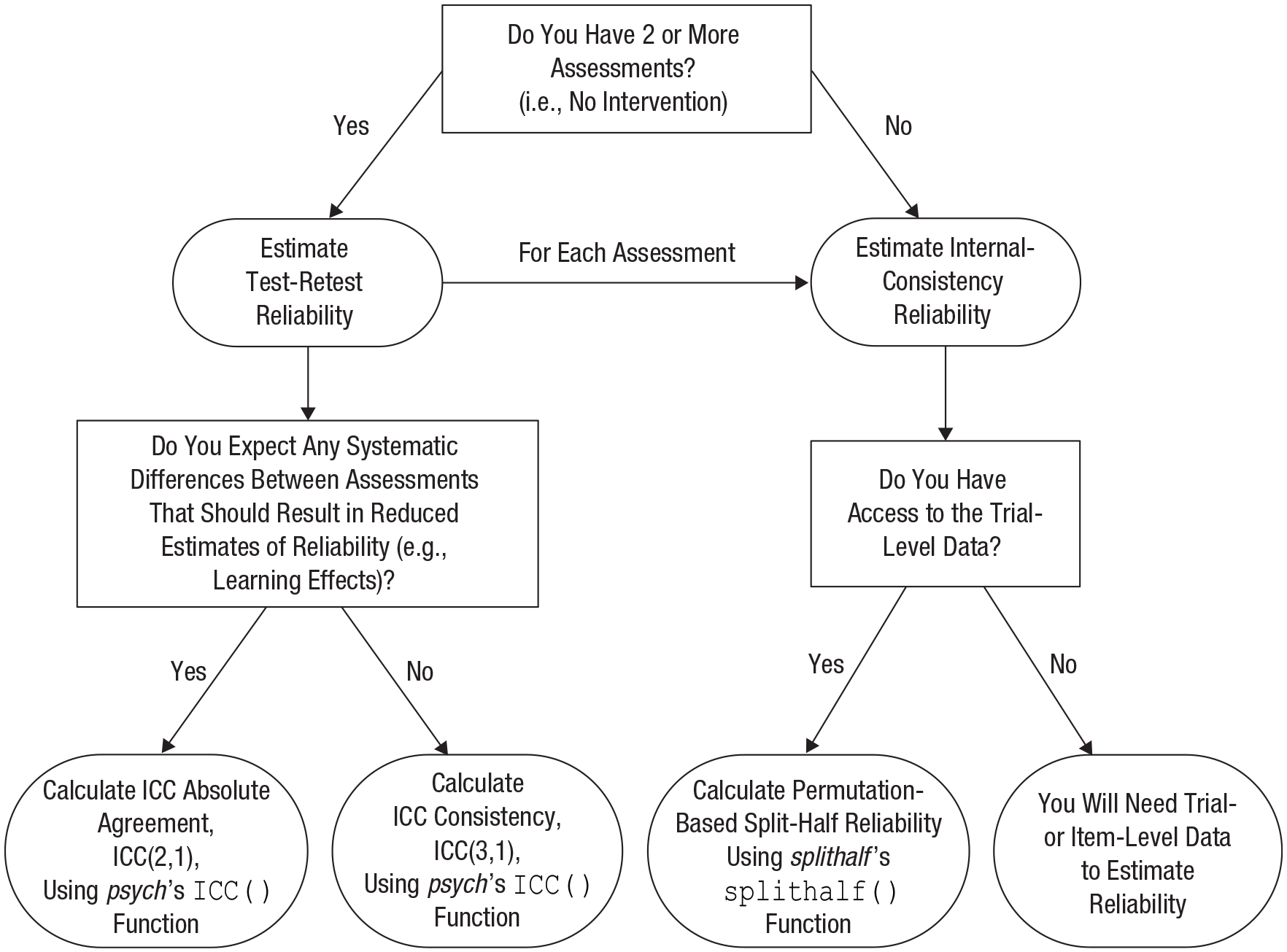
Flowchart of our core recommendations for reporting internal consistency and (if multiple measurements are available) test-retest reliability. ICC = intraclass correlation coefficient.

Matching reliability and outcome scores

Reliability estimates should be drawn from the same data as the outcome scores. For example, removal of outlier trials, subjects with high error rates, and so on, must be performed before reliability is estimated; indeed, data-reduction pipelines can have a surprising influence on reliability estimates. Similarly, if the outcome of interest entered into the analysis is a difference score, the reliability of the difference score (and not its components) should be determined. Likewise, if the sample has been divided into several groups, it follows that reliability should be estimated for each group. Reliability should be estimated for the actual outcome measures to be analyzed.

Reporting p values

We do not recommend that p values be reported alongside reliability estimates. In our view, it is often unclear what the p value adds or indicates in this context, and reporting this value opens the way for a potential misinterpretation that when a reliability estimate differs significantly from zero, one can be confident in the reliability of the measurement. On several occasions, we have observed statements describing a measurement’s reliability as being statistically significant even though the magnitude of the estimate is small (e.g., < .3); avoiding this misunderstanding by simply not reporting p values is preferable. Confidence intervals for reliability estimates, on the other hand, are informative, and we recommend reporting them.

Thresholds for reliability

We refrain from making specific recommendations for what should be considered “adequate” or “excellent” reliability. Reliability estimates are continuous, and using arbitrary thresholds may hinder their utility. Other researchers have suggested that .7 or .8 is a suitable threshold for reliability or have used labels for specific intervals (e.g., .50–.75 = “moderate” reliability, .75–.90 = “good” reliability, and > .90 = “excellent” reliability; Koo & Li, 2016). These labels should not be considered thresholds to pass, but rather should be considered another means to assess the validity of results based on these measures (Rodebaugh et al., 2016). A benefit of widespread reporting of reliability is that it would be possible to describe a task’s normative range of reliability estimates generated across samples, conditions, and task versions. Researchers would then have an almost metapsychometric reference point to compare with their estimates. Such comparisons are likely to be more useful than merely claiming that one’s measure has achieved “adequate” reliability.

Negative reliability estimates

It is possible for reliability estimates to be negative. At first sight, such a finding might seem to indicate that those individuals who scored highest on the first half of the task, scored lowest on the second, and vice versa (a conclusion that is mind-boggling in many contexts). However, negative reliability estimates can arise spuriously for at least two reasons. The first is that the data may violate the assumption of equal covariances among half-tests (Cronbach & Hartmann, 1954). The second cause of spurious negative reliability estimates is specific to difference scores (e.g., bias indices or gain scores). When the components of a difference score correlate highly, the variance of the difference score will approach zero. At zero variance, reliability is also zero, but because of imprecision in the estimate, the correlation between two assessments may appear to be negative. In such cases, it appears as if the data have an impossible covariance structure, with the total proportion of variance explained by the difference score plus its component scores surpassing the maximum value of 1 (all variance observed). In cases when an unlikely negative reliability estimate is obtained, we recommend reporting that negative estimate but interpreting it as equaling zero reliability (indeed, the value of 0 will typically be included in the estimate’s confidence interval).

Reporting the complete analysis

Even when ostensibly the same measure of reliability is used, different procedures for calculating the estimate may result in different estimates. For example, using a split-half approach, one could split trials into odd- and even-numbered trials or into the first half and second half of trials. Therefore, we recommend that authors report not only the reliability estimates themselves, but also the analysis procedures used to obtain those estimates. Such full reporting will facilitate transparency and reproducibility (providing analysis code would be ideal). Relevant details include if and how data were divided, the estimation method used, and the number of permutations or bootstraps, if applicable. Additionally, we recommend that confidence intervals be reported (e.g., Koo & Li, 2016) and note that reporting both corrected and uncorrected estimates (e.g., in the case of split-half reliability) can be useful to ease comparisons of estimates across studies.

Recommended methods for estimating reliability

For the following examples, we used Stroop-task data from Hedge et al. (2018). The data and code (see the R Markdown script) to re-create these analyses can be found on our project page at OSF (https://osf.io/9jp65/). Briefly, in Hedge et al.’s Stroop task, subjects made key-press responses to report the color of a word presented centrally on-screen. In congruent trials, the word’s meaning was the same as the font color. In incongruent trials, the word’s meaning was different from the font color. Subjects completed 240 trials of each trial type. For these examples, we focus on RT cost as the outcome measure; this cost is calculated by subtracting the mean RT in congruent trials from the mean RT in incongruent trials. Subjects completed the Stroop task twice, in sessions approximately 3 weeks apart. These separate sessions were useful for our purposes, because they allowed us to investigate both the internal consistency of each measurement separately and the test-retest reliability. Hedge et al. reported Stroop data from two separate studies; for simplicity, we have pooled these data. We followed their data-reduction procedures, and exact details can be found in the R Markdown version of our submitted manuscript at OSF (https://osf.io/9jp65/).

Internal consistency: permutation-based split-half correlations

Various statistical software programs offer the option to compute Cronbach’s alpha, yet many of these use an approach that is unlikely to be suitable for cognitive-behavioral tasks. The most commonly used approach amounts to averaging the correlations between each item’s score and the sum score of the remaining items. This approach assumes that Item 1, Item 2, Item 3, and so forth, have been identical for all subjects. It appears that to apply this approach to data from behavioral tasks, researchers often resort to creating bins of trials, each to be treated as an individual “item” or minitest. However, unless trial stimuli and conditions are presented in a fixed order, Cronbach’s alpha derived with this approach will not be a valid estimate of reliability. If one bins by trial number, then the stimuli within each bin will differ between subjects. If the same set of trials (same stimuli, etc.) have been presented to all subjects, with presentation order randomized for each subject, one could bin by stimulus (e.g., by specific pairing of word content and color in the Stroop example), yet each bin would contain trials from different stages of the task, which might reduce the obtained reliability estimate. We also note that although omega has been advocated as a robust estimate to replace alpha (Dunn, Baguley, & Brunsden, 2014; Peters, 2014; Sijtsma, 2009; Viladrich, Angulo-Brunet, & Doval, 2017), the same assumption that each bin is identical across subjects applies. Thus, the most common approach to obtaining alpha and omega is unsuitable for most task designs, except when a fixed trial and stimulus order was used.

However, averaging the correlations between each item’s score and the sum score of the other items is only one way to estimate alpha, which is defined as the average of all possible correlations between subsets of items. It is also possible to calculate alpha as the average of a sufficiently large number of split-half reliability estimates (Spearman, 1910) when each split-half reliability is based on a different random division of the items. In the split-half method as it is commonly applied, the data for a measure are split into two halves, typically into either the first and second half or the odd- and even-numbered items or trials. The Pearson correlation between these halves is then calculated as an estimate of the measure’s internal reliability. The Spearman-Brown (prophecy) formula (W. Brown, 1910; Spearman, 1910) is often subsequently applied to this estimation. This correction accounts for the underestimation resulting from splitting the number of observations in half to enable calculating a correlation. The Spearman-Brown corrected estimate is calculated as follows:

\begin{array}{r} r_{s} = \frac{2 r}{1 + r} \end{array}

(4)

When applied to tasks, standard split-half reliability estimates tend to be unstable. For example, reliability estimates obtained from splitting the data into odd- and even-numbered trials have the potential to vary greatly depending on which trials happened to be odd and even (Enock, Robinaugh, Reese, & McNally, 2012). Therefore, Enock et al. advocated estimating measurement reliability with a permutation approach, in which the data are repeatedly randomly split into two halves and the reliability estimate is calculated for each split (also see Cooper et al., 2017; J. W. MacLeod et al., 2010). The estimates are then averaged to provide a more stable estimate of reliability. It is important to note that Cronbach’s alpha can be defined as the average of all possible split-half reliabilities (Cronbach, 1951). Permutation-based split-half reliability, therefore, approximates Cronbach’s alpha, while avoiding the concerns we have discussed regarding estimating the internal consistency of cognitive-behavioral data. We recommend that researchers estimate and report permutation-based split-half reliabilities for their measures as estimates of internal-consistency reliability.

The R package splithalf (Parsons, 2019b) was developed to enable researchers with minimal programming experience to apply this method to (trial-level) task data with relative ease. Full documentation of the package, with examples, can be found online (Parsons, 2019a). Note that the online documentation will be the most up-to-date; for the examples in this article, we used Version 0.5.3, and future package versions may use a format different from the one in this article.

The permutation split-half approach can be performed on Hedge et al.’s (2018) Stroop data using the following code:

require(splithalf)

splithalf(data = Hedge_raw,

outcome = “RT”,

score = “difference”,

permutations = 5000,

var.trialnum = “Trial”,

var.condition = “time”,

conditionlist = c(1, 2),

var.compare = “Condition”,

compare1 = “congruent”,

compare2 = “incongruent”,

var.participant = “ppid”,

var.RT = “Reactiontime” )

The first line of code loads the splithalf package. The command splithalf() calls the function, and contained within the parentheses are the function parameters. This line specifies that the data to be processed are contained within the object Hedge_raw. The outcome of interest is the RT cost, which is calculated as the difference between the mean RT in congruent trials and the mean RT in incongruent trials. Thus, the outcome and score parameters are specified as RT and difference, respectively. Subsequent lines specify congruent and incongruent as the trial types between which the difference score is calculated. The parameters beginning with var. specify the variable names within the data set and should be self-explanatory. Finally, conditionlist specifies that the function should return separate estimates for the first and second testing sessions.

Running this code will produce the output shown in Figure 4. The output includes two rows, one for each testing session (the condition column). The n column provides a useful check that data for the expected number of subjects have been processed, the splithalf column provides the average split-half reliability estimate, and the spearmanbrown column provides the Spearman-Brown corrected estimate. The remaining columns provide the lower and upper bounds of the 95% percentile intervals for the split-half and the Spearman-Brown corrected estimates. Note that estimates may differ slightly from one run of the code to another, but these differences will rarely exceed .01 with the default 5,000 random splits. More splits will yield more precise estimates, but come at the expense of processing time; we recommend 5,000 as the minimum.

Fig. 4.

R output showing estimated permutation-based split-half reliabilities for the data from Hedge, Powell, and Sumner (2018). See the text for details.

The output for this example might be reported as follows:

Permutation-based split-half reliability estimates were obtained, separately for each time point, using the splithalf package (Version 0.5.3; Parsons, 2019b). The results of 5,000 random splits were averaged. Reliability estimates were as follows: Time 1: r_S = .61, 95% confidence interval (CI) = [.40, .76] (uncorrected: r = .45, 95% CI = [.25, .62]); Time 2: r_S = .50, 95% CI = [.26, .69] (uncorrected: r = .34, 95% CI = [.15, .52]).

Test-retest reliability: intraclass correlation coefficients

Whereas the random-splits split-half method provides an estimate of the stability of a measure’s outcome within a single assessment, test-retest reliability provides an indication of the stability of a measure’s scores over time. The time frame for the retest is an important consideration in the interpretation of test-retest estimates. For example, consider the intuitive difference between test-retest reliability assessed over 1 hour versus a much longer period, such as 1 year. These variations of test-retest reliability have been described as indexing dependability and stability, respectively (Hussey & Hughes, 2018; Revelle, 2018), although the exact timings that correspond to either description are not agreed upon.

When interpreting a test-retest estimate, it is important to consider the extent to which one would expect the construct of interest to remain stable over the time elapsed between the two assessments. One should take into account, for example, the extent to which task performance is expected to vary as a result of random processes, such as mood fluctuations, and more systematic processes, such as practice or diurnal effects. Most indices of test-retest reliability are not affected by systematic changes between assessments, provided that all subjects are affected to the same extent (a notable exception is the intraclass correlation coefficient, or ICC, variation that estimates agreement, which we discuss later in this section). Yet, in practice, systematic processes affecting performance affect individuals to varying degrees, thereby reducing test-retest reliability. It follows that the extent to which low test-retest reliability of a measure should reduce confidence in analytic results based on that measure will depend greatly on the study design and the assumed characteristics of the construct being measured. Low test-retest reliability might be considered more problematic for a trait construct than for a state construct, for instance. Low estimates of internal reliability may be theorized to be due to the construct fluctuating so rapidly that it cannot be measured reliably, but when a construct by its very nature cannot be measured reliably, it seems to follow that it also cannot be reliably studied or even verified to exist.

Test-retest reliability is often calculated as the Pearson correlation between two assessments of the same sample using the same measure. The summary data provided by Hedge et al. (2018) were collated into a single data frame, summary, and for simplicity we shortened the variable names to Stroop_1 and Stroop_2. We easily calculated the Pearson correlation for these data in R, selecting from a plethora of available correlation functions the function cor.test() because it is part of the stats package that is installed by default and because it also returns the 95% confidence interval for the point estimate:

cor.test(summary$Stroop_1, summary$Stroop_2)

Pearson’s product-moment correlation

data: summary$Stroop_1 and summary $Stroop_2

t = 10.567, df = 98, p-value < 2.2e-16

alternative hypothesis: true correlation is not equal to 0

95 percent confidence interval:

0.6225912 0.8100704

sample estimates:

cor

0.7297674

The output indicates a test-retest reliability of .73, 95% CI = [.62, .81].

The Pearson correlation is an easily obtained indication of the consistency between two measurements, and its value tends to be close to the value that would be obtained if the data were analyzed more extensively using a method called variance decomposition. In variance decomposition, which is closely related to analysis of variance, the variance of the outcome measure is divided into true variance (within, between, or both) and error variance, and test-retest reliability is calculated as the true variance divided by the total variance (true variance/true variance + error variance).

ICCs, first introduced by Fisher (1954), are correlation estimates obtained through variance decomposition. An ICC taking into account only the decomposition into true and error variance reflects what is called consistency, that is, the extent to which the individuals are ranked in the same order or pattern at the two assessments. However, it has been argued that test-retest reliability should reflect agreement, rather than consistency, between measurements (Koo & Li, 2016). For example, a perfect correlation between scores at two time points may occur when there is a systematic difference between the time points (i.e., a difference that is about equal for all subjects). Despite the perfect consistency, if the measure has a predefined boundary value, some or all subjects may be classified differently at the two assessments because their score ended up on different sides of the boundary value. Imagine a scenario in which the second of two measurements is simply the first measurement plus a fixed amount (e.g., all subjects improved by 10 points on the fictional measure). This change may be a result of practice effects, development, or perhaps some other systematic difference over time. It is up to the researcher to determine the importance—and relevance to the research question—of these kinds of potential systematic changes in scores, and to use this determination to guide the decision of which ICC approach is most applicable. In this case, the consistency (and the correlation) would be extremely high, whereas the absolute agreement would be lower because agreement takes into account the difference between sessions.

In practice, there exists a multitude of ICC approaches. McGraw and Wong (1996) described 10 variations of the ICC, and Shrout and Fleiss (1979) described 6. The conventions used to describe the variations differed between these two articles, and in part because of this, it can be difficult to determine which variation is most appropriate in a given circumstance. Helpfully, Koo and Li (2016) have provided a comparison of conventions and the relevant formulas. We suggest that the two ICC variations most appropriate for assessing consistency and agreement in the data from cognitive-behavioral tasks are the ICCs labeled ICC(3,1) and ICC(2,1), respectively, in Shrout and Fleiss’s convention. Both are based on variance decomposition using a two-way mixed-effects model of the single-rater type. The primary decision for researchers is whether they are primarily concerned with the consistency (ICC3,1) or the absolute agreement (ICC2,1) of their measures, though we suggest that reporting both estimates is valuable because it allows for a comparison between the measures’ consistency and agreement. The equations for these two ICCs are as follows:

\begin{array}{r} I C C (3, 1) = \frac{between - error}{between + (k - 1) error} \end{array}

(5)

\begin{array}{r} I C C (2, 1) = \frac{between - error}{between + (k - 1) error + \frac{k}{n} (within - error)} \end{array}

(6)

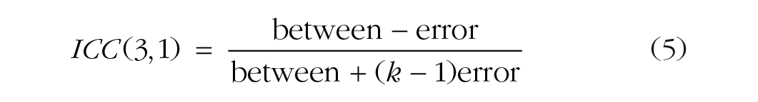
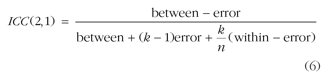
We have taken the liberty of replacing Koo and Li’s notation (distinguishing variance obtained within columns vs. within rows) with a between/within-subjects notation, in which “between” refers to between-subjects variance, “within” refers to within-subjects or between-sessions variance, and “error” refers to error variance; k is the number of measurements, and n is the sample size. Note that agreement (Equation 6) extends consistency (Equation 5) by including within-subjects variance (changes between tests) in the denominator. This causes the denominator to be larger if there is error associated with differences between sessions within subjects, which in turn results in a lower ICC estimate for agreement than for consistency.

ICCs (including 95% confidence intervals) can be estimated easily in R using the psych package (Revelle, 2018). The following code first loads the psych package before calling the ICC function. It selects the Stroop data from Hedge et al. (2018) from the two available time points: Stroop_1 and Stroop_2.

require(psych)

ICC(summary[,c(“Stroop_1”, “Stroop_2”)])

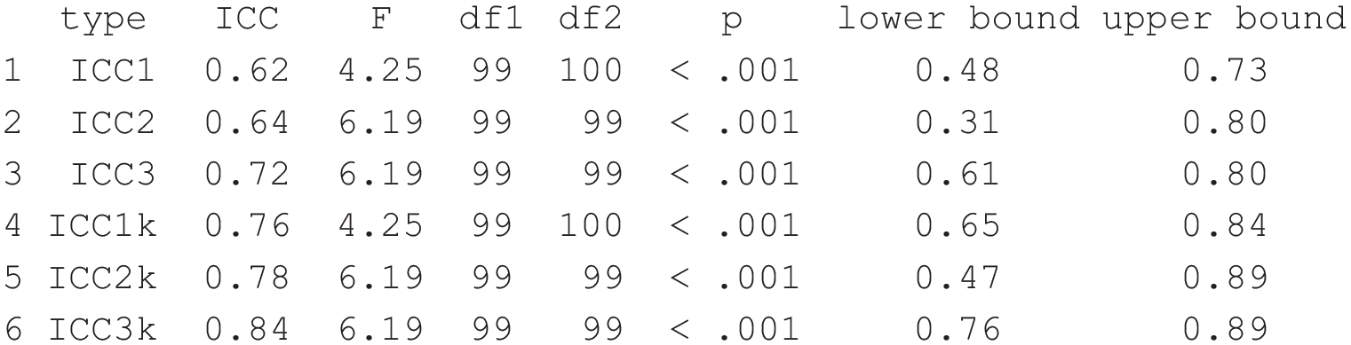
The standard output, shown in Figure 5, includes six variations of the ICC and related test statistics. The second and third rows of the output correspond to the ICC(2,1) (absolute agreement) and ICC(3,1) (consistency). The ICC column provides the test-retest reliability estimates, and the final two columns show the lower and upper bounds of the 95% confidence intervals around the point estimates.

Fig. 5.

R output showing the estimated intraclass correlation coefficients (ICCs) for the data from Hedge, Powell, and Sumner (2018). See the text for details. Note that this output has been altered slightly to be more presentable here.

The agreement and consistency estimates in this output might be reported as follows:

The Stroop task’s test-retest reliability between the first and second testing sessions was estimated with intraclass correlation coefficients (ICCs) using the psych package in R (Revelle, 2018). We report the results of two-way mixed-effects models for absolute agreement, ICC(2,1), and consistency, ICC(3,1). The estimated agreement was .64, 95% confidence interval (CI) = [.31, .80], and the estimated consistency was .72, 95% CI = [.61, .80].

Other recommendations

Our chief aim in this article is to argue for a culture change and to encourage researchers to adopt a standard practice of estimating and reporting the reliability of their measurements. There are several other related recommendations we would like to make.

First, we recommend that when developing novel computerized tasks (or adapting existing ones), researchers conduct validation studies for the new measures. This would greatly facilitate the development of reliable and valid measurements. Work such as this should be encouraged as an essential contribution to psychological science. Providing open data would further assist researchers in examining the reliability of cognitive measures whose reliability has not been reported and would provide opportunities to test different scoring approaches and examine any changes in the psychometrics of the outcome.

Second, we recommend that psychometric information be pooled so that researchers have access to a meta-archive tool. To adequately fill the current gap in knowledge, this pool would need to include psychometric information that has not yet been analyzed (or has gone unreported) in the existing literature. However, even collating already published psychometric information would allow researchers to compare, for example, the reliability estimate from a novel clinical sample with typically observed reliability estimates. Thus, researchers would not have to rely on thresholds for “adequate” or “good” reliability but would be able to directly compare their own reliability estimates with those typically observed for similar measures.

Finally, although most of our recommendations are aimed at researchers, it is the responsibility of journal editors and peer reviewers to request psychometric information on cognitive-behavioral tasks, just as they would for questionnaire measures. Extending current requirements for reporting effect sizes and confidence intervals, or precise p values, reviewers could request psychometric evaluations of all measures used, whether those measures are based on self-report or other behavioral data. Indeed, reporting the psychometric properties of measurements falls clearly within the American Psychological Association’s reporting standards (Appelbaum et al., 2018, p. 7).

Summary

We have argued that researchers using cognitive-behavioral measures should adopt a standard practice of estimating and reporting the reliability of these measures. We have discussed several issues that arise when a measure has low reliability, as well as difficulties in comparing effect-size estimates when reliability is unknown, and we have pointed out that reliability is so seldom reported that one cannot know the impact of these issues on the current state of knowledge. Beyond arguing that researchers need to report reliability estimates as standard practice, we have tried to help make this a reality by providing some assistance, in the form of a short tutorial and R code. Future researchers, especially those wanting to use a measure whose reliability in experimental settings has been tested only in their correlational research, will benefit if reporting reliability becomes standard. Today’s researchers have an obligation to future researchers to provide a sound evidence base, and this includes developing valid and reliable tools. For this to happen, psychological scientists must develop a research culture in which it is routine to estimate and report the reliability of cognitive-behavioral measures.

Supplemental Material

Parsons_AMPPSOpenPracticesDisclosure-v1.0 – Supplemental material for Psychological Science Needs a Standard Practice of Reporting the Reliability of Cognitive-Behavioral Measurements

Supplemental material, Parsons_AMPPSOpenPracticesDisclosure-v1.0 for Psychological Science Needs a Standard Practice of Reporting the Reliability of Cognitive-Behavioral Measurements by Sam Parsons, Anne-Wil Kruijt and Elaine Fox in Advances in Methods and Practices in Psychological Science

Footnotes

Acknowledgements

We would like to thank Craig Hedge for making the data used in our examples open and available. We would also like to thank all the people who provided feedback on the preprint version of this article. Their comments and critical feedback, and the articles they shared, have helped us develop this manuscript. In alphabetical order (apologies to anybody missed), we thank James Bartlett, Paul Christiansen, Oliver Clarke, Andrew Jones, Michael Kane, Jesse Kaye, Rogier Kievit, Kevin King, Mike Lawrence, Marcus Munafò, Cliodhna O’Connor, Oscar Olvera, Oliver Robinson, Guillaume Rousselet, Eric-Jan Wagenmakers, and Bruno Zumbo.

Action Editor

Pamela Davis-Kean served as action editor for this article.

Author Contributions

S. Parsons conceived and wrote the manuscript. A.-W. Kruijt provided crucial conceptual and theoretical feedback. All the authors provided critical input to develop the final manuscript, which they all agreed upon.

ORCID iDs

Sam Parsons

Anne-Wil Kruijt

Declaration of Conflicting Interests

The author(s) declared that there were no conflicts of interest with respect to the authorship or the publication of this article.

Funding

This work was funded by the European Research Council under the European Union’s Seventh Framework Programme (FP7/2007-2013) and European Research Council Grant 324176.

Open Practices

Open Data: not applicable

Open Materials:

Preregistration: not applicable

All materials have been made publicly available via the Open Science Framework and can be accessed at https://osf.io/9jp65/. The complete Open Practices Disclosure for this article can be found at http://journals.sagepub.com/doi/suppl/10.1177/2515245919879695. This article has received the badge for Open Materials. More information about the Open Practices badges can be found at .

Prior Versions

An earlier version of this manuscript was posted as a preprint on PsyArXiv ().

Notes

References

Appelbaum

Cooper

Kline

R. B.

Mayo-Wilson

Nezu

A. M.

Rao

S. M.

(2018). Journal article reporting standards for quantitative research in psychology: The APA Publications and Communications Board task force report. American Psychologist, 73, 3–25. doi:10.1037/amp0000191

Aust

Barth

(2018). papaja: Prepare APA journal articles with R Markdown (R package Version 0.1.0.9842) [Computer software]. Retrieved from https://github.com/crsh/papaja

Bar-Haim

Holoshitz

Eldar

Frenkel

T. I.

Muller

Charney

D. S.

. . . Wald

(2010). Life-threatening danger and suppression of attention bias to threat. American Journal of Psychiatry, 167, 694–698. doi:10.1176/appi.ajp.2009.09070956

Barry

A. E.

Chaney

Piazza-Gardner

A. K.

Chavarria

E. A.

(2014). Validity and reliability reporting practices in the field of health education and behavior: A review of seven journals. Health Education & Behavior, 41, 12–18. doi:10.1177/1090198113483139

Borsboom

Kievit

R. A.

Cervone

Hood

S. B.

(2009). The two disciplines of scientific psychology, or: The disunity of psychology as a working hypothesis. In Valsiner

Molenaar

P. C. M.

Lyra

M. C. D. P.

Chaudhary

(Eds.), Dynamic process methodology in the social and developmental sciences (pp. 67–97). New York, NY: Springer.

Brown

H. M.

Eley

T. C.

Broeren

MacLeod

Rinck

Hadwin

J. A.

Lester

K. J.

(2014). Psychometric properties of reaction time based experimental paradigms measuring anxiety-related information-processing biases in children. Journal of Anxiety Disorders, 28, 97–107. doi:10.1016/j.janxdis.2013.11.004

Brown

(1910). Some experimental results in the correlation of mental health abilities. British Journal of Psychology, 1904-1920, 3, 296–322. doi:10.1111/j.2044-8295.1910.tb00207.x

Button

Lewis

Penton-Voak

Munafò

(2013). Social anxiety is associated with general but not specific biases in emotion recognition. Psychiatry Research, 210, 199–207. doi:10.1016/j.psychres.2013.06.005

Champely

(2018). Pwr: Basic functions for power analysis (R package Version 1.2-2) [Computer software]. Retrieved from https://CRAN.R-project.org/package=pwr

10.

Cisler

J. M.

Koster

E. H. W.

(2010). Mechanisms of attentional biases towards threat in anxiety disorders: An integrative review. Clinical Psychology Review, 30, 203–216. doi:10.1016/j.cpr.2009.11.003

11.

Cooper

S. R.

Gonthier

Barch

D. M.

Braver

T. S.

(2017). The role of psychometrics in individual differences research in cognition: A case study of the AX-CPT. Frontiers in Psychology, 8, Article 1482. doi:10.3389/fpsyg.2017.01482

12.

Cronbach

L. J.

(1951). Coefficient alpha and the internal structure of tests. Psychometrika, 16, 297–334.

13.

Cronbach

L. J.

(1957). The two disciplines of scientific psychology. American Psychologist, 12, 671–684.

14.

Cronbach

L. J.

(1975). Beyond the two disciplines of scientific psychology. American Psychologist, 30, 116–127. doi:10.1037/h0076829

15.

Cronbach

L. J.

Hartmann

(1954). A note on negative reliabilities. Educational and Psychological Measurement, 14, 342–346. doi:10.1177/001316445401400213

16.

De Schryver

Hughes

Rosseel

De Houwer

. (2016). Unreliable yet still replicable: A comment on LeBel and Paunonen (2011). Frontiers in Psychology, 6, Article 2039. doi:10.3389/fpsyg.2015.02039

17.

Dunn

T. J.

Baguley

Brunsden

(2014). From alpha to omega: A practical solution to the pervasive problem of internal consistency estimation. British Journal of Psychology, 105, 399–412. doi:10.1111/bjop.12046

18.

Enock

P. M.

Hofmann

S. G.

McNally

R. J.

(2014). Attention bias modification training via smartphone to reduce social anxiety: A randomized, controlled multi-session experiment. Cognitive Therapy and Research, 38, 200–216. doi:10.1007/s10608-014-9606-z

19.

Enock

P. M.

Robinaugh

D. J.

Reese

H. E.

McNally

R. J.

(2012, November). Improved reliability estimation and psychometrics of the dot-probe paradigm on smartphones and PC. Poster session presented at the annual meeting of the Association of Behavioral and Cognitive Therapies, National Harbor, MD.

20.

Fisher

(1954). Statistical methods for research workers. Edinburgh, Scotland: Oliver and Boyd.

21.

Flake

J. K.

Pek

Hehman

(2017). Construct validation in social and personality research: Current practice and recommendations. Social Psychological and Personality Science, 8, 370–378. doi:10.1177/1948550617693063

22.

Gawronski

Deutsch

Banse

(2011). Response interference tasks as indirect measures of automatic associations. In Klauer

K. C.

Voss

Stahl

(Eds.), Cognitive methods in social psychology (pp. 78–123). New York, NY: Guilford Press.

23.

Gonthier

Macnamara

B. N.

Chow

Conway

A. R. A.

Braver

T. S.

(2016). Inducing proactive control shifts in the AX-CPT. Frontiers in Psychology, 7, Article 1822. doi:10.3389/fpsyg.2016.01822

24.

Gotlib

I. H.

Joormann

(2010). Cognition and depression: Current status and future directions. Annual Review of Clinical Psychology, 6, 285–312. doi:10.1146/annurev.clinpsy.121208.131305

25.

Hedge

Powell

Sumner

(2018). The reliability paradox: Why robust cognitive tasks do not produce reliable individual differences. Behavior Research Methods, 50, 1166–1186. doi:10.3758/s13428-017-0935-1

26.

Henry

Wickham

(2019). Purrr: Functional programming tools (R package Version 0.3.2) [Computer software]. Retrieved from https://CRAN.R-project.org/package=purrr

27.

Hussey

Hughes

(2018). Hidden invalidity among fifteen commonly used measures in social and personality psychology. PsyArXiv. doi:10.31234/osf.io/7rbfp

28.

Ioannidis

J. P. A.

(2005). Why most published research findings are false. PLOS Medicine, 2(8), Article e124. doi:10.1371/journal.pmed.0020124

29.

Ioannidis

J. P. A.

Tarone

McLaughlin

J. K.

(2011). The false-positive to false-negative ratio in epidemiologic studies. Epidemiology, 22, 450–456. doi:10.1097/EDE.0b013e31821b506e

30.

Jones

Christiansen

Field

(2018). Failed attempts to improve the reliability of the alcohol visual probe task following empirical recommendations. Psychology of Addictive Behaviors, 32, 922–932. doi:10.31234/osf.io/4zsbm

31.

Kanyongo

G. Y.

Brook

G. P.

Kyei-Blankson

Gocmen

(2007). Reliability and statistical power: How measurement fallibility affects power and required sample sizes for several parametric and nonparametric statistics. Journal of Modern Applied Statistical Methods, 6, 81–90. doi:10.22237/jmasm/1177992480

32.

Kappenman

E. S.

Farrens

J. L.

Luck

S. J.

Proudfit

G. H.

(2014). Behavioral and ERP measures of attentional bias to threat in the dot-probe task: Poor reliability and lack of correlation with anxiety. Frontiers in Psychology, 5, Article 1368. doi:10.3389/fpsyg.2014.01368

33.

Koo

T. K.

M. Y.

(2016). A guideline of selecting and reporting intraclass correlation coefficients for reliability research. Journal of Chiropractic Medicine, 15, 155–163. doi:10.1016/j.jcm.2016.02.012

34.

Kruijt

A.-W.

Field

A. P.

Fox

(2016). Capturing dynamics of biased attention: Are new attention variability measures the way forward? PLOS ONE, 11(11), Article e0166600. doi:10.1371/journal.pone.0166600

35.

LeBel

E. P.

Paunonen

S. V.

(2011). Sexy but often unreliable: The impact of unreliability on the replicability of experimental findings with implicit measures. Personality and Social Psychology Bulletin, 37, 570–583. doi:10.1177/0146167211400619

36.

Love

Selker

Marsman

Jamil

Dropmann

Verhagen

. . . Wagenmakers

E.-J.

(2019). JASP: Graphical statistical software for common sta-tistical designs. Journal of Statistical Software, 88(2). doi:10.18637/jss.v088.i02

37.

Luck

S. J.

(2019, February 19). Why experimentalists should ignore reliability and focus on precision [Blog post]. Retrieved from https://lucklab.ucdavis.edu/blog/2019/2/19/reliability-and-precision

38.

MacLeod

Grafton

(2016). Anxiety-linked attentional bias and its modification: Illustrating the importance of distinguishing processes and procedures in experimental psychopathology research. Behaviour Research and Therapy, 86, 68–86. doi:10.1016/j.brat.2016.07.005

39.

MacLeod

Mathews

Tata

(1986). Attentional bias in emotional disorders. Journal of Abnormal Psychology, 95, 15–20.

40.

MacLeod

C. M.

(1991). Half a century of research on the Stroop effect: An integrative review. Psychological Bulletin, 109, 163–203.

41.

MacLeod

J. W.

Lawrence

M. A.

McConnell

M. M.

Eskes

G. A.

Klein

R. M.

Shore

D. I.

(2010). Appraising the ANT: Psychometric and theoretical considerations of the Attention Network Test. Neuropsychology, 24, 637–651. doi:10.1037/a0019803

42.

Marsman

Wagenmakers

E.-J.

(2017). Bayesian benefits with JASP. European Journal of Developmental Psychology, 14, 545–555. doi:10.1080/17405629.2016.1259614

43.

Marwick

(2019). Wordcountaddin: Word counts and readability statistics in R markdown documents (R package Version 0.3.0.9000) [Computer software]. Retrieved from https://github.com/benmarwick/wordcountaddin

44.

McGraw

K. O.

Wong

S. P.

(1996). Forming inferences about some intraclass correlation coefficients. Psychological Methods, 1, 30–46.

45.

Michalke

(2018a). koRpus: An R package for text analysis (R package Version 0.11-5) [Computer software]. Re-trieved from https://reaktanz.de/?c=hacking&s=koRpus

46.

Michalke

(2018b). sylly: Hyphenation and syllable counting for text analysis (R package Version 0.1-5) [Computer software]. Retrieved from https://reaktanz.de/?c=hacking&s=sylly

47.

Michalke

(2019). koRpus.lang.en: Language support for ‘koRpus’ package: English (R package Version 0.1-3) [Computer software]. Retrieved from https://undocumeantit.github.io/repos/l10n/pckg/koRpus.lang.en/index.html

48.

Morey

R. D.

Lakens

(2016). Why most of psychology is statistically unfalsifiable. Retrieved from https://github.com/richarddmorey/psychology_resolution/blob/master/paper/response.pdf

49.

Müller

Wickham

(2019). tibble: Simple data frames (R package Version 2.1.3) [Computer software]. Retrieved from https://CRAN.R-project.org/package=tibble

50.

Parsons

(2019a). splithalf package documentation. Retrieved from https://sdparsons.github.io/splithalf_documentation/

51.

Parsons

(2019b). splithalf: Robust estimates of split half reliability (R package Version 5) [Computer software]. doi:10.6084/m9.figshare.5559175.v5

52.

Peters

G.-J. Y.

(2014). The alpha and the omega of scale reliability and validity: Why and how to abandon Cronbach’s alpha and the route towards more comprehensive assessment of scale quality. European Health Psychology, 16, 56–69.

53.

Price

R. B.

Kuckertz

J. M.

Siegle

G. J.

Ladouceur

C. D.

Silk

J. S.

Ryan

N. D.

. . . Amir

(2015). Empirical recommendations for improving the stability of the dot-probe task in clinical research. Psychological Assessment, 27, 365–376. doi:10.1037/pas0000036

54.

R Core Team. (2018). R: A language and environment for statistical computing. Vienna, Austria: R Foundation for Statistical Computing.

55.

Revelle

(2018). psych: Procedures for psychological, psychometric, and personality research (R package Version 1.8.12) [Computer software]. Retrieved from https://CRAN.R-project.org/package=psych

56.

Richmond

L. L.

Redick

T. S.

Braver

T. S.

(2016). Remembering to prepare: The benefits (and costs) of high working memory capacity. Journal of Experimental Psychology: Learning, Memory, and Cognition, 41, 1764–1777. doi:10.1037/xlm0000122

57.

Rodebaugh

T. L.

Scullin

R. B.

Langer

J. K.

Dixon

D. J.

Huppert

J. D.

Bernstein

. . . Lenze

E. J.

(2016). Unreliability as a threat to understanding psychopathology: The cautionary tale of attentional bias. Journal of Abnormal Psychology, 125, 840–851. doi:10.1037/abn0000184

58.

Rouder

J. N.

Haaf

J. M.

(2018a). Power, dominance, and constraint: A note on the appeal of different design traditions. Advances in Methods and Practices in Psychological Science, 1, 19–26.

59.

Rouder

J. N.

Haaf

J. M.

(2018b). A psychometrics of individual differences in experimental tasks. PsyArXiv. doi:10.31234/osf.io/f3h2k

60.

Rouder

J. N.

Kumar

Haaf

J. M.

(2019). Why most studies of individual differences with inhibition tasks are bound to fail. PsyArXiv. doi:10.31234/osf.io/3cjr5

61.

Schmidt

F. L.

Hunter

J. E.

(1996). Measurement error in psychological research: Lessons from 26 research scenarios. Psychological Methods, 1, 199–223.

62.

Schmukle

S. C.

(2005). Unreliability of the dot probe task. European Journal of Personality, 19, 595–605. doi:10.1002/per.554

63.

Shrout

P. E.

Fleiss

J. L.

(1979). Intraclass correlations: Uses in assessing rater reliability. Psychological Bulletin, 86, 420–428.

64.

Sigurjónsdóttir

Ó.

Sigurðardóttir

Björnsson

A. S.

Kristjánsson

. (2015). Barking up the wrong tree in attentional bias modification? Comparing the sensitivity of four tasks to attentional biases. Journal of Behavior Therapy and Experimental Psychiatry, 48, 9–16. doi:10.1016/j.jbtep.2015.01.005

65.

Sijtsma

(2009). On the use, the misuse, and the very limited usefulness of Cronbach’s alpha. Psychometrika, 74, 107–120. doi:10.1007/s11336-008-9101-0

66.

Slaney

K. L.

Tkatchouk

Gabriel

S. M.

Maraun

M. D.

(2009). Psychometric assessment and reporting practices: Incongruence between theory and practice. Journal of Psychoeducational Assessment, 27, 465–476. doi:10.1177/0734282909335781

67.

Spearman

(1904). The proof and measurement of association between two things. The American Journal of Psychology, 15, 72–101. doi:10.2307/1412159

68.

Spearman

(1910). Correlation calculated from faulty data. British Journal of Psychology, 1904-1920, 3, 271–295. doi:10.1111/j.2044-8295.1910.tb00206.x

69.

Staugaard

S. R.

(2009). Reliability of two versions of the dot-probe task using photographic faces. Psychology Science Quarterly, 51, 339–350.

70.

Strauss

M. E.

McLouth

C. J.

Barch

D. M.

Carter

C. S.

Gold

J. M.

Luck

S. J.

. . . Silverstein

S. M.

(2014). Temporal stability and moderating effects of age and sex on CNTRaCS task performance. Schizophrenia Bulletin, 40, 835–844. doi:10.1093/schbul/sbt089

71.

Stroop

J. R.

(1935). Studies of interference in serial verbal reactions. Journal of Experimental Psychology, 18, 643–662.

72.

Vacha-Haase

Henson

R. K.

Caruso

J. C.

(2002). Reliability generalization: Moving toward improved understanding and use of score reliability. Educational and Psychological Measurement, 62, 562–569. doi:10.1177/0013164402062004002

73.

Vasey

M. W.

Dalgleish

Silverman

W. K.

(2003). Research on information-processing factors in child and adolescent psychopathology: A critical commentary. Journal of Clinical Child & Adolescent Psychology, 32, 81–93. doi:10.1207/S15374424JCCP3201_08

74.

Viladrich

Angulo-Brunet

Doval

(2017). A journey around alpha and omega to estimate internal consistency reliability. Anales de Psicología/Annals of Psychology, 33, 755–782. doi:10.6018/analesps.33.3.268401

75.

Waechter

Nelson

A. L.

Wright

Hyatt

Oakman

(2014). Measuring attentional bias to threat: Reliability of dot probe and eye movement indices. Cognitive Therapy and Research, 38, 313–333. doi:10.1007/s10608-013-9588-2

76.

Waechter

Stolz

J. A.

(2015). Trait anxiety, state anxiety, and attentional bias to threat: Assessing the psychometric properties of response time measures. Cognitive Therapy and Research, 39, 441–458. doi:10.1007/s10608-015-9670-z

77.

Wagenmakers

E.-J.

Love

Marsman

Jamil

Verhagen

. . . Morey

R. D.

(2018). Bayesian inference for psychology. Part II: Example applications with JASP. Psychonomic Bulletin & Review, 25, 58–76. doi:10.3758/s13423-017-1323-7

78.

Wickham

(2016). ggplot2 (R package Version 3.2.0) [Computer software]. Retrieved from https://ggplot2.tidyverse.org

79.

Wickham

(2017). tidyverse: Easily install and load the ‘tidyverse’ (R package Version 1.2.1) [Computer soft-ware]. Retrieved from https://CRAN.R-project.org/package=tidyverse

80.

Wickham

(2019a). forcats: Tools for working with categorical variables (factors) (R package Version 0.4.0) [Computer software]. Retrieved from https://CRAN.R-project.org/package=forcats

81.

Wickham

(2019b). stringr: Simple, consistent wrappers for common string operations (R package Version 1.4.0) [Computer software]. Retrieved from https://CRAN.R-project.org/package=stringr

82.

Wickham

François

Henry

Müller

(2019). dplyr: A grammar of data manipulation (R package Version 0.8.3) [Computer software]. Retrieved from https://CRAN.R-project.org/package=dplyr

83.

Wickham

Henry

(2019). tidyr: tidy messy data (R package Version 0.8.3) [Computer software]. Retrieved from https://CRAN.R-project.org/package=tidyr

84.

Wickham

Hester

Francois

(2018). readr: Read rectangular text data (R package Version 1.3.1) [Computer software]. Retrieved from https://CRAN.R-project.org/package=readr

85.

Wilkinson

& Task Force on Statistical Inference, American Psychological Association, Science Directorate. (1999). Statistical methods in psychology journals: Guidelines and explanations. American Psychologist, 54, 594–604.

86.

Xie

(2019). formatR: Format R code automatically (R package Version 1.7) [Computer software]. Retrieved from https://CRAN.R-project.org/package=formatR

87.

Xie

Allaire

J. J.

(2019). tufte: tufte’s styles for R Markdown documents (R package Version 0.5) [Computer software]. Retrieved from https://CRAN.R-project.org/package=tufte

88.

Yiend

(2010). The effects of emotion on attention: A review of attentional processing of emotional information. Cognition & Emotion, 24, 3–47. doi:10.1080/02699930903205698

89.

Zimmerman

D. W.

Zumbo

B. D.

(2015). Resolving the issue of how reliability is related to statistical power: Adhering to mathematical definitions. Journal of Modern Applied Statistical Methods, 14(2), 9–26. doi:10.22237/jmasm/1446350640

Supplementary Material

Please find the following supplemental material available below.

For Open Access articles published under a Creative Commons License, all supplemental material carries the same license as the article it is associated with.

For non-Open Access articles published, all supplemental material carries a non-exclusive license, and permission requests for re-use of supplemental material or any part of supplemental material shall be sent directly to the copyright owner as specified in the copyright notice associated with the article.

0.00 MB

0.64 MB