Sage Journals: Discover world-class research

Abstract

In psychology, researchers are often interested in the predictive classification of individuals. Various models exist for such a purpose, but which model is considered a best practice is conditional on attributes of the data. Under certain conditions, linear discriminant analysis (LDA) has been shown to perform better than other predictive methods, such as logistic regression, multinomial logistic regression, random forests, support-vector machines, and the K-nearest neighbor algorithm. The purpose of this Tutorial is to provide researchers who already have a basic level of statistical training with a general overview of LDA and an example of its implementation and interpretation. Decisions that must be made when conducting an LDA (e.g., prior specification, choice of cross-validation procedures) and methods of evaluating case classification (posterior probability, typicality probability) and overall classification (hit rate, Huberty’s I index) are discussed. LDA for prediction is described from a modern Bayesian perspective, as opposed to its original derivation. A step-by-step example of implementing and interpreting LDA results is provided. All analyses were conducted in R, and the script is provided; the data are available online.

Keywords

discriminant analysis machine learning classification R Bayesian analysis open materials

In psychology, researchers are often interested in predicting the classification of individuals. For example, accurately predicting who will drop out of a program can make it possible to avoid fruitless expenses, and predicting the severity of an illness can aid appropriate referral to treatment. Such prediction typically involves a set of predictor variables (e.g., demographics, condition-related covariates) and a categorical outcome with two or more mutually exclusive groups (e.g., people who survive to a certain date vs. those who do not; patients with mild, moderate, or severe depression). Several parametric and nonparametric methods for making predictive classifications are available. Classic parametric methods include linear discriminant analysis (LDA) and quadratic discriminant analysis (QDA), whereas nonparametric methods include variants of the K-nearest neighbors algorithm, support-vector machines, random forests, and neural networks. Notably, Hastie, Tibshirani, and Friedman (2009) stated that, in comparison with more modern nonparametric methods, “both LDA and QDA perform well on an amazingly large and diverse set of classification tasks. . . . It seems that whatever exotic tools are the rage of the day, we should always have available these two simple tools” (p. 111). The purpose of this article is to provide an introduction to the application of LDA for prediction in a Bayesian framework, review best-practice recommendations, and detail an example of the method’s application. Note that although LDA may also be used for description, our focus is on the application of LDA for prediction.

Disclosures

All the analyses for the example application of LDA were conducted in R (R Core Team, 2018). The syntax is provided in Appendix A and is available at the Open Science Framework (https://osf.io/6bk24/files/). The data are available online (UCLA Institute for Digital Research and Education, 2017).

Two Purposes of LDA

Fisher (1936) originally developed LDA as a method for finding linear combinations of variables that best separated observations into groups, or classifications. Using these linear combinations, researchers can learn which of the variables contribute most to group separation and the likely classification of a case with unobserved group membership. For example, clinical psychologists may be interested in associations between their clients’ psychological characteristics at intake (e.g., stress tolerance, anxiety, and self-confidence) and their compliance with treatment (e.g., missing most sessions, missing a few sessions, or missing no sessions); LDA can be used to identify which psychological characteristics contribute most to treatment compliance, as well as to formulate a model for using these characteristics to predictively classify treatment compliance among future clients. Fisher used the same method for both purposes, but LDA was subsequently modified for use in prediction. Given this differentiation between two purposes—description (also termed discrimination or separation) and prediction (also termed classification or allocation; Johnson & Wichern, 2007)—some researchers have named the two methods differentially as well.

When LDA is used to describe group differences on a set of variables, the method is often referred to as descriptive discriminant analysis (DDA). More specifically, DDA is used to describe which of a set of variables contribute most to group differentiation. It is suitable, for instance, as a follow-up to a statistically significant multivariate analysis of variance (Enders, 2003; Warne, 2014). The researcher estimates linear discriminant functions (LDFs), each of which is used to create discriminant scores explaining variability between groups. Plotting the linear discriminant scores can help researchers visualize the data in a lower-dimensional space, and plotting the coefficients of the LDFs can help researchers understand the dimensions that best separate the groups.

Alternatively, when LDA is used to develop classification rules for predicting group membership of new cases with unknown classification, it is often referred to as predictive discriminant analysis (PDA; e.g., Huberty & Hussein, 2003; Huberty & Olejnik, 2006). In this approach, a separate linear classification function (LCF) is derived for each group. (Although Hastie et al., 2009, called LCFs linear discriminant functions, we follow the terminology of Huberty and Hussein, 2003.) The data for a case with unknown classification are submitted to these LCFs, and the results are used to predict classification. For example, a sample of adolescents who have experienced a traumatic event may be classified into groups of low, medium, or high severity of posttraumatic stress disorder (PTSD) symptoms. A predictive model (set of LCFs) derived using these cases with observed group membership may then be used to predict the classification of symptom severity for a child who experiences a similar traumatic event.¹ LDA for prediction, our focus in this article, is the same as PDA; these terms can be used interchangeably in this context.

The differentiation between DDA and PDA is more than semantic. In DDA, the original method presented by Fisher (1936) is used to estimate LDFs, whereas in PDA, the LCFs are derived with the additional influence of prior information, within a Bayesian framework. Welch (1939) formally incorporated this use of prior information in conjunction with Fisher’s (1936) original derivation to achieve optimal predictive classification (Hastie et al., 2009).

Though Welch (1939) did not expressly describe his work as Bayesian, the procedure is the same. The Bayesian derivation of LDA for classification provides posterior probabilities of a case’s membership in the groups under consideration. A single case will have a posterior probability of membership for each group (e.g., .10 for Group 1, .24 for Group 2, and .66 for Group 3), and these probabilities will sum to 1.00 across groups. Each posterior probability is the probability that the case in question, given the observed data for that case, is a member of the given group, characterized by the data of the group’s members. Posterior probabilities may be useful when the classification of a case is less than clear-cut (Johnson & Wichern, 2007). A Bayesian derivation of LDA for classification utilizes prior probabilities of group membership—in conjunction with the observed variables—to produce these posterior probabilities. Prior probabilities, for example, can be based on what is already known about the population distribution. If there are two possible classifications (e.g., successful or unsuccessful treatment), and one classification group has contained only 5% of cases in the past, the analyst would want to classify a case into that low-occurrence group only when the evidence for doing so is very strong (Klecka, 1980). In this case, the prior probability for the low-occurrence group could be set to .05, and the prior probability for the other group could be .95, to reflect the known population distribution. When the prior probability of group membership is equal across groups and the assumptions of LDA (discussed later) are met, Fisher’s and Welch’s derivations will yield the same results for classification (Huberty & Hussein, 2003).

Whereas our focus in this article is on the Bayesian application, readers who are interested in the original approach may want to consult Fisher (1936) or Johnson and Wichern (2007) for more detail. Kruschke has provided explanations of applied Bayesian estimation with t tests (Kruschke, 2013) and regression (Kruschke, Aguinis, & Joo, 2012), and an explanation of applied Bayesian estimation with multilevel modeling is available in Boedeker (2017). Appendix B provides more technical details on the derivation of LCFs.

Overview of LDA for Prediction

LDA can be used for allocating new observations to previously defined categories through the creation of a classification rule (Huberty, 1994; Huberty & Barton, 1989; Klecka, 1980). First, data for which group membership is known (training data) are used to derive LCFs. LCFs are similar to unstandardized regression equations; the sum of an intercept and the products of weights and observed variables produce a single classification score. LCFs are derived using Mahalanobis distance and prior probability. Mahalanobis distance is a single value describing the distance between two points in multivariate space. In classification, these two points are the location of a case’s data and a given group’s centroid, that is, the group’s average for each variable used for classification within that group. A Mahalanobis distance can be calculated for each case for each group. The group with the lowest Mahalanobis distance from a case is the group to which the case is most similar in multivariate space.

A case’s observations are submitted to each group’s LCF to calculate a classification score, and the case is assigned to the group for which it has the highest score. Posterior probabilities are also derived from these classification scores by using Bayes theorem. Posterior probabilities of membership in the groups and typicality probabilities—values representing how “typical” a case’s data are for each group—are used to evaluate the assigned classification.

The overall accuracy of prediction can be evaluated for the training data using hit rates and effect size (Huberty’s I index). Hit rate is the percentage of cases correctly predicted using the LCFs. Higher hit rates indicate more accurate prediction of group membership. Ultimately, if a set of LCFs is found to be accurate (i.e., the hit rate and Huberty’s I are high), it can be used to predict classification for a different set of cases for which group membership is unknown.

Specification of prior probability

In this section, we briefly describe four methods for specifying prior probabilities: (a) assuming equality across groups, (b) assuming equality to the data distribution, (c) using a known population distribution, and (d) using the cost of misclassification. The first method essentially admits no prior information about differences in group membership. In the two-group case, the prior probability of membership in Group 1 and the prior probability of membership in Group 2 would both equal .50 (i.e., 50%). With this method, the data entirely determine the posterior probabilities of group membership. Alternatively, the researcher may assume that the sample reflects the distribution of cases in the population and set the prior probabilities to reflect the percentages of group membership in the data. For instance, when this second method is used, if 30% of patients in the training data were classified as treatment seeking, then the prior probability for membership in the treatment-seeking group would be set to .30. If the analyst has prior knowledge of the distribution in the population, the third method can be used. That is, the assigned prior probabilities can reflect this knowledge. For example, prevalence of current PTSD is estimated at 3.5% in the general population (Kessler, Chiu, Demler, Merikangas, & Walters, 2005), so a researcher interested in evaluating a predictive model for identifying PTSD might set the prior probability of membership in a “current PTSD” group to .035. Finally, prior probabilities may be based on the cost of misclassification. Cancer diagnoses provide an example of when this approach is useful. Inaccurately classifying a tumor as benign is more lethal than inaccurately classifying it as malignant. If it is possible to numerically determine the costs of misclassification, then this information may be utilized in the prior probability.

Assumptions

Two assumptions of LDA for prediction are multivariate normality of the distribution of variables within classifications and equality of variance-covariance matrices across classifications. Both of these assumptions are reflected in Appendix B’s derivation of LCFs, which specifies that the data follow a multivariate normal distribution and pools the variance-covariance matrices across classes. Multivariate normality is particularly important for the utility of computed posterior probabilities and in calculating the intercept term of each LCF (Hastie et al., 2009). When multivariate normality is violated, the probabilities are not exact and must be interpreted with caution (Klecka, 1980; Lachenbruch, 1975). However, LDA results have been shown to be robust to violations of multivariate normality (Khondoker, Dobson, Skirrow, Simmons, & Stahl, 2016; Sherry, 2006), particularly when groups are approximately equal in size (Lachenbruch, 1975). The assumption of equal variance-covariance matrices is what makes LDA linear instead of quadratic (Huberty & Curry, 1978). In LDA, the LCF for each group is found using the pooled variance-covariance matrix, whereas in QDA, each group’s LCF is calculated using the group’s unique variance-covariance matrix (Huberty & Barton, 1989; Joachimsthaler & Stam, 1988).

When to use LDA for prediction

As we mentioned earlier, there are many methods for predictive classification. Recent simulation studies point to which methods perform best under various conditions.² For example, Khondoker et al. (2016) conducted a simulation comparing random forests, support-vector machines, LDA, and the K-nearest neighbor algorithm and found that none of these options performed uniformly best. However, when the number of predictors was less than half the sample size and the predictors had relatively high correlations (> .6; though not so high as to cause multicollinearity issues), LDA was the method of choice. Khondoker et al. provided further recommendations as to which classification method performs best in other data conditions as well, and we encourage readers who find themselves with data that are not well suited for LDA to consult that work. In another comparison of classifiers—including random forests, support-vector machines, and the K-nearest neighbor algorithm—LDA was shown to perform well when class membership was highly unbalanced (Brown & Mues, 2012).

Additionally, LDA may be preferable to logistic regression and multinomial logistic regression for group classification. More specifically, LDA can be used for classification of three or more groups (unlike logistic regression) and does not require specification of a reference group (unlike multinomial logistic regression). LDA also has the advantage that it can be used to estimate model parameters under conditions of separability (Hastie et al., 2009), that is, when a single predictor is able to perfectly separate cases into classes. If such separability occurs, the maximum likelihood estimator in logistic and multinomial logistic regression will fail to converge and will not produce accurate parameter estimates.

There are certain instances in which LDA may not perform optimally. For example, when data are not multivariate normal and the variance-covariance matrices are not approximately equal, LDA will not be optimal for classification. Either parametric or nonparametric classification methods that do not require explicit specification of data distributions may be more appropriate under such circumstances. Explanation of each of the alternative classification methods and why they may outperform LDA under various data conditions is beyond the scope of this Tutorial but is available in other sources (e.g., Hastie et al., 2009).

Model Evaluation

Case classification

A model’s case classification is evaluated using posterior and typicality probabilities. A case’s posterior probability for a given group indicates the certainty of that case’s classification in that group. For instance, if there are two groups (i.e., Group 1 and Group 2), and the posterior probabilities for a case belonging to those groups are .01 and .99, respectively, the evidence is strong that the case is a member of Group 2. If instead the posterior probabilities are .49 and .51, then the case’s membership in Group 2 is questionable. Such a case is considered a fence rider; its classification is in doubt because it has approximately equal posterior probabilities for multiple groups (Huberty & Olejnik, 2006). In LDA, fences are the thresholds that determine which cases get classified into which groups. As the observations closest to these fences, fence riders are the cases whose classification is most likely to be affected by outlier data, the inclusion or exclusion of new predictor variables, or failure to meet assumptions. Additionally, the presence of a large number of fence riders may suggest the possibility of another level of the grouping variable (e.g., a third group between two identified groups; Huberty & Olejnik, 2006). For example, a large number of fence riders between a “mild substance use” group and a “severe substance use” group may indicate the presence of a “moderate substance use” group in the training data.

The typicality probability is the “probability that a case that far from the centroid would actually belong to [the] group” (Klecka, 1980, p. 45); it indicates how typical an individual’s score is for a given group. Typicality probability is based on the right tail of the chi-square distribution; the chi-square value is equal to the Mahalanobis distance, and the degrees of freedom is equal to the number of predictors (Klecka, 1980). Generally, a larger distance indicates that an individual is less typical of the group (and has a lower typicality probability); conversely, a shorter distance indicates that a case is more typical of the group (and has a larger typicality probability). However, it is important to note that a small typicality probability for a given group does not necessarily mean that an individual should not be assigned to that group. Rather, the individual is potentially an outlier in the data set.

Overall classification

The overall accuracy of prediction (hit rate) in the training data is used to evaluate the utility of the prediction model (LCFs). However, the hit rate for LDA models is inherently biased—in most cases, artificially inflated. This bias comes from using LCFs to reclassify the same data set from which they were derived, a process known as internal classification. Methodologists have suggested that LDA hit rates should be calculated using external classification, that is, by calculating LCFs in one data set and then using those functions to classify cases in another data set (Hsu, 1989; Huberty, 1994; Huberty & Barton, 1989).

When external classification is not possible, cross-validation (CV) methods can be used to give an unbiased estimate of the hit rate. Three options are leave-one-out (LOO) CV, k-fold CV, and repeated k-fold CV. LOO CV is a jackknifing methodology. The classification functions are estimated with one observation held out, and then the held-out observation is classified (Lachenbruch & Mickey, 1968). This process is repeated for all cases. In the k-fold CV procedure, the sample is randomly divided into k subsets. The classification functions are derived using all but one subset, and the cases in the held-out subset are then classified. This is repeated for each of the subsets, and the hit rates are averaged across repetitions. In repeated k-fold CV, the k-fold procedure is repeated a specified number of times, each time with a different division of the sample into k subsets. The results over repetitions are averaged.

Hit rates obtained using CV methods are typically lower than the original hit rates, but are less biased estimates of classification accuracy and, therefore, are the hit rates that should be reported and interpreted. Rodriguez, Perez, and Lozano (2010) recommended using (a) k-fold CV with 5 or 10 folds in preference to LOO CV and (b) repeated k-fold CV in preference to k-fold and LOO CV. This recommendation was based on their simulation, in which LOO CV, though least biased, had the greatest variance in error estimation as well as the greatest computational cost. Though computational cost may not be an issue in applications in psychology, Hastie et al. (2009) recommended the k-fold procedure with 5 or 10 folds as a compromise between reducing estimator bias and reducing variance. In a simulation that varied sample size, Braga-Neto and Dougherty (2004) found that repeated k-fold CV with 10 folds performed well with as few as 20 cases. After CV, the final set of LCFs to be applied to data with unknown classification are the LCFs derived using the entire training data set.

Interpreting the hit rate without providing some context for the likelihood of accurate classification by chance can be misleading. For example, a hit rate of 80% may appear impressive at face value, but if 90% of the data were observed within one group, a hit rate of 80% would be less accurate than classification based solely on chance. Huberty and Lowman (2000) proposed Huberty’s I index as a measurement of improvement over chance. The chance hit rate, H_c, is calculated as follows:

H_{c} = \frac{\sum^{} q_{i} n_{i}}{N},

(1)

where q_i is the prior probability for group i, n_i is the number of cases in group i, and N is the total number of cases in the sample. In LDA for prediction, Huberty’s I index is considered the “gold standard” measure of effect size and is highly correlated with other measures of effect size (e.g., η²; Huberty & Lowman, 2000). Huberty’s I is calculated as follows:

I = \frac{H_{o} - H_{c}}{1 - H_{c}},

(2)

where H_o is the observed hit rate and H_c is the chance hit rate (Equation 1).

It is noteworthy that LDA differs from other methods with regard to the additive influence of new predictors. In other methods (e.g., multiple regression), the addition of a predictor will always lead to equal or greater accuracy in prediction. In LDA, that is not always the case; the addition of unrelated variables, or variables with extremely high collinearity, can reduce correct classification (Henson, 2002). Therefore, variables should be carefully selected and justified.

Example

In this section, we detail how to use LDA for classification in R. Annotated syntax for this example is available in Appendix A. The data were collected from a large international airline company and can be found online (UCLA Institute for Digital Research and Education, 2017). The data come from a project undertaken by industrial-organizational psychologists who were interested in whether three job classifications (Customer Service, Mechanic, and Dispatcher) appealed to different personality types. Possible predictive personality variables were assessed in 244 airline employees using a brief battery that asked questions about outdoor skills, social skills, and conservativeness.

Assumptions

Within each job classification, we assessed multivariate normality with scatterplots showing the association between squared Mahalanobis distance and associated chi-square quantiles (Fig. 1; Henson, 1999). For multivariate normality, plotted values are expected to fall generally on a diagonal. All three plots indicated some deviation from multivariate normality. The deviations of the Mechanics group were the greatest, although they did not appear to be extreme for the vast majority of cases. Additionally, we used Mardia’s (1970, 1974) skewness and kurtosis tests to evaluate multivariate normality (see Table 1). Combining the evidence from the plots and the null findings of the statistical tests, we determined that it was acceptable to assume that the distributions within each class were approximately multivariate normal. We assessed the equality of variance-covariance matrices with Box’s (1949) M and comparison of log determinants and their 95% confidence intervals (Cai, Liang, & Zhou, 2015). Box’s M was not statistically significant, based on the recommended lower criterion for statistical significance with this test (i.e., p < .001; Tabachnick & Fidell, 2013). A log determinant is essentially a single-value summary of the total variability within a matrix. Near equality between log determinants indicates that variability across matrices is similar (Tabachnick & Fidell, 2013). The log determinants across the three groups were similar, and their 95% confidence intervals overlapped (see Table 1). These findings indicated that the data did not violate any testable assumptions to an extent that would be concerning.

Fig. 1.

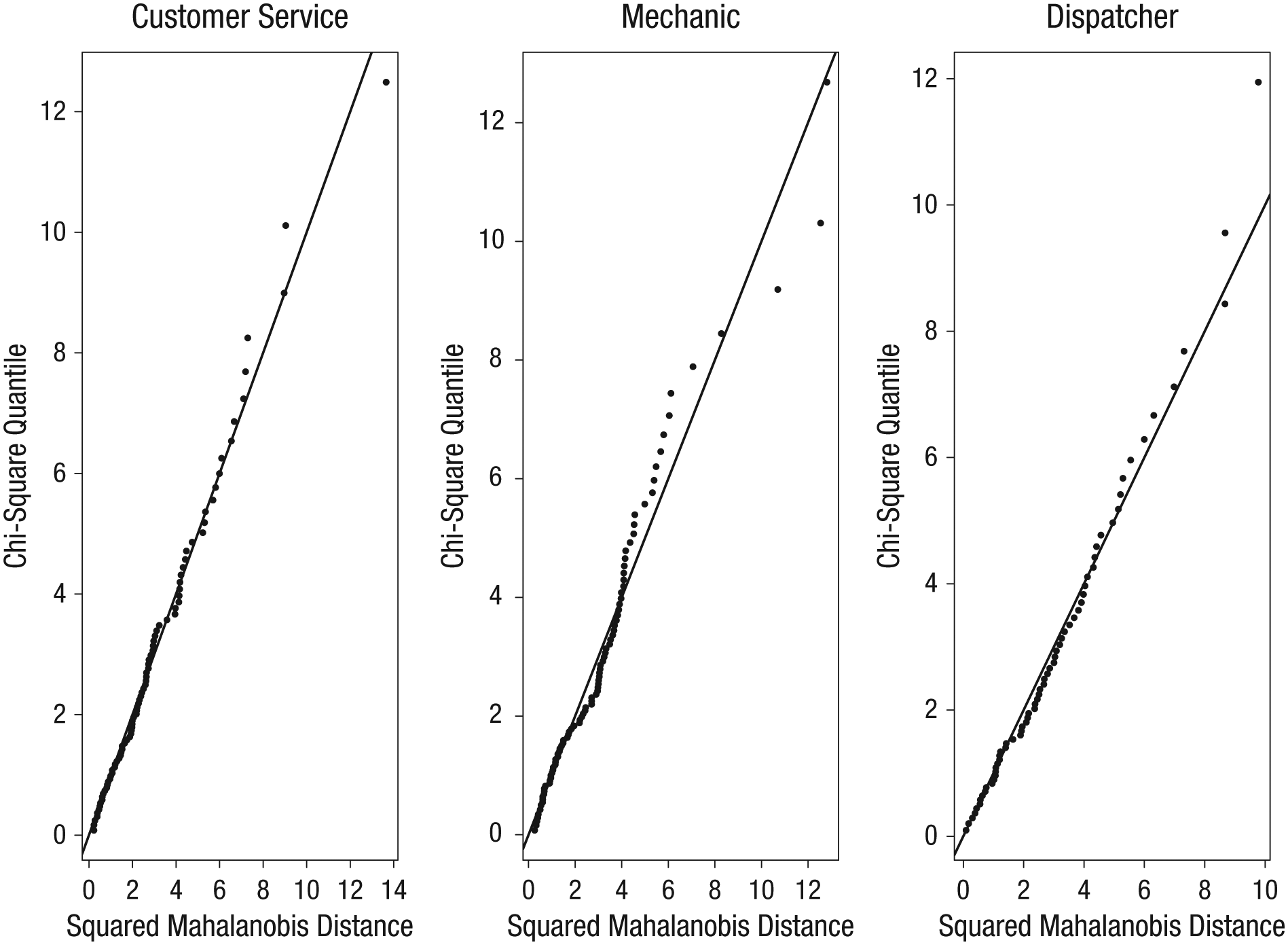
Scatterplots for assessing the multivariate normality of the predictor variables within each job classification (from left to right): Customer Service, Mechanic, and Dispatcher. The horizontal axis is the squared Mahalanobis distance, or multivariate distance, of the case from the centroid of the respective group, and the vertical axis is the case’s expected quantile in the chi-square distribution with degrees of freedom equal to the number of predictors.

Table 1.

Results of Assumption Checks for the Example Application of Linear Discriminant Analysis

Classification	Skewness		Kurtosis		Log determinant
Classification	Estimate	p	Estimate	p	Estimate	95% CI
Customer Service	8.17	.612	−0.34	.733	8.16	[7.71, 8.76]
Mechanic	9.73	.465	−0.27	.789	7.87	[7.43, 8.43]
Dispatcher	9.81	.457	−0.91	.362	8.08	[7.58, 8.77]

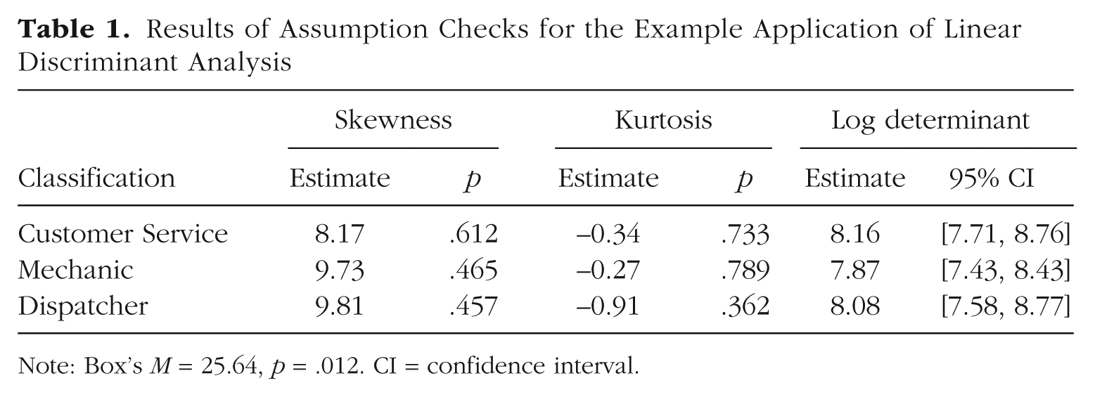
Note: Box’s M = 25.64, p = .012. CI = confidence interval.

Case classification

Running the syntax for the example produced a data set that contained the observed predictors and actual classification of cases, along with the predicted classification, the posterior probabilities, and the typicality probabilities for each case (see Table 2 for sample results).

Table 2.

Results for Six Cases in the Example Application of Linear Discriminant Analysis

Case	Predictor score			Observed job	Predicted job	Posterior probability			Typicality probability
Case	Outdoor skills	Social skills	Conservativeness	Observed job	Predicted job	Customer Service	Dispatcher	Mechanic	Customer Service	Dispatcher	Mechanic
1	10	22	5	Cust Serv	Cust Serv	.91	.01	.08	.58	.01	.08
2	14	17	6	Cust Serv	Mechanic	.37	.19	.45	.29	.16	.34
3	19	33	7	Cust Serv	Cust Serv	.75	< .01	.25	.08	< .01	.03
4	14	29	12	Cust Serv	Cust Serv	.82	.01	.17	.58	.01	.16
5	14	25	7	Cust Serv	Cust Serv	.78	< .01	.21	.91	.03	.37
16	18	25	5	Cust Serv	Cust Serv	.51	< .01	.48	.35	< .01	.33

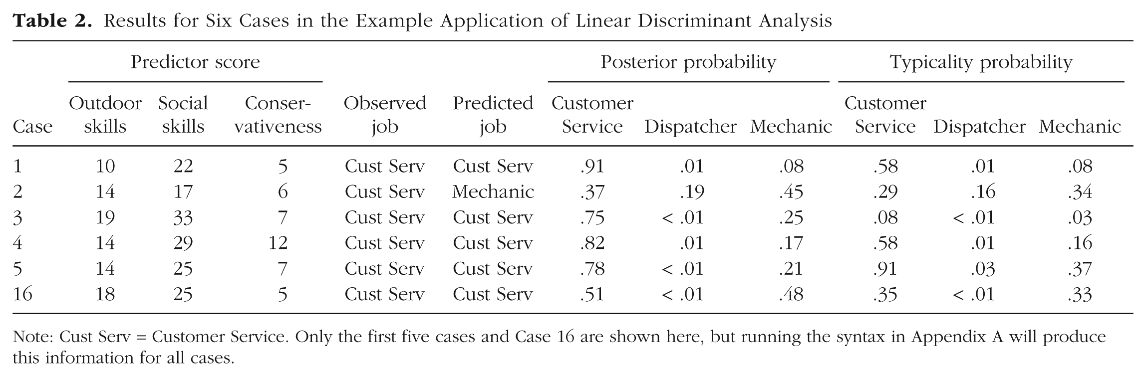
Note: Cust Serv = Customer Service. Only the first five cases and Case 16 are shown here, but running the syntax in Appendix A will produce this information for all cases.

Researchers should inspect the typicality probabilities for outliers and fence riders. Huberty and Wisenbaker (1992) suggested that a case with a typicality probability less than .10 for its assigned class should be considered an outlier. For example, in our output, Case 3 had a typicality probability of .078 for its assigned class (Table 2). Although this case was correctly classified, the inclusion of such an outlying data point can influence the coefficients of the LCFs. Huberty and Wisenbaker recommended removing such cases from the analysis, although caution should be taken in doing so because of the potential for overfitting the model or redefining the population of interest. Case 16 would be considered a fence rider, with posterior probabilities of .510 for Customer Service and .483 for Mechanic (Table 2). Because there were only a small number of outliers and fence riders in our output, we did not remove any cases.

Overall classification

After considering the potential influence of outliers and fence riders, we evaluated the overall classification of cases by examining hit rates and Huberty’s I index. Given the bias inherent to internal classification, we used CV methods to determine hit rates. The hit rates were .746 for LOO CV, .738 for k-fold CV (with k = 10), and .741 for repeated k-fold CV (with k = 10 and repetitions = 20). These hit rates should be considered in light of the chance hit rate. The chance hit rate was calculated by substituting into Equation 1 the prior probability of each occupation (e.g., .333 for each), sample size (85, 93, and 66), and total sample size (244). The chance hit rate was .333. Although the hit rates (i.e., .738–.746) appeared to be relatively large compared with a chance hit rate of .333, the final step was calculating Huberty’s I index. We used the LOO-CV hit rate in Equation 2 and found that Huberty’s I was .619.³ Huberty and Lowman (2000) suggested that an I index of .35 is a general and conservative threshold for a high (or large) effect. Thus, the I index for this example is considered a large effect.

Overall, this analysis indicates that the industrial-organizational psychologists working for the airline could conclude that the three job classifications did, in fact, appeal to different personality types. The LCFs derived from measures of outdoor skills, social skills, and conservativeness correctly classified approximately 75% of the participants in the study—a marked improvement over chance, evidenced by a large effect size.

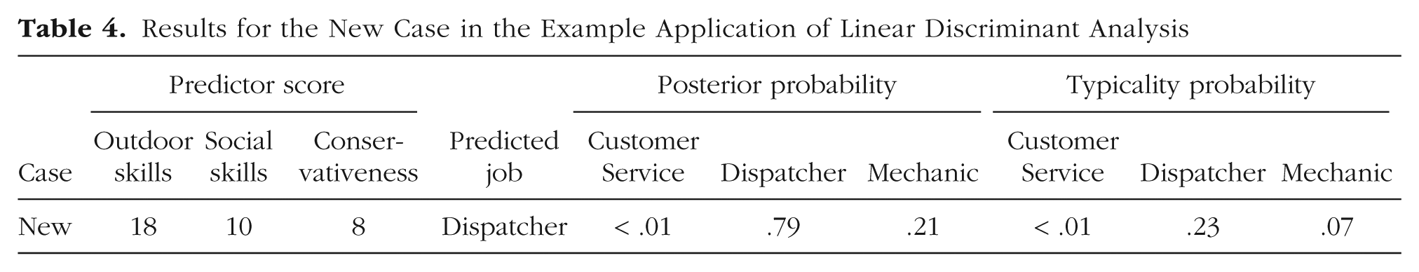
Classifying a new case

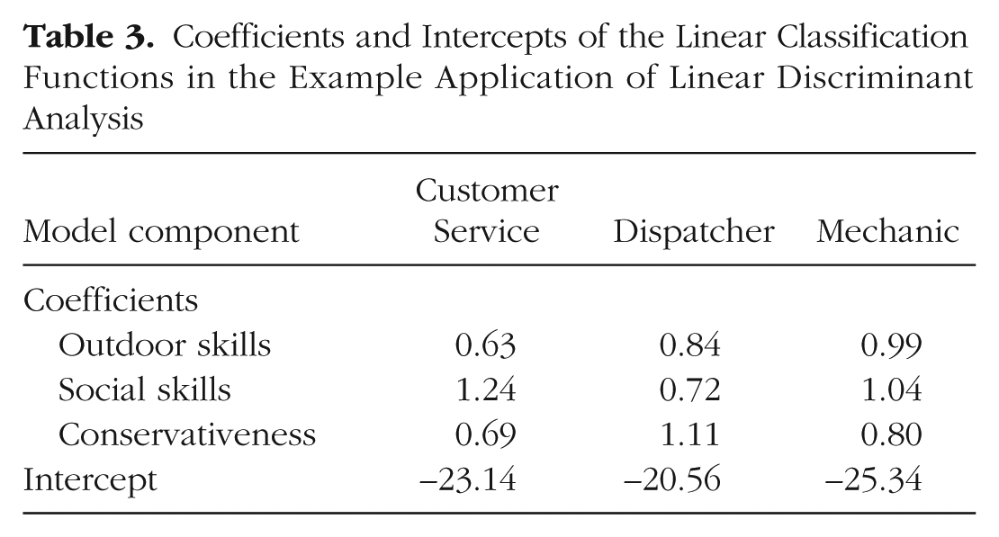
The coefficients and intercepts of the LCFs derived in the training data set, shown in Table 3, can be applied to an unclassified case to predict classification. As an example, we applied the LCFs to a case with a score of 18 for outdoor skills, a score of 10 for social skills, and a score of 8 for conservativeness, substituting these values in to the LCF for each classification. The results, including posterior probabilities and typicality probabilities, are presented in Table 4. According to the results, the new example case belongs with the Dispatcher group because of the high posterior probability and comparatively large typicality probability for that group. Psychologists working for the airline could be confident that the assignment is likely correct for this case because the cross-validated classification with the training data was favorable.

Table 3.

Coefficients and Intercepts of the Linear Classification Functions in the Example Application of Linear Discriminant Analysis

Model component	Customer Service	Dispatcher	Mechanic
Coefficients
Outdoor skills	0.63	0.84	0.99
Social skills	1.24	0.72	1.04
Conservativeness	0.69	1.11	0.80
Intercept	−23.14	−20.56	−25.34

Table 4.

Results for the New Case in the Example Application of Linear Discriminant Analysis

Case	Predictor score			Predicted job	Posterior probability			Typicality probability
Case	Outdoor skills	Social skills	Conservativeness	Predicted job	Customer Service	Dispatcher	Mechanic	Customer Service	Dispatcher	Mechanic
New	18	10	8	Dispatcher	< .01	.79	.21	< .01	.23	.07

Conclusion

This Tutorial is meant to serve as a practical and applied overview of LDA for prediction of group membership. Though several classification methods exist, LDA has been shown to operate comparatively well when the number of predictors is fewer than half the number of cases, the correlations between predictors is greater than .60, and the assumptions of the model are approximately met. LDA also may be preferred over logistic and multinomial logistic regression when specification of a reference group is inappropriate or under conditions of separability. For evaluating overall classification, repeated k-fold cross-validation is recommended, when possible, and Huberty’s I index is the recommended effect size for determining whether the classification model performs better than chance. Posterior probabilities indicate the probability of group membership, and typicality probabilities are useful for identifying outliers or pointing to a potentially unnamed class. Psychological researchers interested in a more intricate understanding of LDA should consult Huberty’s (1994) or Huberty and Olejnik’s (2006) books concerning applied discriminant analysis, as well as the works we have cited throughout this article.

Supplemental Material

Boedeker_Open_Practices_Disclosure – Supplemental material for Linear Discriminant Analysis for Prediction of Group Membership: A User-Friendly Primer

Supplemental material, Boedeker_Open_Practices_Disclosure for Linear Discriminant Analysis for Prediction of Group Membership: A User-Friendly Primer by Peter Boedeker and Nathan T. Kearns in Advances in Methods and Practices in Psychological Science

Footnotes

Appendix A: Annotated R Syntax for the Example of Linear Discriminant Analysis Discussed in the Main Text

# LDA

install.packages("lda")

install.packages("MVN")

install.packages("heplots")

install.packages("caret")

library(lda)

library(MVN)

library(heplots)

library(caret)

# Get Airline Data from UCLA website

library(haven)

AirlineData <- read_sav("https://stats.idre.ucla.edu/stat/data/discrim.sav")

View(AirlineData)

AirlineData <- as.data.frame(AirlineData)

AirlineData <- AirlineData[,-5]

# Recode JOB

# 1 = Customer Service (CS), 2 = Mechanic # (Mech), 3 = Dispatcher (Disp)

AirlineData$JOB[AirlineData$JOB==1] <- "CS"

AirlineData$JOB[AirlineData$JOB==2] <- "Mech"

AirlineData$JOB[AirlineData$JOB==3] <- "Disp"

# Number of classifications

n.class <- 3

# Select prior - in the example we use an # equal prior for each of the three groups

prior <- 1/n.class

# Number of predictors

p <- 3

# Number of cases

N <- length(AirlineData[,1])

############### Contents: ##############

# (1) Separate dataset by classification

# Assumptions

# (2) Assess multivariate normality (within # groups)

# (3) Assess equality of var-cov matrices

# Case Classification

# (4) Deriving LCFs and LCF scores [Necessary # for getting LCFs]

# (5) Posterior probability [Shown here # for completeness, "under the hood" of # lda function]

# (6) Typicality probabilities

# Evaluate overall classification # accuracy

# (7) LOO, k-fold, and repeated k-fold CV # methods

# (8) Huberty’s I-Index

# (9) Apply to a new case

########################################

# (1) Separate dataset by classification

########################################

data.CS <- subset(AirlineData, AirlineData$JOB=="CS")

data.Mech <- subset(AirlineData, AirlineData$JOB=="Mech")

data.Disp <- subset(AirlineData, AirlineData$JOB=="Disp")

########################################

# (2) Assess multivariate normality # (within groups)

########################################

mvn(data = data.CS[1:3], multivariatePlot = "qq", mvnTest = "mardia")

mvn(data = data.Mech[1:3], multivariatePlot = "qq", mvnTest = "mardia")

mvn(data = data.Disp[1:3], multivariatePlot = "qq", mvnTest = "mardia")

########################################

# (3) Assess equality of var-cov matrices

########################################

# Box’s M

hm.vc <- boxM(AirlineData[1:3], AirlineData[,"JOB"])

hm.vc

# Log-determinants and 95% CI for # log-determinants

logdetCI(cov(data.CS[1:3]), n = length(data.CS[,1]))

logdetCI(cov(data.Mech[1:3]), n = length(data.Mech[,1]))

logdetCI(cov(data.Disp[1:3]), n = length(data.Disp[,1]))

########################################

### Case Classification ###

########################################

# Run the LDA using the lda function

output <- lda(JOB ~ ., AirlineData, prior = c(prior,prior,prior))

# Get the posterior values and predicted # classification for each case

pred <- predict(output)

# Posterior values for each class for # each case

posteriors <- pred$posterior

# Predicted Class

predclass <- pred$class

# Putting Data (including actual class) # next to predicted class and posterior values

PostAirline <- cbind(AirlineData,predclass,posteriors)

colnames(PostAirline) <- c("OUTDOOR","SOCIAL","CONSERVATIVE","JOB","predclass",

"postCS","postDisp","postMech")

########################################

# (4) Deriving LCFs and LCF scores – Not # necessary for the example but here for # completeness

########################################

# (a) Means of predictors within each class

mean.CS <- c(mean(data.CS$OUTDOOR),mean(data.CS$SOCIAL),mean(data.CS$CONSERVATIVE))

mean.Mech <- c(mean(data.Mech$OUTDOOR),mean(data.Mech$SOCIAL),mean(data.Mech$CONSERVATIVE))

mean.Disp <- c(mean(data.Disp$OUTDOOR),mean(data.Disp$SOCIAL),mean(data.Disp$CONSERVATIVE))

mean.CS <- as.matrix(mean.CS)

mean.Mech <- as.matrix(mean.Mech)

mean.Disp <- as.matrix(mean.Disp)

# (b) variance-covariance matrix within # each class

cov.CS <- cov(data.CS[1:3])

cov.Mech <- cov(data.Mech[1:3])

cov.Disp <- cov(data.Disp[1:3])

# (c) sample size for each class

n.CS <- dim(data.CS)[1]

n.Mech <- dim(data.Mech)[1]

n.Disp <- dim(data.Disp)[1]

# (d) degrees of freedom used when # pooling variance-covariance matrices

# *If QDA were being used, the variance-# covariance matrices would not be pooled

cov.df <- n.CS+n.Mech+n.Disp-n.class

# (e) pooling variance-covariance matrices

cov.d <- ((n.CS-1)/cov.df)*cov.CS + ((n.Mech-1)/cov.df)*cov.Mech + ((n.Disp-1)/cov.df)*cov.Disp

# (f) determinant of the pooled # variance-covariance matrix

d <- det(cov.d)

# data to be classified (example for a # single case, not necessary for deriving LCFs)

classify <- AirlineData[1,1:3]

classify <- as.matrix(classify)

# (g) Coefficients of LCFs for # predictors within each classification

cj.CS <- solve(cov.d)%*%mean.CS

cj.Mech <- solve(cov.d)%*%mean.Mech

cj.Disp <- solve(cov.d)%*%mean.Disp

# (h) Intercept of LCFs within each # classification

cj0.CS <- -.5*t(cj.CS)%*%mean.CS

cj0.Mech <- -.5*t(cj.Mech)%*%mean.Mech

cj0.Disp <- -.5*t(cj.Disp)%*%mean.Disp

# (i) The prior adds an additional # component to the equation: log(prior) # for that class.

# In our example, the prior is equal across # classes.

p.CS <- classify%*%cj.CS + cj0.CS + log(prior)

p.Mech <- classify%*%cj.Mech + cj0.Mech + log(prior)

p.Disp <- classify%*%cj.Disp + cj0.Disp + log(prior)

########################################

# (5) Posterior probability – Not # necessary for the example but here # for completeness

########################################

# A fully Bayesian approach can be # utilized to estimate the posterior # probability of a case for every # possible classification. The same test # case is used here as an example.

fCS.1 <- (1/(((2*pi)^(p/2))*(d^.5)))*exp(-.5*(t(t(classify)-mean.CS))%*%solve(cov.d)%*%(t(classify)-mean.CS))

fDisp.1 <- (1/(((2*pi)^(p/2))*(d^.5)))*exp(-.5*(t(t(classify)-mean.Disp))%*%solve(cov.d)%*%(t(classify)-mean.Disp))

fMech.1 <- (1/(((2*pi)^(p/2))*(d^.5)))*exp(-.5*(t(t(classify)-mean.Mech))%*%solve(cov.d)%*%(t(classify)-mean.Mech))

posterior.1CS <- (fCS.1*prior)/(fCS.1*prior+fMech.1*prior+fDisp.1*prior)

posterior.1Disp <- (fDisp.1*prior)/(fCS.1*prior+fMech.1*prior+fDisp.1*prior)

posterior.1Mech <- (fMech.1*prior)/(fCS.1*prior+fMech.1*prior+fDisp.1*prior)

########################################

# (6) Typicality probabilities

########################################

# Creating a matrix for receiving # typicality results

typicality <- matrix(NA, N, n.class)

colnames(typicality) <- c("typCS","typDisp","typMech")

# The typicality is found in the right # tail of the chi-square distribution.

# Typicality can be calculated for each # case for each classification.

# df = number of variables

for (q in 1:N){

case <- matrix(NA,3,1)

case <- c(AirlineData[q,1],AirlineData[q,2],AirlineData[q,3])

d2.cs <- (t(case-mean.CS))%*%solve(cov.d)%*%(case-mean.CS)

typicality[q,1] <- pchisq(d2.cs, df = 3, lower.tail = F)

d2.disp <- (t(case-mean.Disp))%*%solve(cov.d)%*%(case-mean.Disp)

typicality[q,2] <- pchisq(d2.disp, df = 3, lower.tail = F)

d2.mech <- (t(case-mean.Mech))%*%solve(cov.d)%*%(case-mean.Mech)

typicality[q,3] <- pchisq(d2.mech, df = 3, lower.tail = F)

}

# Create a dataset with original data, # predicted classification, posterior # and typicality results

PostTypAirline <- cbind(PostAirline, typicality)

View(PostTypAirline)

########################################

### Evaluate overall classification accuracy ###

########################################

# (7) LOO, k-fold, and repeated k-fold # CV methods

########################################

# (a) LOO, done in lda when CV = T

LOO.cv <- lda(JOB ~ ., AirlineData, CV = T, prior=c(1,1,1)/3)

LOOoutcome <- table(LOO.cv$class, AirlineData$JOB)

# Prediction accuracy:

LOOhitrate <- (LOOoutcome[1,1]+LOOoutcome[2,2]+LOOoutcome[3,3])/N

# (b) k-fold cross-validation

train_control <- trainControl(method="cv", number=10, savePredictions = TRUE, classProbs = TRUE)

k.cv <- train(JOB ~ ., data=AirlineData, trControl=train_control, method="lda", prior=c(1,1,1)/3)

koutcome <- table(k.cv$pred$pred, k.cv$pred$obs)

# Prediction accuracy:

khitrate <- (koutcome[1,1]+koutcome[2,2]+koutcome[3,3])/N

# (c) Repeated k-fold cross-validation

# m.cv = number of iterations of k-fold # cross validation

# kfold = number of groups

# data = full data set to be split

m.cv <- 20

kfold <- 10

repkfinaloutcome <- matrix(NA, m.cv, 1)

for (t in 1:m.cv){

train_control<- trainControl(method="cv", number=kfold, savePredictions = TRUE, classProbs = TRUE)

model<- train(JOB ~ ., data=AirlineData, trControl=train_control, method="lda", prior=c(1,1,1)/3)

repkoutcome <- table(model$pred$pred, model$pred$obs)

# Prediction accuracy:

repkfinaloutcome[t,] <- (repkoutcome[1,1]+repkoutcome[2,2]+repkoutcome[3,3])/N

}

repkhitrate <- mean(repkfinaloutcome)

########################################

# (8) Huberty’s I-Index

########################################

# If using LOO CV with repeated # iterations

Ho <- LOOhitrate

#Ho <- khitrate

#Ho <- repkhitrate

Hc <- (prior*length(data.CS[,1])+prior*length(data.Mech[,1])+prior*length(data.Disp[,1]))/N

Huberty.I <- (Ho-Hc)/(1-Hc)

########################################

# (9) Apply to a new case

########################################

# Using the LCFs derived in (2), we can # classify a case based on the observed

# variables of that case.

# Example, if we are classifying the # case with

# OUTDOOR = 18

# SOCIAL = 10

# CONSERVATIVE = 8

new.case <- c(18, 10, 8)

# (a) To get classification score

p.CS <- new.case%*%cj.CS + cj0.CS + log(prior)

p.Mech <- new.case%*%cj.Mech + cj0.Mech + log(prior)

p.Disp <- new.case%*%cj.Disp + cj0.Disp + log(prior)

# (b) Posterior Probability

#CS

post.CS <- (exp(p.CS-p.CS))/(exp(p.Mech-p.CS)+exp(p.CS-p.CS)+exp(p.Disp-p.CS))

#Mech

post.Mech <- (exp(p.Mech-p.CS))/(exp(p.Mech-p.CS)+exp(p.CS-p.CS)+exp(p.Disp-p.CS))

#Disp

post.Disp <- (exp(p.Disp-p.CS))/(exp(p.Mech-p.CS)+exp(p.CS-p.CS)+exp(p.Disp-p.CS))

# (c) Typicality probability

d2.cs <- (t(new.case-mean.CS))%*%solve(cov.d)%*%(new.case-mean.CS)

typ.cs <- pchisq(d2.cs, df = p, lower.tail = F)

d2.mech <- (t(new.case-mean.Mech))%*%solve(cov.d)%*%(new.case-mean.Mech)

typ.mech <- pchisq(d2.mech, df = p, lower.tail = F)

d2.disp <- (t(new.case-mean.Disp))%*%solve(cov.d)%*%(new.case-mean.Disp)

typ.disp <- pchisq(d2.disp, df = p, lower.tail = F)

# Automated process of classifying a new # dataset using the lda package

new.data <- data.frame(‘OUTDOOR’ = c(18,13,9), ‘SOCIAL’ = c(10,20,31), ‘CONSERVATIVE’ = c(8,5,9))

# output is from original run of lda # under “Case Classification” section

predict(output, new.data)

Appendix B: Derivation of Linear Classification Functions and Bayesian Posterior Probabilities

This appendix provides technical details regarding the derivation of linear classification functions (LCFs) in a Bayesian framework. The LCFs output a classification score for each group for a given case, and these scores can be used to derive the posterior probabilities of group membership.

The posterior probability is the probability that an individual with response vector x for the set of predictors X is a member of group k out of the possible set of groups G. To estimate this probability, we utilize Bayes theorem:

(B1)

P r (G = k | X = x) = \frac{P r (X = x | G = k) P r (G = k)}{\sum_{j = 1}^{k} P r (X = x | G = j) P r (G = j)},

where Pr(X = x|G = k) is the likelihood of observing the response vector given membership in group k, Pr(G = k) is the prior probability of membership in group k, and $\sum_{j = 1}^{k} P r (X = x | G = j) P r (G = j)$ is the sum of all products of prior probabilities and likelihood given a response vector over the possible classifications. The result, Pr(G = k|X = x), is the posterior probability of membership in k given a case’s response vector for the predictors X.

Assuming a multivariate normal distribution of predictors, the density of the predictors within a class k is estimated as follows:

f_{k} (x) = \frac{1}{{(2 π)}^{\frac{p}{2}} {| \sum |}^{\frac{1}{2}}} e^{- \frac{1}{2} {(x - μ_{k})}^{T} Σ^{- 1} (x - μ_{k})},

where p is the number of predictors, and T indicates transposition. This estimate is equivalent to Pr(X = x|G = k) in Equation B1. The term ${(x - μ_{k})}^{T} Σ^{- 1} (x - μ_{k})$ is a case’s Mahalanobis distance from the kth centroid; the Σ is the pooled within-class variance-covariance matrix. Note also that the denominator in Equation B1 is the same regardless of the class k for a given response vector, and thus can be written as a single constant, C. If we simplify terms by writing the prior probability of class k as π_k, Equation B1 can be written as

P r (G = k | X = x) = \frac{C π_{k}}{{(2 π)}^{\frac{p}{2}} {| Σ |}^{\frac{1}{2}}} e^{- \frac{1}{2} {(x - μ_{k})}^{T} Σ^{- 1} (x - μ_{k})} .

Every term that does not depend on k will remain constant and can be written as a single constant, C′, such that

P r (G = k | X = x) = C^{'} π_{k} e^{- \frac{1}{2} {(x - μ_{k})}^{T} Σ^{- 1} (x - μ_{k})} .

To maximize over k groups, we first take the log:

\begin{array}{l} l o g P r (G = k | X = x) = l o g C' + \\ l o g π_{k} - \frac{1}{2} {(x - μ_{k})}^{T} Σ^{- 1} (x - μ_{k}) . \end{array}

We note that log C′ does not vary by k. Therefore, to determine classification, we maximize only the variable terms over the k groups:

l o g π_{k} - \frac{1}{2} {(x - μ_{k})}^{T} Σ^{- 1} (x - μ_{k}) .

Expanding this final term and simplifying yields

l o g π_{k} - \frac{1}{2} x^{T} Σ^{- 1} x - \frac{1}{2} μ_{k}^{T} Σ^{- 1} μ_{k} + x^{T} Σ^{- 1} μ_{k} .

However, the second term in this expression also does not depend on k. Therefore, to find the maximum over the k possible classes, we need only use the following:

(B2)

l o g π_{k} - \frac{1}{2} μ_{k}^{T} Σ^{- 1} μ_{k} + x^{T} Σ^{- 1} μ_{k} .

The first term in Equation B2 is dependent entirely on the prior probability of membership in group k. The second term is a constant dependent on the mean of the predictor variables, or centroid, within group k. The sum of the first and second terms yields the LCF’s intercept for the kth group. The final term is the product of a case’s vector of observed responses to predictor variables and the coefficients of the LCF for the kth group. Substituting a single case’s response vector into Equation B2 produces a classification score from which the posterior probability of group membership may also be derived.

Action Editor

Frederick L. Oswald served as action editor for this article.

Author Contributions

N. T. Kearns wrote an initial draft of the manuscript. P. Boedeker substantially revised the manuscript and wrote the syntax for the data analysis. Both authors critically edited the manuscript and approved the final submitted version.

ORCID iDs

Peter Boedeker

Nathan T. Kearns

Declaration of Conflicting Interests

The author(s) declared that there were no conflicts of interest with respect to the authorship or the publication of this article.

Open Practices

Open Data: not applicable

Open Materials:

Preregistration: not applicable

All materials have been made publicly available via the Open Science Framework and can be accessed at https://osf.io/6bk24/files/. The complete Open Practices Disclosure for this article can be found at http://journals.sagepub.com/doi/suppl/10.1177/2515245919849378. This article has received the badge for Open Materials. More information about the Open Practices badges can be found at .

Notes

References

Boedeker

(2017). Hierarchical linear modeling with maximum likelihood, restricted maximum likelihood, and fully Bayesian estimation. Practical Assessment, Research and Evaluation, 22, 1–19.

Box

G. E. P.

(1949). A general distribution theory for a class of likelihood criteria. Biometrika, 36, 317–346.

Braga-Neto

U. M.

Dougherty

E. R.

(2004). Is cross-validation valid for small-sample microarray classification? Bioinformatics, 20, 374–380. doi:10.1093/bioinformatics/btg419

Brown

Mues

(2012). An experimental comparison of classification algorithms for imbalanced credit scoring data sets. Expert Systems With Applications, 39, 3446–3453. doi:10.1016/j.eswa.2011.09.033

Cai

T. T.

Liang

Zhou

H. H.

(2015). Law of log determinant of sample covariance matrix and optimal estimation of differential entropy for high-dimensional Gaussian distributions. Journal of Multivariate Analysis, 137, 161–172. doi:10.1016/j.jmva.2015.02.003

Enders

C. K.

(2003). Performing multivariate group comparisons following a statistically significant MANOVA. Measurement and Evaluation in Counseling and Develop-ment, 36, 40–56.

Fisher

R. A.

(1936). The use of multiple measurements in taxonomic problems. Annals of Eugenics, 7, 179–188. doi:10.1111/j.1469-1809.1936.tb02137.x

Hastie

Tibshirani

Friedman

(2009). Elements of statistical learning. New York, NY: Springer.

Henson

R. K.

(1999). Multivariate normality: What is it and how is it assessed? In Thompson

(Ed.), Advances in so-cial science methodology (Vol. 5, pp. 193–211). Stamford, CT: JAI Press.

10.

Henson

R. K.

(2002, April). The logic and interpretation of structure coefficients in multivariate general linear model analysis. Paper presented at the annual meeting of the American Educational Research Association, New Orleans, LA.

11.

Hsu

L. M.

(1989). Discriminant analysis: A comment. Journal of Counseling Psychology, 36, 244–247.

12.

Huberty

C. J.

(1994). Applied discriminant analysis (Wiley Series in Probability and Statistics Vol. 297). New York, NY: Wiley-Interscience.

13.

Huberty

C. J.

Barton

R. M.

(1989). An introduction to discriminant analysis. Measurement and Evaluation in Counseling and Development, 22, 158–168.

14.

Huberty

C. J.

Curry

A. R.

(1978). Linear versus quadratic multivariate classification. Multivariate Behavioral Research, 13, 237–245.

15.

Huberty

C. J.

Hussein

M. H.

(2003). Some problems in reporting use of discriminant analysis. The Journal of Experimental Education, 7, 177–191. doi:10.1080/00220970309602062

16.

Huberty

C. J.

Lowman

L. L.

(2000). Group overlap as a basis for effect size. Educational and Psychological Measurement, 60, 543–563.

17.

Huberty

C. J.

Olejnik

(2006). Applied MANOVA and discriminant analysis (2nd ed.). Hoboken, NJ: John Wiley & Sons.

18.

Huberty

C. J.

Wisenbaker

J. M.

(1992). Discriminant analysis: Potential improvements in typical practice. Advances in Social Science Methodology, 2, 169–208.

19.

Joachimsthaler

E. A.

Stam

(1988). Four approaches to the classification problem in discriminant analysis: An experimental study. Decision Sciences, 19, 322–333.

20.

Johnson

R. A.

Wichern

D. W.

(2007). Applied multivariate statistical analysis. Upper Saddle River, NJ: Pearson.

21.

Kessler

R. C.

Chiu

W. T.

Demler

Merikangas

K. R.

Walters

E. E.

(2005). Prevalence, severity, and comorbidity of 12-month DSM-IV disorders in the National Comorbidity Survey Replication. Archives of General Psychiatry, 62, 617–627.

22.

Khondoker

Dobson

Skirrow

Simmons

Stahl

(2016). A comparison of machine learning methods for classification using simulation with multiple real data examples from mental health studies. Statistical Methods in Medical Research, 25, 1804–1823. doi:10.1177/0962280213502437

23.

Klecka

W. R.

(1980). Discriminant analysis. Quantitative applications in the social sciences. Newbury Park, CA: Sage.

24.

Kruschke

(2013). Bayesian estimation supersedes the t test. Journal of Experimental Psychology: General, 142, 573–603. doi:10.1037/a0029146

25.

Kruschke

Aguinis

Joo

(2012). The time has come: Bayesian methods for data analysis in the organizational sciences. Organizational Research Methods, 15, 722–752. doi:10.1177/1094428112457829

26.

Lachenbruch

P. A.

(1975). Zero-mean difference discrimination and the absolute linear discriminant function. Biometrika, 62, 397–401.

27.

Lachenbruch

P. A.

Mickey

M. R.

(1968). Estimation of error rates in discriminant analysis. Technometrics, 10, 1–11.

28.

Mardia

K. V.

(1970). Measures of multivariate skewness and kurtosis with applications. Biometrika, 57, 519–530.

29.

Mardia

K. V.

(1974). Applications of some measures of multivariate skewness and kurtosis for testing normality and robustness studies. Sankhya: The Indian Journal of Statistics, Series B, 36, 115–128.

30.

R Core Team. (2018). R: A language and environment for statistical computing. Vienna, Austria: R Foundation for Statistical Computing.

31.

Rodriguez

J. D.

Perez

Lozano

J. A.

(2010). Sensitivity analysis of k-fold cross validation in prediction error estimation. IEEE Transactions on Pattern Analysis and Machine Intelligence, 32, 569–575. doi:10.1109/TPAMI.2009.187

32.

Sherry

(2006). Discriminant analysis in counseling psychology research. The Counseling Psychologist, 34, 661–683. doi:10.1177/0011000006287103

33.

Tabachnick

B. G.

Fidell

L. S.

(2013). Using multivariate statistics (3rd ed.). New York, NY: HarperCollins.

34.

UCLA Institute for Digital Research and Education. (2017). Discrim.sav [Data file]. Retrieved from https://stats.idre.ucla.edu/wp-content/uploads/2016/02/discrim.sav

35.

Warne

R. T.

(2014). A primer on multivariate analysis of vari-ance (MANOVA) for behavioral scientists. Practical Assessment, Research, & Evaluation, 19, Article 17. Retrieved from https://pareonline.net/getvn.asp?v=19&n=17

36.

Welch

B. L.

(1939). Note on discriminant functions. Biometrika, 31, 218–220.

Supplementary Material

Please find the following supplemental material available below.

For Open Access articles published under a Creative Commons License, all supplemental material carries the same license as the article it is associated with.

For non-Open Access articles published, all supplemental material carries a non-exclusive license, and permission requests for re-use of supplemental material or any part of supplemental material shall be sent directly to the copyright owner as specified in the copyright notice associated with the article.

0.00 MB

0.07 MB