Sage Journals: Discover world-class research

Abstract

Statistical prediction models are ubiquitous in psychological research and practice. Increasingly, machine-learning models are used. Quantifying the uncertainty of such predictions is rarely considered, partly because prediction intervals are not defined for many of the algorithms used. However, generating and reporting prediction models without information on the uncertainty of the predictions carries the risk of overinterpreting their accuracy. Conventional methods for prediction intervals (e.g., those defined for ordinary least squares regression) are sensitive to violations of several distributional assumptions. In this tutorial, we introduce conformal prediction, a model-agnostic, distribution-free method for generating prediction intervals with guaranteed marginal coverage, to psychological research. We start by introducing the basic rationale of prediction intervals using a motivating example. Then, we proceed to conformal prediction, which is illustrated in three increasingly complex examples using publicly available data and R code.

Keywords

tutorial machine learning prediction uncertainty open materials

Prediction is a major task of applied psychologists. Decisions about college admissions, job candidates, or the best treatment option for a particular patient all involve predictions. In most cases, the information of several variables is combined for such predictions. For example, industrial-and-organizational psychologists might want to predict job performance based on an applicant’s general mental ability and an integrity test. Psychologists can combine information from these two variables and might assign weights to them based on their judgment. Often, psychologists use statistical models based on empirical data to predict important outcomes. Decades of research have convincingly demonstrated that on average, statistical models produce more accurate predictions than humans combining the same data (Ægisdóttir et al., 2006; Meehl, 1954).

Uncertainty in Predictions

Costs and benefits are associated with the accuracy of predictions. A company that has commissioned the psychologist to select the best possible candidates is interested in ensuring that this selection is as accurate as possible. Selecting a candidate who is not right for the job means financial damage to the company. This is also the case in other fields: A forensic psychologist who predicts a low probability of reoffending for a prisoner is aware of the high costs involved if it does occur. At the same time, imprisonment is associated with high social costs if unnecessary. A clinical psychologist who intends to predict the outcomes of several different treatment options for her patients risks the continued suffering of her patients if her predictions are inaccurate. Uncertainty is inherent in all these predictions for numerous reasons. A distinction is often made between two types of uncertainty. Aleatoric uncertainty arises from the inherent unpredictability of an outcome (e.g., a dice roll). For predicting complex systems, such as human behavior, the outcome is influenced by many factors, leading to a large degree of inherent randomness. Epistemic uncertainty, on the other hand, arises from the incomplete understanding of the outcome. The model used for prediction is trained on a random, finite sample of the data. Using a different sample would result in a (slightly) different model and different predictions. In the social sciences, the predictors used for these models are often affected by measurement error, and some potentially relevant predictors are unobserved. Because of the often high degrees of aleatoric and epistemic uncertainty, it is not a question of whether the uncertainty of predictions is quantified but how it is done.

Quantifying uncertainty using prediction intervals

We now use a simple example based on simulated data to demonstrate how the uncertainty of predictions can be quantified with prediction intervals (PIs) and return to the example of the psychologist who selects applicants based on IQ and integrity tests. We assume she has access to a data set of previous applicants for which IQ test scores (M = 100, SD = 15), integrity test scores, and a job-performance rating made after 1 year by supervisors (both Ms = 50, SDs = 10). She fits an ordinary-least-squares (OLS) model predicting job performance from the other two scores, resulting in the coefficients reported in Table 1.

Table 1.

Example Regression Model Predicting Job Performance From IQ and Integrity Test Scores

Predictor	b	b [95% CI]	β	β[95% CI]	r	Fit
(Intercept)	−13.70**	[−16.88, −10.51]
IQ	0.41**	[0.39, 0.44]	0.61	[0.57, 0.65]	.64**
Integrity	0.45**	[0.41, 0.49]	0.45	[0.41, 0.49]	.49**
						R² = .612**
						95% CI = [.58, .64]

Note: b represents unstandardized regression weights. β indicates the standardized regression weights. r represents the zero-order correlation. CI = confidence interval.

p < .01.

Using this model, she can now predict the job performance of new applicants from whom she has both IQ and integrity test scores. Imagine that an applicant has an IQ of 120 and an integrity score of 40. The point prediction for this person’s job performance can be calculated as follows:

J o b \hat{P e r f o r m a n c e} = - 13.70 + 0.41 \times 120 + 0.45 \times 40 = 53.50 .

From point predictions to PIs

The values for the predictors are passed to the model, and a single value is output that represents the prediction. However, point predictions do not come with a guarantee of perfect accuracy. It is therefore advisable to quantify the uncertainty of predictions, which results in a range of values that contains the predicted value with a certain probability. Some methods for quantifying uncertainty are widespread in psychology: For estimating a population parameter, such as the mean, the sample estimate is often given a confidence interval (CI). Following a probabilistic interpretation of CIs, it can be expected with a certain probability that the population parameter lies within this interval (Schweder & Hjort, 2016; Vos & Holbert, 2022). However, when predicting future outcomes of a single observation—such as an individual’s future job performance given the person’s IQ and integrity—a PI is the appropriate method to quantify uncertainty. PIs provide a range in which a single future observation will likely fall within a certain, prespecified probability. For OLS models, the following formula gives a distributional approximation:

\hat{y} \pm t \times S E,

where $\hat{y}$ is the point prediction, t is a critical value on the t distribution (e.g., 1.96 for 95% intervals), and SE is the standard error for the PI, which is obtained as follows:

S E = s_{ϵ} \sqrt{1 + \frac{1}{n} + \frac{{(x^{*} - \bar{x})}^{2}}{(n - 1) s_{x}^{2}}},

where $s_{ϵ}$ is the standard deviation of the residuals, n is the sample size, x^* represents all values of x, and $\bar{x}$ is the sample mean of x. The psychologist could now use this formula to supplement her point prediction with a 95% PI, which, in our example, ranges from 41.94 to 66.50. This interval means that with a 95% probability, the true value for this candidate’s (unrealized) job performance will be inside this interval. A 95% CI, on the other hand, has a different interpretation: It would indicate the range in which the average job performance for individuals with an IQ of 120 and an integrity score of 40 is likely to fall. It will be much narrower than the PI (in this case, 95% CI = [53.69, 54.75]).

Note that aleatoric and epistemic uncertainty contribute to the width of a PI. As discussed, the former reflects irreducible uncertainty that is inherent in the system that is to be predicted, even with a perfect model. The latter reflects sampling variability in estimating model parameters and other imperfections. Unlike CIs, which reflect epistemic uncertainty only about a population parameter (e.g., a mean), PIs incorporate both components to capture the expected spread of future observations.

As with CIs, the width of PIs can be freely selected. The most important trade-off that needs to be considered here is between the range of predicted values covered and the informativeness of the intervals. A wider interval contains the value to be predicted with a higher probability but is also less informative. With a 95% PI, the psychologist can be very certain that the true predicted value is in this interval, but the interval spans more than 2.5 SD of the outcome variable. A greater level of uncertainty might still be acceptable. In our example, an 80% PI would range from only 45.63 to 62.10, almost 1 SD narrower.

From PIs to decisions

Decision theoretic frameworks (e.g., Liu et al., 2023) stress that outcome predictions must be judged by the impact of the decisions they imply. The psychologist in our example is tasked with selecting the best applicants based on a predictive model. Assume that the position to be filled is a highly responsible position and that the company stipulates that the position to be filled should have a job performance rating of at least 50. A straightforward strategy might be to set a threshold on the point predictions, for example, by inviting only applicants with a predicted job performance of at least 50. In the simulated example data, 84% of applicants with a point prediction of at least 50 ultimately had a true job performance rating of 50 or higher. Although this seems reasonably accurate, it means that more than one out of 10 applicants would fail to meet the performance threshold. Using PIs, the psychologist could use a three-way decision framework. She could invite the applicant if the lower bound of the PI is at least 50, and she would reject an applicant with an upper PI bound of less than 50. For the remaining cases, she would abstain from deciding and perhaps suggest these candidates for future vacancies, which can also be filled with lower performance ratings. This strategy can lead to more favorable results than using the point prediction, especially if a candidate without sufficient competence could cause great damage to the company, a suitable candidate would imply a great advantage for the company, or both. The costs and risks of these three possible decisions must ultimately be assessed according to substantive and context-specific considerations. For example, the width of the intervals can be chosen so that a certain proportion of false-positive and false-negative decisions is tolerated, which reduces the number of indecisive cases.

Challenges With Traditional Methods

So far, we have considered a relatively simple case: a linear model. As shown previously, PIs based on the normal distribution are available for these models. PIs computed this way rely on specific assumptions about the underlying distribution and assume a correctly specified model, which is hard to verify and frequently violated. If interaction effects are included, linear interactions are also assumed. Although other functional forms can be specified, these must also match the data-generating process to ensure correct PIs. Second, other assumptions of the linear model, such as normally distributed residuals with a constant variance across all levels of the predictors, need to be met. Each observation is assumed to be drawn independently of others from the same underlying distribution. The coverage probability—the likelihood that the PI contains the true value—may not align with the nominal level (e.g., 95%) when these assumptions are violated. This discrepancy can lead to misinformed decisions, such as overestimating the suitability of a job candidate or underestimating the risk of a negative clinical outcome.

As Yarkoni and Westfall (2017) argued, prediction is often the primary goal in many applied psychological disciplines. However, methods such as linear regression, although frequently used in psychology to explain data, might not be the best choice for generating the most accurate predictions. Machine-learning algorithms enable researchers to relax some assumptions that need to be held when using OLS. For example, penalized regression methods (e.g., ridge, least absolute shrinkage and selection operator [LASSO], or elastic net regression [ENR]) help generate more generalizable predictive models. Decision-tree-based methods, such as random forests, are often helpful for dealing with complex data patterns because they do not assume specific functional forms. Unlike OLS, however, most of these methods lack straightforward approaches to uncertainty quantification.

Alternative Methods for PIs

In addition to OLS-based intervals, more elaborate methods have been proposed for generating PIs. For example, PIs can be generated by bootstrapping procedures. Here, the data are repeatedly sampled with replacement from the data, resulting in a distribution of predictions. The percentiles of this distribution can be taken as a PI. Bayesian approaches can be used to model the conditional distribution (i.e., the conditional mean) to obtain a full posterior predictive distribution, from which PIs can also be constructed. Like the OLS approach, these intervals make distributional assumptions. In the case of Bayesian statistics, the assumption is that the distribution of priors and the selected distribution family match the data-generating process. If this is not the case, the nominal coverage value will not correspond to the actual coverage.

Ensemble-based methods, such as deep ensembles (Lakshminarayanan et al., 2017) or random forests (Breiman, 2001), estimate uncertainty by aggregating predictions from multiple models. In the random forest, PIs can be obtained by aggregating many decision trees on separate subsets of the original data and leaving out a smaller subset for validation; “out-of-bag” uncertainty estimates can be obtained from the prediction errors of the validation data set. Another major approach is the direct estimation of conditional quantiles. These approaches do not model a distribution but use a loss function that is constructed for using it with PIs. This approach includes quantile regression (Koenker & Hallock, 2001), which is an extension of OLS regression that estimates conditional quantiles, but also more complex algorithms based on random forests (called “quantile forests”) or neural networks. Although providing an in-depth overview on different approaches to quantifying predictive uncertainty is beyond the scope of this tutorial, we refer the reader to a recent review by Dewolf et al. (2023), which discusses many newer, machine-learning-based approaches as well.

Conformal Prediction

Conformal prediction (Lei & Wasserman, 2014; Papadopoulos et al., 2002; Vovk et al., 2005) is a versatile framework for quantifying the uncertainty of any predictive model. It is distribution-free such that it makes no assumptions about the distribution of the data. It is also model-agnostic, meaning it can be applied to any predictive model and independently of the task of the model. This also includes direct estimation procedures, such as quantile regression.

General approach

Conformal-prediction algorithms generally follow the same three steps: training, calibration, and prediction. During training, the data are split into a training data set and a calibration data set. Algorithms differ in how exactly the splitting is done. In the simplest case, a certain, larger portion of the data is used as training set, and a smaller portion is used for calibration. This would require splitting the data and fitting the model only once. Other approaches split the data several times and refit the model in each step. This procedure, called “cross-conformal prediction,” is computationally more intensive but sometimes produces smaller PIs.

The statistical model is fit to the training data and then used to predict the (unseen) values in the calibration data set. In the calibration step, predicted values are compared with true values, and based on how strongly they differ, uncertainty scores (also referred to as “nonconformity scores”) are computed. These scores are measures for the inaccuracy of predictions. The higher a nonconformity score is, the more inaccurate was a prediction. The scores are then sorted in increasing order. The user decides on a confidence level (a). For example, an a of .10 means that on average, 90% PIs generated will include the true value. The quantile of 1 – a (90th percentile if a = .10) of the nonconformity scores is determined. This value is commonly referred to as the “threshold.” In the prediction step, the model is used for predicting new data. For predicting continuous outcomes (i.e., regression), the threshold is added to the predicted value to obtain the upper bound of the PI and subtracted to obtain the lower bound.

Marginal and conditional coverage

Sets of PIs generated with conformal prediction come with a mathematically proven guaranteed marginal coverage. This means that the prespecified nominal coverage rate (e.g., 90%) will be guaranteed to be met, on average (i.e., 90% of PIs contain the true value), for samples from the distribution of the calibration or test data.

Conformal prediction is the only approach to provide this guarantee. As noted by Cabezas et al. (2025), other methods “fail to provide even marginally valid predictive intervals in the finite-sample setting.” Marginal coverage is very useful for evaluating how well a predictive model performs in general. If it is guaranteed, models can be compared based on the width of their PIs. Without such a guarantee, it cannot be ruled out that differences in the width of the intervals are due to violated model assumptions and misspecification.

Conformal prediction does not guarantee conditional coverage. This would mean that the model guarantees the desired coverage rate not only on average but also given specific values of covariates in the model. For example, a researcher might have obtained a data set that contains half men and half women. Even if the researcher specified a 90% certainty level, the outcome of women might be harder to predict (possibly because of unobserved variables, a lack of measurement invariance of the measures used, etc.), leading to an actual coverage rate of 80% for women. The outcomes of men could be predicted more accurately (100% coverage). The conformal PIs generated for this data set will still reach a marginal coverage of 90%, but conditional coverage would be achieved if the coverage rate is 90% for both men and women. The model would have to adjust the width of its PIs, depending on whether it is predicting for a man or a woman. This implies an interpretational leap from marginal coverage to individual certainty: They cannot be interpreted as providing 90% certainty for any given individual.

It is an important advantage of distribution-based approaches that they offer some degree of guaranteed conditional coverage. For example, if model assumptions are met, PIs generated from an OLS model using the distributional formula guarantee conditional coverage in very large samples (asymptotic conditional coverage). Under the assumption that the model and all prior distributions are correctly specified, Bayesian methods provide approximate conditional coverage in finite samples as well. For deciding on a method for generating PIs, the decision therefore plays a role as to whether to rely on the most complete possible fulfillment of the model assumptions or to accept certain limitations in the conditional coverage.

On the other hand, although conditional coverage cannot be guaranteed by any distribution-free approach (Lei & Wasserman, 2014), extensions of conformal prediction were developed to mitigate this problem (Angelopoulos & Bates, 2022). These methods work by adapting the width of the PIs depending on the characteristics of the covariates. They are appealing because the desirable properties of conformal PIs are preserved, and the conditional coverage approaches that of other methods under real-world conditions. We provide an example for such a method in the third example.

Assumptions

Conformal prediction guarantees finite-sample marginal coverage of 1 – α, under the assumption of exchangeability. This means that across all possible permutations of calibration and test points, the PI will contain the true outcome with the desired probability. Although exchangeability is a weaker assumption than those made by many parametric methods, it is not assumption-free, and there are cases in which exchangeability is violated. When using conformal prediction for time-series data, which often shows trends and cycles, one can no longer assume exchangeability. Violations of this assumption can also happen because of distributional shift between calibration and test data sets, for example, when predicting for a demographically different data set or when the test data were sampled differently compared with the training sample. In such cases, conformal PIs may no longer achieve valid marginal coverage, and the nominal coverage rate may be overachieved or underachieved. Although in this tutorial, we focus on settings in which exchangeability is plausible, methods have been developed to relax this assumption, including conformal prediction for time series (Xu & Xie, 2021), which were shown to provide approximate marginal coverage. Weighted conformal prediction (Tibshirani et al., 2019) addresses covariate shift by modifying the exchangeability assumption.

Beyond the formal statistical assumption of exchangeability, some practical requirements need to be considered so that useful PIs can be generated. The nonconformity scores must match the prediction task (regression, classification), reflect the prediction inaccuracy, and thus be ordered in such a way that the smallest score reflects the most accurate prediction. In addition, there must be sufficient data for calibration, which we discuss in the next section.

Sample size

The sample size of the training data set will influence how precisely the parameters of the respective statistical model can be estimated. This will lead to more or less accurate predictions and, therefore, smaller or larger nonconformity scores. Although this does not affect the marginal coverage guarantee of the intervals, which is always maintained, the size of the calibration data set is an additional factor in conformal prediction that needs to be considered. As Angelopoulos and Bates (2022) noted, the coverage guarantee in general holds for calibration sets of any size, but conditional on any fixed calibration data set, coverage will fluctuate somewhat. As a consequence, the observed coverage observed when using small data sets might deviate from the chosen certainty level. In psychology, measures with relatively coarse-grained scales, such as Likert or visual-analog scales, are often used. This makes it more likely that residuals or predicted probabilities will repeat across cases, resulting in ties that further contribute to these deviations. The resulting fluctuation around the chosen certainty level is called “coverage slack” (Angelopoulos & Bates, 2022, p. 14). For a summary of coverage-slack values that can be expected based on a range of sample sizes and a certainty level of 90%, including the expected range of marginal coverage, see Table 2. Note that this does not affect the finite-sample marginal coverage guarantee but is a consequence of the practical implementation of conformal prediction using a given calibration data set. We provide an R function to compute the coverage slack for any given N in the supplement (https://osf.io/d9w8n/; file: compute_coverage_slack.R).

Table 2.

Coverage Slack and Corresponding Coverage Ranges for Some Calibration-Set Sample Sizes

Sample size	50	100	250	500	1,000
Coverage slack	0.09	0.06	0.04	0.03	0.02
95% coverage range	0.81–0.99	0.84–0.96	0.86–0.94	0.87–0.93	0.88–0.92

Note: The 95% coverage range indicates that the marginal coverage obtained from a single calibration set of the given size is within this range with a probability of 95% using an infinite test data set.

Comparison with standard methods

Traditional methods for constructing PIs—such as those based on normality assumptions, mean-variance estimation, or ensemble uncertainty—often fail to provide valid coverage in finite samples or under model misspecification. Dewolf (2024) systematically compared a range of PI methods across multiple data sets, including neural networks, random forests, quantile regressors, deep ensembles, and Gaussian processes. The study demonstrated that other methods frequently produced intervals with either coverage below the nominal level or excessive width. In contrast, conformalized versions of these models consistently achieved the prespecified nominal marginal coverage, with intervals that were often narrower or equally efficient compared with other methods. Because conformal prediction can be combined with any model, we also compared how PIs of a method using the full data compare with conformal PIs. Here, too, we found that the conformal PIs were significantly closer to the desired coverage rate.

In the first example, we introduce the general procedure of this approach using OLS regression.

Example 1: general procedure

As introduced previously, quantifying uncertainty using conformal prediction follows some general steps (Angelopoulos & Bates, 2023) that we demonstrate using the previous example of job-candidate selection. R code to reproduce all the following examples is available at https://osf.io/d9w8n/ (file: EX1_job_performance.R). For the necessary code to perform the steps described in this example, see Table 3.

Table 3.

Full R Code for Example 1 (Ordinary Least Squares + Prediction Interval)

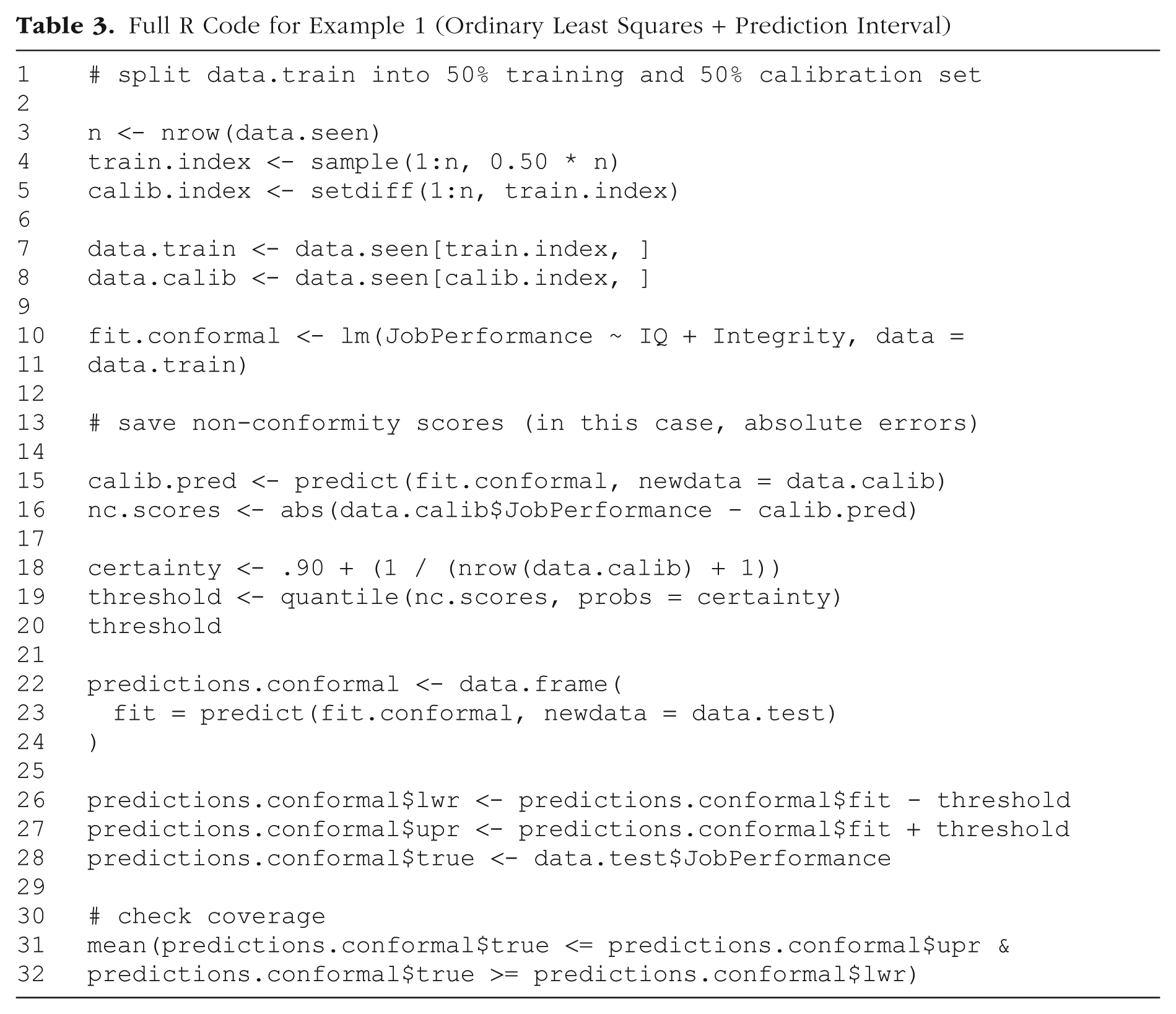
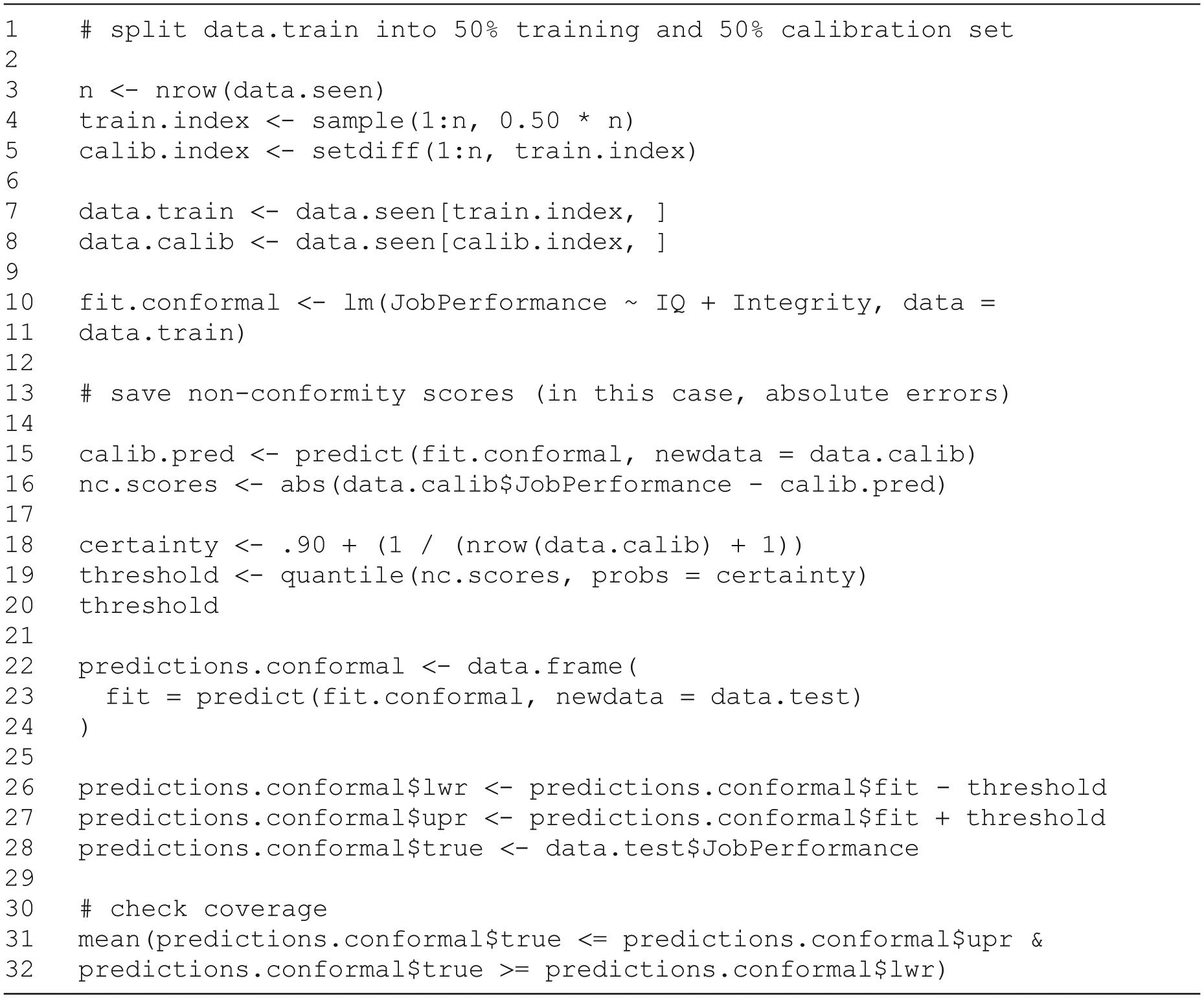
First, the data set containing all available cases for which we have complete data (data.seen) is split into a training set and a calibration set (Table 3, Lines 1–8). We have 1,500 cases available and use 750 randomly selected cases as a training data set that serves as input for the statistical algorithm. We then fit a linear model using the training set (Table 3, Lines 10 and 11).

Now, a certainty level, for example, 90%, must be chosen based on considerations mentioned previously. Here, we assume that the psychologist using the model deemed that the 90% interval would be optimal for choosing job candidates. Next, the model that was fitted to the training data is used to predict the values of the calibration data set using the “predict” function and the “interval = ‘prediction’” option (Table 3, Line 16). From the agreement of predicted and actual values, a nonconformity score is calculated (Table 3, Line 17). These scores are supposed to indicate how “unusual” a particular prediction is compared with the actual value. Nonconformity scores thus should be smaller for more accurate predictions and larger for less accurate ones. In the case of regression, a simple choice would be the absolute difference between predicted and true values, also known as the “absolute error.”

We now have a distribution of nonconformity scores for the calibration data set. From this distribution, we determine a threshold value. By identifying a threshold for nonconformity scores, we effectively determine what constitutes a typical PI for future data. For example, when aiming for 90% coverage, the 90th percentile of the distribution of nonconformity scores is taken (Table 4, Lines 18 and 19). This value, called the “threshold,” is then used to calibrate predictions made for unseen data. A correction factor ( $\frac{1}{N_{c a l i b r a t i o n} + 1}$ ) for finite samples is added to the chosen probability so that we do not underestimate the coverage probability when using small data sets (Angelopoulos & Bates, 2023, p. 3). This will widen the PIs somewhat when the calibration set is small.

Table 4.

Full R Code for Example 2 (Elastic Net Regression)

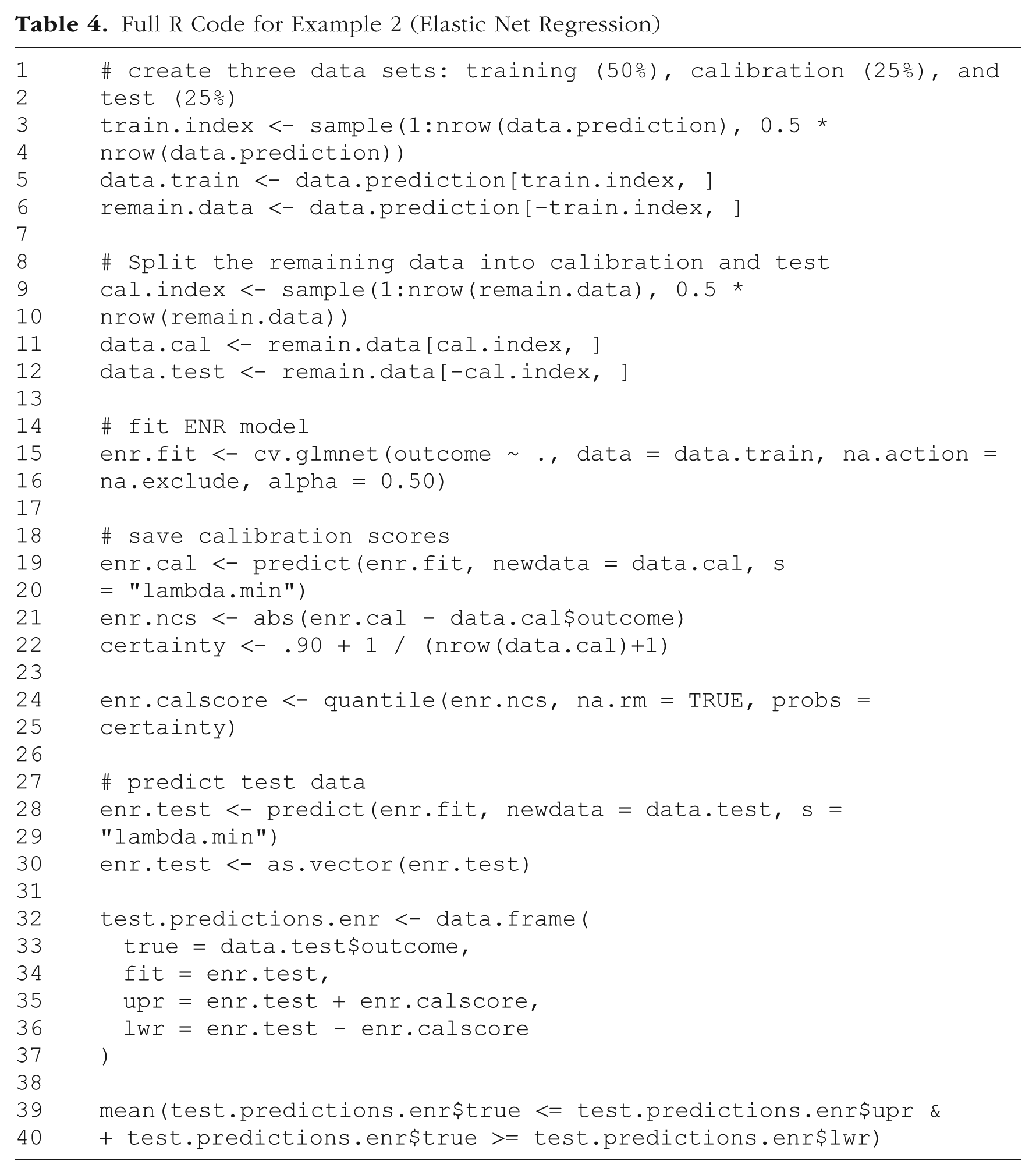
We obtain a threshold of 10.46, which means that predictions with a nonconformity score below this value are considered typical for 90% of cases. Thus, we can use it to compute the bounds of the 90% PI for new, unseen data. The lower bound of the PI for a predicted value is obtained by subtracting the threshold from the predicted value (Table 4, Lines 27 and 28), and the upper bound is obtained by adding it. We now save our predictions for the test set and the corresponding conformal PIs.

By choosing our threshold so that only the 10% “most unusual” predictions lie outside the generated interval, we can assume that this will also be the case for future predictions. Although in practice the test data set is unseen, we are working with a simulated data set and can check the marginal coverage of the generated intervals (Table 3, Line 32). The conformal PIs contained the true value in about 92% of cases.

Figure 1 shows 10 example cases of true job-performance values from the test set and their corresponding 90% PIs. From the 10 intervals displayed, one does not contain the true value.

Fig. 1.

Ten example cases of true job-performance values and prediction intervals. Horizontal lines are 90% conformal prediction intervals. Points are true job-performance values.

Example 2: Elastic Net Regression

In this example, we try to predict the clinical outcomes of a set of digital single-session interventions for adolescents between 13 and 16 years of age evaluated in the COPE trial (Schleider et al., 2022). The data set is available at https://osf.io/8mk6x/. Again, the full R code to reproduce this example is provided in the supplementary material (https://osf.io/d9w8n/; file: EX2_COPE_elastic_net.R). Table 4 shows the R code used in the steps described below.

As the outcome, we chose the primary outcome scale of the study, that is, the Children’s Depression Inventory, second edition, short form (CDI-2; Kovacs, 2011) at the 3-month follow-up. As predictors, we included a set of brief psychometric-scale values measured before the intervention, sociodemographic information (age, sex assigned at birth, gender, race), and the intervention group (three groups: “growth mindset” intervention, behavioral activation, or supportive therapy psychological placebo). Mean imputation was used for missing values in the outcome variable. Missing predictor values were not imputed. For a summary of the descriptive statistics of the included variables, see Table 5.

Table 5.

Descriptive Statistics of All Variables Used in the Examples

	M or n (%)	SD	Minimum	Maximum	Valid n
CDI-2, postintervention	0.97	0.42	0.00	2.00	1,503
CDI-2, baseline	1.19	0.34	0.00	2.00	2,452
Behavioral Activation for Depression Scale	3.04	0.67	0.00	5.44	2,451
Adverse Childhood Experiences Scale	0.48	0.29	0.00	1.00	2,451
UCLA Loneliness Scale	1.96	0.23	0.00	2.75	2,449
State Hope Scale-Agency Scale	3.92	1.41	1.00	8.00	2,452
Generalized Anxiety Disorder Scale	2.99	0.75	1.00	4.00	2,447
Disordered Eating Scale	0.67	0.42	0.00	1.00	2,447
Beck Hopelessness Scale	1.71	0.76	0.00	3.00	2,451
Change in Implicit Personality Theory Questionnaire	3.56	1.28	1.00	6.00	2,451
Multidimensional Peer Victimization Scale	0.70	0.52	0.00	2.00	2,450
Male	251 (10.2%)				2,452
Cisgender	1,567 (63.9%)				2,452
White	1,632 (66.5%)				2,452
Black	257 (10.5%)				2,452
Asian	1,871 (76.3%)				2,452
Hispanic	1985 (81.0%)				2,452
Age (years)	15.12	0.94	13.00	16.00	2,452
Intervention group	Placebo: 818 (33.4%)Behavioral activation: 813 (33.2%)Growth mindset: 821(33.5%)				2,452

Note: Total N = 2,452. CDI-2 = Children’s Depression Inventory, second edition, short form.

Thus, the model included 20 predictors in total. Instead of OLS, we used elastic net regression (ENR; Zou & Hastie, 2005), a regularized regression method that combines LASSO and ridge regression to shrink less relevant parameters. The extent of shrinkage is controlled by the regularization parameter lambda (λ): Higher values result in greater shrinkage. The optimal λ value is determined through cross-validation. The training data set is divided into 10 folds, and for each fold, a model is trained on nine folds and tested on the remaining one. This process is repeated for a range of λ values. The λ associated with the model showing the best predictive accuracy during cross-validation is selected. ENR helps to select only relevant predictors and is especially useful when there are many predictors, some of which may be highly correlated. Obtaining standard errors is not straightforward in ENR, and their validity is contested (Goeman et al., 2022, p. 18), so no PIs with properties similar to those of OLS models can be calculated. This is where the advantage of conformal prediction comes into play, which provides PIs with guaranteed marginal coverage for ENR models.

The data set contained 2,452 cases in total. For the training set, we randomly drew 50% of the data (n = 1,226). From the remaining half, 50% (n = 614) were drawn for the calibration set. The remaining 614 cases were held out to test the coverage of the PIs (Table 4, Lines 1–12).

Using the glmnet package (Friedman et al., 2010), we fit an ENR model to the training data (Table 4, Lines 15 and 16). The model predicts the outcome variable (CDI-2) from all other variables in the data set. The results of this model are summarized in Table 6. The parameters of 15 out of 20 predictors were reduced to zero by the ENR procedure.

Table 6.

Elastic-Net-Regression Results Using CDI-2 at 3-Month Follow-Up as the Criterion

Predictor	b
(Intercept)	0.61
CDI-2, baseline	0.26
Behavioral Activation for Depression Scale	0
Adverse Childhood Experiences Scale	0
UCLA Loneliness Scale	0
State Hope Scale-Agency Scale	−0.001
Program Feedback Scale (PFS)	0
Generalized Anxiety Disorder Scale	0
Disordered Eating Scale	0
Beck Hopelessness Scale	0.04
Change in Implicit Personality Theory Questionnaire	0
Multidimensional Peer Victimization Scale	0.004
Sex: male	0
Gender: cis	−0.03
Race: White	0
Race: Black	0
Race: Asian	0
Race: Hispanic	0
Age	0
Group: BA	0
Group: GM	0

Note: b represents unstandardized regression weights. Reference categories are as follows: sex = female; gender = transgender; race = other; group = placebo. CDI-2 = Children’s Depression Inventory, second edition, short form

The model is now used to predict values from the calibration data set, calculate our calibration scores, and obtain the quantile after correcting it for finite sample size (Table 4, Lines 21 to 24). We used the same model to predict the CDI-2 scores in the test data set (Table 4, Lines 32–37). The calibration score was used to generate PIs.

We now check whether the true values lie within the PI (Table 4, Lines 39 and 40). We do this by calculating the proportion using our previously generated prediction set. In total, 90.4% of values from the test set lie within the PI. As demonstrated, the process of generating PIs is simple and yields intervals with marginal coverage guarantees even when standard methods are not available.

In the previous two examples, the conformal PIs all had the same width because a fixed calibration score was added to and subtracted from each point prediction. However, the uncertainty may vary across different regions of the covariate space—some predictions may require wider PIs to achieve the desired nominal coverage, whereas narrower PIs could be sufficient in other areas. PIs that adjust their width based on local differences in uncertainty are an attempt to achieve conditional coverage, which fixed-width PIs are unable to even approximate. In the next example, we introduce an extension of the previous approach that allows adapting the interval width based on the predicted value.

Example 3: adaptive conformal PIs

In many practical scenarios, the uncertainty associated with predictions can vary depending on the input features, leading to differences in coverage rates depending on predictor values. For example, predictions for extreme or outlier cases are likely to be less reliable than those for data points near the center of the observed distribution. To address this, one can use an adaptive approach that accounts for heteroscedasticity by scaling the nonconformity scores based on the estimated residual variability. In this example, we introduce adaptive conformal PIs using a method based on locally estimated scatterplot smoothing (LOESS) to estimate local uncertainty, allowing the interval widths to adjust dynamically to reflect prediction confidence more accurately. Reproducible R code is available in the supplement (https://osf.io/d9w8n/; file: EX3_COPE_eqr.R), and Table 7 contains the R code for the following procedures.

Table 7.

Full R Code for Example 3 (Adaptive Prediction Intervals Using Locally Estimated Scatterplot Smoothing)

This procedure will add some further steps to our usual procedure, which we demonstrate in this example. However, these are compatible with the prediction methods discussed so far, so we can build on Example 2 and assume that we have performed all the steps up to saving the calibration scores (Table 7, Lines 1–7). Next, however, we use LOESS to model the absolute residuals as a function of the predicted values. Because the predicted value is a combination of the values of the covariates, the residuals of the model are predicted from the fitted values. We then save the LOESS model’s predictions (Table 7, Lines 9–12). We now calculate the nonconformity scores as usual. However, now they will be divided by the square root of the predicted residuals (Table 7, Lines 11–17) and obtain the 90th percentile as usual (Table 7, Lines 19–22).

After we save the predicted values for the test set, we use the LOESS model to estimate the absolute residuals from them (Table 7, Lines 25–30). Finally, we multiply the calibration scores by the LOESS predictions to increase or decrease the PI bounds depending on the expected reliability of the predictions (Table 7, Lines 32–38). We can now check the marginal coverage and see that the desired marginal coverage of 90% was achieved.¹ Also, the widths of the PIs are not fixed but range from 0.89 to 1.65. Figure 2 illustrates this on 10 example cases from the test data set. As is shown, some cases (Cases 533 or 156) have relatively narrow PIs, whereas that of Case 170 is considerably wider.

Fig. 2.

Ten examples for true CDI-2 values and adaptive 90% conformal prediction intervals. Horizontal lines are 90% conformal prediction intervals. Points are true CDI-2 values. CDI-2 = Children’s Depression Inventory, second edition, short form.

Extensions

Conformal prediction is a rapidly developing field. In this tutorial, we focused on providing the basics necessary for application. Various new developments that either extend conformal prediction to new applications (i.e., time-series forecasting) or provide new ways to obtain nonconformity scores are developed regularly. For example, we exclusively used split conformal prediction in this tutorial. This procedure requires splitting the available data into training and calibration data sets. However, an alternative approach is full conformal prediction. Instead of splitting the data and fitting only one model that is later used to make predictions, full conformal prediction uses a leave-one-out procedure. One data point is removed from the full data set, and the remaining data are used to fit the model. This model then predicts the value of the one removed data point, and the nonconformity score is calculated. This process is repeated for every data point. This procedure is computationally highly intensive but can be more efficient and is recommended especially for small data sets because the complete data are available for parameter estimation and calibration. For large data sets, split conformal prediction is still used much more frequently. A compromise solution is cross-validation: Instead of generating a new model for each data point, the data could be divided into 10 equally sized subsamples, for which the calibration process is then repeated accordingly.

During model development, it is advisable that researchers use methods that generate adaptive conformal PIs so that some degree of conditional coverage is achieved. The LOESS-based method we presented in Example 3 is only one possibility to achieve this. Another well-established conformal prediction method is conformalized quantile regression (Romano et al., 2019). For models that directly estimate percentiles of an outcome, conformal prediction can be used to calibrate these percentiles so that they also guarantee marginal coverage. If there are previously known subgroups in the data, it can be helpful to create nonconformity scores within these subgroups rather than from the whole sample.

We also note that conformal prediction is not limited to predicting continuous outcomes. The procedure can also be applied to classification methods, such as logistic regression, for which PIs are normally undefined. Doing this makes it possible to express uncertainty in classification by labeling cases that can be classified as neither positive nor negative. Likewise, classification models for categories with more than two classes can be conformalized so that the user can obtain prediction sets. For example, if a model predicts the probability of five different diagnostic categories, a prediction set might include two of these diagnoses with a probability of 90% and thus exclude the others. For readers interested in applying conformal prediction to classification tasks, we refer to Angelopoulos and Bates (2023, p. 9). For many types of statistical models, conformal-prediction methods are also implemented in the popular R and Python package marginaleffects (Arel-Bundock et al., 2024).

Adaptive conformal inference (ACI) extends conformal prediction to cases in which exchangeability does not hold, such as time-series data or data sets obtained by combining smaller samples. Here, the ordering of data points matters, and exchangeability cannot be assumed. ACI algorithms adaptively generate PIs that factor in the ordering of the data and grow or shrink the resulting PIs. In the R package AdaptiveConformal (Susmann et al., 2023), many ACI algorithms are implemented. With the included functions, the procedures demonstrated in this tutorial can be extended relatively easily to accommodate time-series data.

Discussion

In this tutorial, we introduced the concept of PIs and their relevance for applied research. We then demonstrated a method of generating these intervals using conformal prediction, a distribution-free and model-agnostic method based on relatively liberal assumptions about the underlying data. We have shown that conformal PIs can be generated with only a few easy steps, even for models that lack predefined methods for uncertainty quantification. This is the case for many modifications of linear regression but also for most “black box” machine-learning methods that have become increasingly widespread in psychological research.

The approach is attractive for psychological research for several reasons. The underlying data-generating processes are often unknown in psychology, which leads to inaccurate PIs for many conventional methods. Conformal PIs are adaptable and can be used with any predictive model that can generate point predictions, allowing researchers to judge individual predictive accuracy without worrying about whether their model aligns with a set of assumptions about the data they use. In addition to measures that quantify the accuracy of point predictions (mean absolute error, root mean square error, R²), conformal PIs can also provide a way to compare the accuracy and efficiency of models. A model with narrower conformal PIs is to be preferred compared with a model with wider ones because both models provide the same guaranteed marginal coverage. This is especially useful when choosing among regularized or ensemble models that do not offer native standard errors.

More and more complex statistical models or machine-learning algorithms are increasingly used in psychological research, so robust methods of uncertainty quantification are needed. In many areas of psychology, such models are increasingly being proposed for use in predicting outcomes of new individual cases. For example, research on personalized treatment selection (Cohen & DeRubeis, 2018; Schwartz et al., 2020) has resulted in models that predict outcomes of two or more psychotherapy methods from patient characteristics. We recommend that researchers developing models that are to be used for decisions on individuals report coverage rates and the overall width of PIs. The goal of these models is to serve as a decision-making aid in patient care. Thus, in practice, psychologists must be able to rely on the fact that predictions made by statistical models do not give the false impression of freedom from uncertainty but also that the uncertainty information is reliable. Well-calibrated PIs adequately reflect the uncertainty of predictions and cover the expected proportion of values. Using only point predictions, it is not clear whether the predicted difference in treatment outcome between the two methods is large enough to justify a decision. In many cases, conformal PIs may overlap and, thus, suggest that no clear decision is possible.

As argued by Yarkoni and Westfall (2017), many other applied domains of psychological research strive to make accurate predictions that can in the end be applied to individual cases. Clinical psychologists try to predict outcomes of psychotherapy (Herzog et al., 2022; Kaiser et al., 2023), and industrial-and-organizational psychologists try to enhance the selection of job candidates by predicting job success (Iliescu et al., 2023). But even if prediction does not seem like an obvious task, the use of prediction in new data can provide crucial information about the actual practical implications of the results of psychological research. For example, it is questionable whether a predictor of psychotherapy success that accounts for 8% of the variance in outcome provides relevant insights into the individual probability of a positive outcome. PIs often show quite clearly how much information a predictor or a prediction model provides beyond mere statistically significant parameters. With conformal PIs, this quantification is also possible for more complex models. PIs are already used in the context of meta-analysis (IntHout et al., 2016) to determine the certainty of the evidence for an intervention. In metascience, they can be used to judge inconsistencies of replication studies with previously reported effect sizes (Spence & Stanley, 2024). To our knowledge, conformal PIs have not yet been used in such cases, though.

In general, PIs based on psychological data can be expected to be rather wide because they are often generated from models of noisy data that explain little variance. If the data set is small, the finite-sample correction will increase as well. In such cases, wide PIs are needed to ensure that there is the expected coverage. Diverging from the conventional 95% certainty level established in psychology for significance testing and, consequently, for CIs, can be helpful here. Often, even 85% intervals can already be useful for improving decision-making (e.g., Goodwin et al., 2010). We recommend setting the interval width based on the content considerations of the respective research area. As shown in the first example, the costs and benefits of decisions based on PIs should be considered. In principle, wider intervals will mean that for many cases, no clear decision is possible, whereas for a few cases, the risk of making a wrong prediction is very low. This is recommended for applications in which incorrect predictions are associated with high costs, such as predicting the risk of suicide or the recidivism of violent criminals. There may also be use cases in which it is desirable to have as few cases with unclear decisions as possible. In personnel selection, it may be more economical to make clear decisions even if they include more incorrect predictions.

Furthermore, it is advisable to use adaptive intervals as shown in Example 3 because they can be more efficient for some cases. In general, PIs do not prescribe decisions on their own. Choosing or interpreting PIs requires aligning the statistical output with the substantive context and risk thresholds of the decision problem. The selection and interpretation of PIs ultimately results in the question of how much uncertainty is tolerable in the given context. Although in our tutorial, we focused on the statistical construction of conformal PIs, the substantive use of PIs should be guided by domain-specific considerations, thresholds, or utility functions. In fields such as education or health or job-candidate selection, different trade-offs between coverage and interval width may be acceptable depending on the consequences of error. Decision-theoretic frameworks offer useful tools for formalizing these choices, although practical applications often rely on domain knowledge rather than formal loss functions.

We note some limitations of conformal prediction beyond those already discussed previously. First, conformal prediction requires splitting the available data into training and validation data sets, which reduces the sample size for estimating the model parameters. In small data sets, conventional normal-theory OLS prediction-interval formulas may be preferable to split conformal prediction because they use the full sample for parameter estimation. However, using these comes at the cost of additional assumptions about the data and correctly specified models, which makes the guarantee of marginal coverage less defensible. Second, although conformal prediction provides valid coverage regardless of the accuracy of the underlying model, it does not guarantee that the intervals will be practically useful. If the predictive model has poor accuracy or is strongly misspecified, the resulting PIs may be too wide to support meaningful decisions. Although conformal prediction is a useful tool for quantifying uncertainty, it does not replace the need for well-calibrated, well-specified models. Adaptive methods, as described in Example 3, should be used to ensure that even if intervals are wide on average, they might be practically useful at least for some areas of the feature space. Third, the assumption of exchangeability can be challenged in many practical applications. The obvious case, time-series data, is covered by adaptive methods. More subtle cases are, for example, distribution shifts in unseen data. For example, the demographics of applicants in a company may change significantly. Reweighting methods that are applied during calibration can be helpful for cases of distribution shift in covariates (Tibshirani et al., 2019), but work on efficiently handling many other scenarios that lead to exchangeability violations is ongoing. Finally, it should always be borne in mind that conditional coverage of conformal PIs can only be approximated and cannot be mathematically guaranteed. As already mentioned, this is not a unique disadvantage of conformal prediction but a general property of distribution-free approaches.

Whenever researchers attempt to predict future outcomes and events, they should quantify the uncertainty of their predictions. Conformal prediction represents a significant advance for this purpose. As demonstrated, these methods are compatible with well-established statistical and machine-learning models, further enhancing their utility and accessibility for psychological researchers aiming to improve the interpretability and reliability of their predictive models. Because of the ease with which these methods can be expanded and the lively branch of research they have sparked in recent years, we are confident that they will add an important component to the canon of methods in psychology.

Footnotes

Transparency

Action Editor: Jessica Kay Flake

Editor: David A. Sbarra

Author Contributions

Tim Kaiser: Conceptualization; Data curation; Formal analysis; Investigation; Methodology; Resources; Software; Supervision; Validation; Visualization; Writing – original draft; Writing – review & editing.

Philipp Herzog: Conceptualization; Investigation; Validation; Writing – original draft; Writing – review & editing.

ORCID iDs

Tim Kaiser

Philipp Herzog

Notes

References

Ægisdóttir

White

M. J.

Spengler

P. M.

Maugherman

A. S.

Anderson

L. A.

Cook

R. S.

Nichols

C. N.

Lampropoulos

G. K.

Walker

B. S.

Cohen

Rush

J. D.

(2006). The meta-analysis of clinical judgment project: Fifty-six years of accumulated research on clinical versus statistical prediction. The Counseling Psychologist, 34(3), 341–382. https://doi.org/10.1177/0011000005285875

Angelopoulos

A. N.

Bates

(2022). A gentle introduction to conformal prediction and distribution-free uncertainty quantification. arXiv. https://doi.org/10.48550/arXiv.2107.07511

Angelopoulos

A. N.

Bates

(2023). Conformal prediction: A gentle introduction. Foundations and Trends^® in Machine Learning, 16(4), 494–591. https://doi.org/10.1561/2200000101

Arel-Bundock

Greifer

Heiss

(2024). How to interpret statistical models using marginaleffects in R and Python. Journal of Statistical Software, 111(9), 1–32. https://doi.org/10.18637/jss.v111.i09

Breiman

(2001). Random forests. Machine Learning, 45(1), 5–32. https://doi.org/10.1023/A:1010933404324

Cabezas

L. M. C.

Otto

M. P.

Izbicki

Stern

R. B.

(2025). Regression trees for fast and adaptive prediction intervals. Information Sciences, 686, Article 121369. https://doi.org/10.1016/j.ins.2024.121369

Cohen

Z. D.

DeRubeis

R. J.

(2018). Treatment selection in depression. Annual Review of Clinical Psychology, 14(1), 209–236. https://doi.org/10.1146/annurev-clinpsy-050817-084746

Dewolf

(2024). A comparative study of conformal prediction methods for valid uncertainty quantification in machine learning. arXiv. https://doi.org/10.48550/arXiv.2405.02082

Dewolf

Baets

B. D.

Waegeman

(2023). Valid prediction intervals for regression problems. Artificial Intelligence Review, 56(1), 577–613. https://doi.org/10.1007/s10462-022-10178-5

10.

Friedman

Hastie

Tibshirani

(2010). Regularization paths for generalized linear models via coordinate descent. Journal of Statistical Software, 33(1), 1–22. https://doi.org/10.18637/jss.v033.i01

11.

Goeman

Meijer

Chaturvedi

(2022). L1 and L2 penalized regression models. https://cran.r-project.org/web/packages/penalized/vignettes/penalized.pdf

12.

Goodwin

Önkal

Thomson

(2010). Do forecasts expressed as prediction intervals improve production planning decisions? European Journal of Operational Research, 205(1), 195–201. https://doi.org/10.1016/j.ejor.2009.12.020

13.

Herzog

Feldmann

Kube

Langs

Gärtner

Rauh

Doerr

Hillert

Voderholzer

Rief

Endres

Brakemeier

E.-L.

(2022). Inpatient psychotherapy for depression in a large routine clinical care sample: A Bayesian approach to examining clinical outcomes and predictors of change. Journal of Affective Disorders, 305, 133–143. https://doi.org/10.1016/j.jad.2022.02.057

14.

Iliescu

Ion

Ilie

Ispas

Butucescu

(2023). The incremental validity of personality over time in predicting job performance, voluntary turnover, and career success in high-stakes contexts - A longitudinal study. Personality and Individual Differences, 213, Article 112288. https://doi.org/10.1016/j.paid.2023.112288

15.

IntHout

Ioannidis

J. P. A.

Rovers

M. M.

Goeman

J. J.

(2016). Plea for routinely presenting prediction intervals in meta-analysis. BMJ Open, 6(7), Article e010247. https://doi.org/10.1136/bmjopen-2015-010247

16.

Kaiser

Brakemeier

E.-L.

Herzog

(2023). What if we wait? Using synthetic waiting lists to estimate treatment effects in routine outcome data. Psychotherapy Research, 33(8), 1043–1057. https://doi.org/10.1080/10503307.2023.2182241

17.

Koenker

Hallock

K. F.

(2001). Quantile regression. Journal of Economic Perspectives, 15(4), 143–156. https://doi.org/10.1257/jep.15.4.143

18.

Kovacs

(2011). Children’s Depression Inventory 2nd edition (CDI 2): Technical manual. Multi-Health Systems.

19.

Lakshminarayanan

Pritzel

Blundell

(2017). Simple and scalable predictive uncertainty estimation using deep ensembles. In Proceedings of the 31st International Conference on Neural Information Processing Systems (pp. 6405–6416). Association for Computing Machinery.

20.

Lei

Wasserman

(2014). Distribution-free prediction bands for non-parametric regression. Journal of the Royal Statistical Society Series B: Statistical Methodology, 76(1), 71–96. https://doi.org/10.1111/rssb.12021

21.

Liu

L. T.

Barocas

Kleinberg

Levy

(2023). On the actionability of outcome prediction. arXiv. https://doi.org/10.48550/arXiv.2309.04470

22.

Meehl

P. E.

(1954). Clinical versus statistical prediction—A theoretical analysis and a review of the evidence. University of Minnesota Press.

23.

Papadopoulos

Proedrou

Vovk

Gammerman

(2002). Inductive confidence machines for regression. In Elomaa

Mannila

Toivonen

(Eds.), Machine learning: ECML 2002 (pp. 345–356). Springer. https://doi.org/10.1007/3-540-36755-1_29

24.

Romano

Patterson

Candes

(2019). Conformalized quantile regression. Advances in Neural Information Processing Systems, 32. https://proceedings.neurips.cc/paper/2019/hash/5103c3584b063c431bd1268e9b5e76fb-Abstract.html

25.

Schleider

J. L.

Mullarkey

M. C.

Fox

K. R.

Dobias

M. L.

Shroff

Hart

E. A.

Roulston

C. A.

(2022). A randomized trial of online single session interventions for adolescent depression during COVID-19. Nature Human Behaviour, 6(2), 258–268. https://doi.org/10.1038/s41562-021-01235-0

26.

Schwartz

Cohen

Z. D.

Rubel

J. A.

Zimmermann

Wittmann

W. W.

Lutz

(2020). Personalized treatment selection in routine care: Integrating machine learning and statistical algorithms to recommend cognitive behavioral or psychodynamic therapy. Psychotherapy Research, 31(1), 33–51. https://doi.org/10.1080/10503307.2020.1769219

27.

Schweder

Hjort

N. L.

(2016). Confidence, likelihood, probability: Statistical inference with confidence distributions. Cambridge University Press. https://doi.org/10.1017/CBO9781139046671

28.

Spence

J. R.

Stanley

D. J.

(2024). Tempered expectations: A tutorial for calculating and interpreting prediction intervals in the context of replications. Advances in Methods and Practices in Psychological Science, 7(1) https://doi.org/10.1177/25152459231217932

29.

Susmann

Chambaz

Josse

(2023). AdaptiveConformal: An R package for adaptive conformal inference. arXiv. https://doi.org/10.48550/arXiv.2312.00448

30.

Tibshirani

R. J.

Foygel Barber

Candes

Ramdas

(2019). Conformal prediction under covariate shift. Advances in Neural Information Processing Systems, 32. https://papers.neurips.cc/paper_files/paper/2019/hash/8fb21ee7a2207526da55a679f0332de2-Abstract.html

31.

Vos

Holbert

(2022). Frequentist statistical inference without repeated sampling. Synthese, 200(89), 1–25. https://doi.org/10.1007/s11229-022-03560-x

32.

Vovk

Gammerman

Shafer

(2005). Algorithmic learning in a random world. Springer. https://doi.org/10.1007/b106715

33.

Xie

(2021). Conformal prediction interval for dynamic time-series. Proceedings of Machine Learning Research, 139, 11559–11569. https://proceedings.mlr.press/v139/xu21h.html

34.

Yarkoni

Westfall

(2017). Choosing prediction over explanation in psychology: Lessons from machine learning. Perspectives on Psychological Science, 12(6), 1100–1122. https://doi.org/10.1177/1745691617693393

35.

Zou

Hastie

(2005). Regularization and variable selection via the elastic net. Journal of the Royal Statistical Society Series B: Statistical Methodology, 67(2), 301–320. https://doi.org/10.1111/j.1467-9868.2005.00503.x

A Tutorial on Distribution-Free Uncertainty Quantification Using Conformal Prediction

Abstract

Keywords

Uncertainty in Predictions

Quantifying uncertainty using prediction intervals

From point predictions to PIs

From PIs to decisions

Challenges With Traditional Methods

Alternative Methods for PIs

Conformal Prediction

General approach

Marginal and conditional coverage

Assumptions

Sample size

Comparison with standard methods

Example 1: general procedure

Example 2: Elastic Net Regression

Example 3: adaptive conformal PIs

Extensions

Discussion

Footnotes

Transparency

ORCID iDs

Notes

References