
Abstract
Large language models (LLMs) are transforming research in psychology and the behavioral sciences by enabling advanced text analysis at scale. Their applications range from the analysis of social media posts to infer psychological traits to the automated scoring of open-ended survey responses. However, despite their potential, many behavioral scientists struggle to integrate LLMs into their research because of the complexity of text modeling. In this tutorial, we aim to provide an accessible introduction to LLM-based text analysis, focusing on the Transformer architecture. We guide researchers through the process of preparing text data, using pretrained Transformer models to generate text embeddings, fine-tuning models for specific tasks such as text classification, and applying interpretability methods, such as Shapley additive explanations and local interpretable model-agnostic explanations, to explain model predictions. By making these powerful techniques more approachable, we hope to empower behavioral scientists to leverage LLMs in their research, unlocking new opportunities for analyzing and interpreting textual data.
Keywords
Over the past decade, the application of machine learning (ML) in the behavioral sciences has opened up new possibilities for modeling and understanding human behavior and latent psychological constructs. Tasks that once relied on manual data processing are now being automated, allowing researchers to analyze vast amounts of information with greater precision and scale. One of the most impactful areas of application where this shift is occurring is natural language processing (NLP), which enables computers to interpret, analyze, and generate human-language data (Goodfellow et al., 2016). NLP has become a powerful tool that helps behavioral scientists perform a wide range of tasks, from the analysis of social media posts for the detection of sentiment changes to the scoring of open-ended survey questions to inferences of psychological traits (Tunstall et al., 2022).
However, alongside the rapid evolution of NLP methods, behavioral scientists face the challenge of how to integrate these complex tools into their research workflow. The advent of large language models (LLMs), such as Transformer models, have revolutionized NLP and offer unprecedented possibilities for the understanding of human thoughts, feelings, behavior, and context through language. Despite their potential, many researchers find it difficult to apply these models because of technical barriers and a lack of accessible, practical guidance. In this tutorial, we aim to bridge this gap by offering an accessible, step-by-step introduction to LLMs. In the remainder of this article, we first provide an optional introduction to the Transformer-model architecture, an overview of LLMs, and their application to analyze text data in the behavioral sciences. In the second part of the article, we present a practical, interactive tutorial with coding exercises demonstrating how to perform LLM-based text analysis.
The Transformer Architecture
Neural networks (NNs) are a powerful class of ML models capable of processing complex inputs, such as images or text, through multiple layers of nonlinear transformations, enabling them to solve a wide range of tasks (Goodfellow et al., 2016). Originally inspired by biological structures in the human brain (i.e., neurons), NNs have considerably evolved over the past years; newer (more extensive) architectures are referred to as “deep learning” (DL) models. Transformer networks (Vaswani et al., 2017) are a special type of NN that allows parallel processing of sequential data formats such as text; in this framework, text can be considered sequential because it is generally processed (“read”) in a specific direction. “Parallel processing” in this context means that these models can simultaneously handle multiple parts of the input (here: parts of the text) instead of serially. Transformers were initially developed as a combined encoder–decoder model for (neural) machine translation of texts (Sutskever et al., 2014). Here, an encoder part is followed by a decoder. The encoder part of a Transformer maps the individual parts of the input (i.e., the tokens 1 of a text in the source language) to so-called embeddings. There are condensed numerical representations of the original tokens. In overly simplified terms, one can think of embeddings as numerical vectors (similar to component loadings in a principal component analysis). As vectors, they can also be seen as points that help to determine the position of a token in the larger context of all text that has been used to train the model. For instance, the embedding for “king” should be closer to that of “queen” than to that of “apple.” In that sense, embeddings provide useful numeric representations of the meaning of the token contained in a given text. Some readers may be familiar with earlier methods, such as Word2vec (Mikolov et al., 2013), which produce static embeddings for words or tokens. In contrast, Transformer-based embeddings are contextual, which means that they are able to consider the specific context a word is used in. As a consequence, the same word can have different embeddings depending on the surrounding text. One important application of these embeddings, which is outside the scope of this article, involves semantic comparisons of words or word parts (cf. Kjell et al., 2023). These embeddings can, for example, capture individuals’ affective or cognitive state based on their language use. In the subsequent decoding phase, these internal representations can be accessed and used to generate a target sequence (e.g., a translation). As we show, these representations can also be used to predict or generate relevant psychological insights, such as identifying underlying emotions or behavioral tendencies from text. Figure 1 summarizes the original encoder–decoder nature of the Transformer-model architecture (Vaswani et al., 2017).
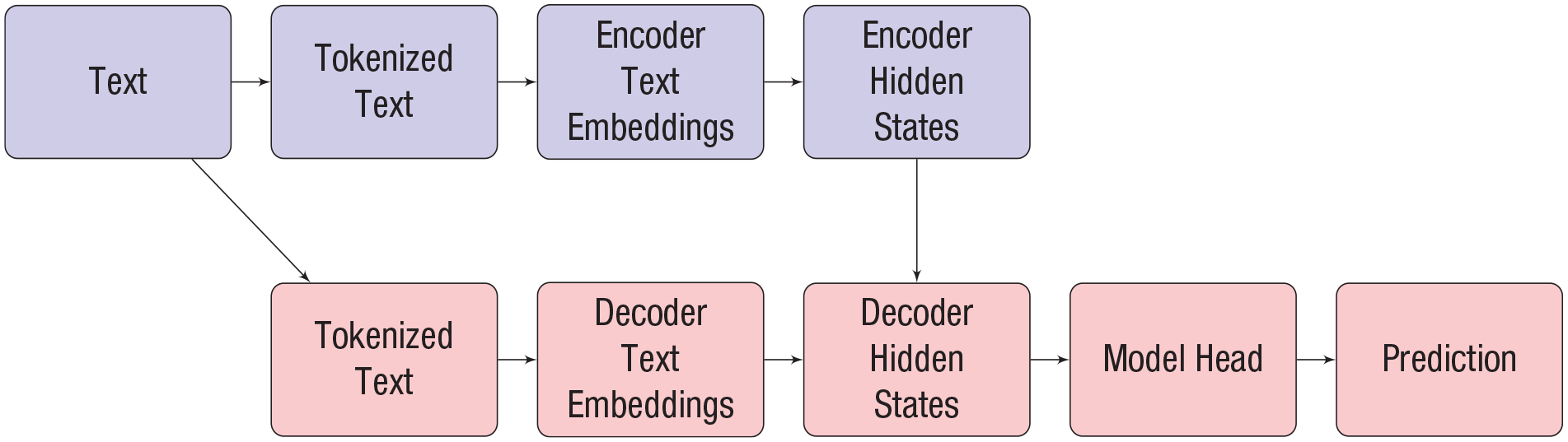
The basic Transformer architecture, adapted from Tunstall et al. (2022). The top row represents the encoder, and the bottom row represents the decoder.
The basic aim of the original Transformer architecture consists of taking a sequence (e.g., text) as input and producing a sequence as output. Both of these sequences can be of arbitrary length, making Transformers ideally suited for tasks such as machine translation (e.g., a sentence in German as input and a sentence in English as output), summarization (e.g., a long sentence as input, a word as output), or question answering (e.g., a question as input, an answer as output). Its major innovation was the isolation of the attention mechanism (Bahdanau et al., 2015). The basic idea of the attention mechanism in the encoder (“self-attention”) is to iteratively refine and enhance the contextual representations of individual tokens. The attention mechanism connects the encoder and decoder (“cross-attention”) and then allows the generation of new text by considering the embeddings provided by the encoder.
LLMs: An Overview
To provide the reader with a broader overview, we present some of the most commonly used (pretrained) LLMs based on the Transformer and elaborate on how they correspond to solving the task at hand. An overview of some common open-source Transformer models is also provided in the Supplemental Material available online. Soon after the invention of the Transformer, researchers started using its encoder and decoder parts separately for distinct purposes.
As illustrated in Figure 2, encoder-based 2 models dominated the landscape from 2018 to 2020, leveraging the self-attention mechanism of the Transformer to learn contextualized representations that can be used to classify individual tokens or text sequences. The launch of GPT-3 (Brown et al., 2020) in mid-2020 ignited a paradigm shift away from simple classification to harness the generative nature of decoder-based models (cf. Fig. 2). This included using decoder-based models for creative writing (Radford et al., 2019) and other tasks related to text creation, but (at the latest) the introduction of GPT-3 showed that these models could also be leveraged for classification efficiently. Finally, the complete encoder-decoder model class also sparked some developments of influential models early on (Raffel et al., 2020; Wei et al., 2021). As opposed to encoder-based models (for which developments have nearly stopped altogether), there are still active developments for the encoder-decoder model class alongside the growing dominance of Transformer decoder-based models. For other recent reviews of the architecture underlying the Transformer models, see Tunstall et al. (2022), Yang et al. (2023), or Hussain et al. (2024). Nowadays, many of these models are summarized under the term “LLMs” or “foundation models” (Bommasani et al., 2022). 3 The term “LLM” has evolved over time and is now commonly used to describe large, pretrained models. In this article, we categorize all large, pretrained, Transformer-based models as LLMs. Decoder-based models, commonly used for generative tasks, are specifically referred to as “generative” LLMs. A list of some commonly used Transformer-based models is presented in the Supplemental Material.

Illustration of large-language-model developments based on the Transformer architecture (Yang et al., 2023).
Encoder models
The initial use case for encoder-based models was to achieve better representation learning capabilities (i.e., better quantification of the meaning of words in their context). This resulted in a class of models ideally suited for (a) sequence-classification tasks (e.g., sentiment analysis) or (b) tagging tasks (i.e., classification of individual tokens). An example of a tagging task is named “entity recognition,” which involves identifying and classifying key information (entities), such as persons or places, in a text (e.g., identifying people in conversations or masking names and other confidential information). Important Transformer models that belong to this type of architecture are BERT (Devlin et al., 2019) and its creative variations, such as RoBERTa (Liu et al., 2019), ALBERT (Lan et al., 2020), or DistilBERT (Sanh et al., 2020). BERT essentially learns how to contextualize the information contained in written text via its pretraining tasks. DistilBERT is designed to be a smaller and faster model than BERT that is still comparatively powerful, and ALBERT is also designed more efficiently. RoBERTa, on the other hand, is a variation of BERT that differs in some key hyperparameters from the original model. Compared with the original BERT model, RoBERTa performs better in most tasks, and we can safely recommend its use instead of BERT. Although these models focus on the evaluation of English texts, there are also variations available that are trained on other languages and other corpora. Most recently, a “modern” version of BERT, called “modernBERT” (Warner et al., 2024), was published in late 2024, making use of all the advancements that have happened since the training of the “original” BERT in 2018.
Decoder models
The second type of model consists only of the decoder part and is most useful for generative tasks, for instance, in the context of text completion or generation. Widely known variants are the models from the GPT series, that is, GPT (Generative Pretrained Transformer; Radford et al., 2018) to GPT-4 (OpenAI, 2023). These models became extremely popular with the introduction of the conversational ChatGPT interface (OpenAI, 2022) and can be used for a wide range of tasks. However, we do not focus on GPT models in this tutorial. Although text classification in a zero- or few-shot setting 4 is also possible with this model class, this application comes with several new hyperparameters and implications that go beyond the scope of this work. Instead, we want to enable applied psychologists to use cheap but powerful NLP models for classical ML in their research. Therefore, we focus on (a) the software tools for (b) fine-tuning encoder-based text-classification models. Thus, we do not discuss decoder-based models in greater detail here, but a thorough understanding of this tutorial will be beneficial for getting started on decoder-based models.
Encoder–decoder models
The third type of Transformer-based model consists of the originally proposed model, that is, encoder and decoder. The encoder–decoder architecture is useful for establishing complex mappings between sentences, which are required for summarizing or translation tasks. However, given the increasing context length that decoder-based models can incorporate, most of these tasks can now be solved by providing them with the input sequence as a prompt, 5 leading to an increased use of decoder-only models. Important representatives of pretrained encoder–decoder models include BART (Lewis et al., 2019) and T5 (Raffel et al., 2020), which can be used for applications involving text generation.
Accessing Transformer models via Hugging Face
A central contemporary way to access open-source Transformer models such as those mentioned in the previous paragraphs is the Hugging Face Hub. Hugging Face is an open-source platform providing state-of-the-art tools for NLP and DL. Following Tunstall et al. (2022), this ecosystem consists of two central parts; the first is the Hugging Face Model Hub, and the second is several Python libraries, in particular,
The mentioned Python packages help with handling models and processing data: The
Recent developments
LLM research has focused on scaling so-called “test-time compute” to enhance performance while saving computational resources in pretraining. Research indicates that by optimally increasing computational resources during inference, models can achieve superior results without the necessity of more exhaustive or larger parameter counts of the underlying model. Here, “inference” refers to the phase in which a trained model processes new data as input to generate predictions or classifications of other output. This approach has been shown to outperform larger models when evaluated under equivalent computational constraints (Snell et al., 2024). As of the writing of this article, the most notable recent developments regarding models are the openly available DeepSeek-R1 (DeepSeek-AI et al., 2025) and OpenAI’s o1 commercial model. DeepSeek-R1 uses novel reinforcement learning techniques that achieve high performance while minimizing computational costs. Another trend is using LLM-generated data for training, such as for DeepSeek-R1, which has been shown to enhance their performance in tasks related to reasoning capabilities. However, this practice also raises concerns about data quality and potential feedback loops, calling for careful validation (Alemohammad et al., 2023). These recent developments and innovations highlight the rapid evolution of contemporary LLMs, underscoring both the potential and the challenges associated with their training and deployment.
LLM-Based Text Analysis
After having introduced the theoretical foundation of the Transformer architecture, we now outline the concrete steps that are necessary to use a Transformer model, such as BERT (Devlin et al., 2019), for the creation of embeddings, the prediction of criteria, and fine-tuning and interpretation.
Step 1
The first step typically consists of importing the data and applying additional preprocessing. Unlike many other NLP methods (Kennedy et al., 2021), the application of Transformer-based models does typically not require specific preprocessing steps such as the removal of frequent words (so-called stop words), stemming (i.e., removing word endings), or lemmatization (i.e., returning words to base form) of words in the corpus. As an exception, it might be necessary to remove special characters (e.g., from links and hashtags) so that the form of the processed text corresponds to what the model requires as input.
Step 2
The second step is the tokenization of the text. Transformer-based models break text into tokens and map these tokens to integer indices representing the input. Typically, tokens represent the indices of word parts in the predefined vocabulary of a tokenizer. For example, consider the sentence “I am happy,” which consists of the words “I,” “am,” and “happy.” It can be tokenized as a series of indices, such as [13,27,98,1], with each index standing for a word or word part; in this example, the indices were chosen arbitrarily but depend on the type of tokenizer. In the example, 13 represents “I,” 27 represents “am,” and 98 represents “happy” in this specific sentence.
Additional tokens can have a special meaning ([CLS] in BERT), can mark the end of sequences ([SEP] in BERT), or may be used to represent unknown words that were not part of the model’s pretraining corpus ([UNK] in BERT). In the example given above, “1” represents the end of the sentence. The special token [CLS] added at the beginning of a sentence has the purpose of summarizing the meaning of a sentence and is used for classification tasks, as its name indicates. The overall process of obtaining tokens from words is called “tokenization” and is carried out by “tokenizers,” which are software functions designed for this purpose. Tokenizers are specific to a given model. Tokenization is a data-driven process in which the vocabulary of the tokenizer is iteratively defined given a corpus of text and some hyperparameters (Sennrich et al., 2016; Y. Wu et al., 2016). Using the correct tokenizer for a pretrained Transformer model ensures that text is processed consistently with its training.
In this tutorial, we use Hugging Face as a platform to apply Transformer models. On a technical level, tokenizers from the
Step 3
In the third step, tokens are transformed into embeddings, which capture their meaning and serve as input for deeper layers of the Transformer-based LLM. Depending on the application, one can use these embeddings for at least two strategies, representing the fourth step of our analysis.
Step 4: Strategy 1
In the first strategy, the Transformer models act as feature extractors 7 ; tokens are processed by the first layers of a pretrained LLM to extract vector representations of the text. During the pretraining on extensive text corpora, they can learn powerful representations in a self-supervised 8 manner. For instance, the encoder-based model BERT (Devlin et al., 2019) has been pretrained using two self-supervised tasks—the masked-language modeling 9 and next-sentence prediction 10 —on data from the BooksCorpus (Zhu et al., 2015) and from Wikipedia. Pretraining allows BERT to convert text into meaningful numerical representations (embeddings) that capture semantic relationships. It can do this even for new texts as long as they are similar to the data it was originally trained on. 11 In this feature-extraction strategy, the LLM itself is not adapted (i.e., changed by the data processing), and the extracted features are used in a separate classification model as predictors. This strategy is computationally cheap and applies Transformer models merely to provide numerical vectors that aim to capture the meaning of the text. In the model in Figure 1, the feature-extraction strategy corresponds to using the hidden states provided by a pretrained encoder or decoder as input for a separate ML model, such as a regularized regression model or a random forest, which is trained for the task at hand. Recent work has used this technique (e.g., Koch et al., 2024).
Step 4: Strategy 2
As a second strategy, the classification model is directly integrated into the pretrained LLM by adding a task-specific layer on top of the Transformer and further training it. 12 This adaption to specific classification problems is called “fine-tuning,” turning the powerful feature extractors (cf. Strategy 1) into a usable classifier for the custom problem at hand (e.g., emotion classification from text). This approach allows the model to leverage custom, labeled training data to apply the knowledge gained during pretraining to specific tasks. The much more expensive pretraining has to be executed only once (and is usually done by organizations with access to extensive computational resources), and the (relatively) cheap fine-tuning can be performed by individual researchers using fewer computational resources. A simplified yet helpful analogy to this process can be to think of a production process in which trees are processed into wooden bars that can be used for a broad range of tasks (cf. pretraining). At a later stage, the wooden bars can be further processed into tools or furniture that are better suited for specific purposes (cf. fine-tuning). However, fine-tuning is still usually computationally more expensive than just feature extraction from the pretrained model yet often leads to better results. Fine-tuning can vary in the extent of this adaptation. In extreme cases, it can mean just training a linear classifier on top of the pretrained model’s representations (i.e., embeddings), which corresponds to Strategy 1 outlined in this article, or updating the entirety of the model’s weights. Although the former is the computationally cheaper approach, the latter often results in superior performance, as stated by Tunstall et al. (2022, Chapter 2).
Step 5
In an optional final step, we can use interpretable ML (IML) methods to explain the predictions (i.e., the predicted classes in a classification task; Molnar, 2022). In this tutorial, we gently guide the reader through all these steps. We also provide a summary of important terminology used in NLP and ML in the Supplemental Material.
Current Applications of LLMs in the Behavioral Sciences
Researchers in psychology and the behavioral sciences in general have been increasingly adopting LLMs for scientific investigations. A comprehensive review of existing and potential applications in the field was provided by Demszky et al. (2023) and Feuerriegel et al. (2025). One key application is the quantification of textual data through embeddings in relation to a psychological construct of interest. These embeddings, often aggregated (e.g., by taking the mean), can serve as features in predictive models that aim, for example, to infer psychological traits and states (Koch et al., 2024; Mehta et al., 2020; Sust et al., 2023). Recent approaches leverage pretrained LLMs in zero-shot-learning scenarios, applying them to tasks such as inferring personality traits from social media data and generating content for personalized experimental conditions (Peters & Matz, 2024). In addition, LLMs have been applied to quantify brand perceptions (Hartmann et al., 2023) and to automatically grade human-generated text, thus alleviating some of the routine burdens on educators. Moreover, LLMs have supported clinical decision-making by analyzing language and speech patterns to identify potential health risks (Crema et al., 2022). For instance, LLM-based speech-analysis methods have been applied to assess Alzheimer’s-disease risk and detect early signs of psychosis and schizophrenia (Corcoran & Cecchi, 2020; Gashkarimov et al., 2023; Ilias & Askounis, 2022; Khan et al., 2022; Kong et al., 2021; Roshanzamir et al., 2021). LLMs are also valuable for generating content that enhances or even replaces traditional assessment tools. In personality psychology and psychological diagnostics, these models have been used to generate new questionnaire items and enable open-text assessments, replacing traditional item-based formats with more flexible response options (Götz et al., 2024; Kjell et al., 2022). Likewise, in educational settings, LLMs have been applied to create new assessment items (Hommel et al., 2022; von Davier, 2018). Hence, LLMs’ generative capabilities support a range of educational functions, including generating feedback and recommendations and even assisting teachers with content creation (Yan et al., 2024). In consumer psychology, LLMs have been used to create content optimized for search engines and even generate synthetic participant data (Li et al., 2024; Ma et al., 2024; Reisenbichler et al., 2022). On a larger scale, LLM-generated content allows for personalized persuasive messaging (Matz et al., 2024). These examples show how LLMs can serve as powerful tools capable of addressing a wide range of tasks—from diagnostic support to content generation and automated assessment—across various fields in the behavioral sciences.
So far, we have covered the foundational concepts and functionalities of the Transformer architecture on a rather theoretical level and equipped the reader with an overview of useful applications of LLMs. We also provided an overview of the central steps for LLM-based text analysis. In the following practical sections, we apply LLM-based text classification in four consecutive modules: We (a) provide a conceptual overview of LLMs and the underlying Transformer architecture, (b) demonstrate how a textual data set can be loaded in Python, (c) show how a pretrained Transformer model can be used to create text embeddings that can be used as predictors/features in a predictive model, (d) explain how an existing Transformer model can be fine-tuned for a specific task (e.g., text classification), and (e) illustrate how methods of IML can be used to understand the predictions of a model.
However, given the breadth of this research field, in this tutorial, we do not cover all the details of NLP, ML, and DL. Therefore, we want to point the reader to several related and highly relevant articles. For a theoretical introduction to DL, we recommend Urban and Gates (2021). For an introduction to NLP in the context of DL, we refer to Tunstall et al. (2022) and Eisenstein (2019). Kennedy et al. (2021) provided a general overview of text-analysis methods for psychologists. In relation to more fundamental topics, we strongly recommend the supervised-ML tutorial for psychologists by Pargent et al. (2023) and the IML tutorial by Henninger et al. (2025).
Module 1: Data Preparation for Modeling With Transformers
Technical setup for the tutorial
To facilitate hands-on exploration, we provide an interactive Jupyter Notebook, designed primarily for use with Google Colab. 13 To use it, readers can simply open the link and sign in with a Google account. We also offer an alternative version based on ModernBERT. 14
For readers who prefer running the notebook locally, the full implementation is available in an OSF repository: https://osf.io/9de3m/. To run the notebook in Google Colab with a local copy, first download it from OSF and then upload it by clicking “File” and “Upload Notebook” within Colab.
In addition, we provide an R implementation using the
The Colab notebook and the Python and R files allow readers to carry out the main steps of the analysis in parallel to reading the text—a practice we strongly encourage. Before starting the analysis, ensure that the required Python packages are installed. These include
Data sets used in the practical exercises
In this tutorial, we use a small, illustrative data set of 100 speech transcripts that were collected among students at the University of Texas at Austin (C. Wu et al., 2021). During a 3-week self-tracking assignment, participants received four short experience-sampling questionnaires per day and could also record their voice with their smartphones. In the experience-sampling procedure, self-reported contentment was assessed on a 4-point Likert scale, among other psychological properties. For the audio records, participants received the following instruction: “Please record a short audio clip in which you describe the situation you are in and your current thoughts and feelings. Collect about 10 seconds of environmental sound after the description.” Any parts of the record that did not contain speech were cut out before the analysis. The collected speech samples were also analyzed in other research projects, which describe the data-collection procedures in greater detail (Koch et al., 2024; Marrero et al., 2022). Raw audio records were transcribed using the Google speech-to-text API (Version 1). For this tutorial, we selected transcripts between 45 and 55 words in length and cases of low or high self-reported contentment. Finally, we randomly selected 50 of those high- and low-contentment transcripts each. This categorization of the answers in low versus high makes this a binary-classification problem, one of the most common and illustrative use cases for training ML classifiers.
Loading the data
Because our study focuses on text classification (i.e., prediction of a categorical outcome) using Transformer models, we attribute all text responses to one of two categories (i.e., high vs. low contentment). We also briefly mention how to adapt the code for regression problems, that is, the prediction of continuous outcomes. We now want to predict high or low contentment based on the short texts provided by the respondents. Therefore, the classification task consists of predicting the category of each text based on the text content, that is, the list of reported words. Based on the overall sample of 100 observations, we randomly assigned 80 responses to the part of the data set that we use for training the predictive models (cf. training set). The remaining 20 responses serve as the test set, which is used for the final evaluation of model performance and for comparison with other models. We provide the necessary .csv files containing the train and test sets in our OSF repository: https://osf.io/9de3m/?view_only=214a0d84044644a1a7405308e18b7df1. We start our tutorial by loading the software packages that are relevant for loading the data sets:

The Jupyter notebook and the R files that accompany this text further contain additional code to download the
Next, we load the training and test data sets. We later split the training set further into a smaller training set and a validation set. We then specify two arguments: the symbol separating the columns containing the text and labels, which is “;”, and the names of the two columns, “
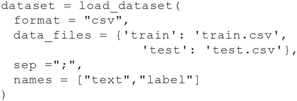
In our example, the data are available as .csv files with semicolons used for separating the texts and labels. Because multiple other types of files could also be used to store the data, the
Both data sets contain short texts that were provided by respondents to describe their current level of contentment and the binary target variable of the classification task (contentment). For instance, the text of the first response of the training set is given by the following text: I’m kind of down right now because I was late to my chem class this morning. So I’m feeling really sad about that cuz I miss my homework selection, my turn in and now I’m just try to get over it and I’m just sitting at home.
This response is assigned the label “0,” which stands for low contentment. A high level of contentment corresponds to a label of “1.”
With the following code chunk, we load the tokenizer for a specific Transformer model, that is, the English DistilBERT model (Sanh et al., 2020). This model is labeled as “uncased” because it does not consider the case of texts, that is, whether letters are uppercase or lowercase. We discuss this Transformer model in more detail in the next section. For now, it is sufficient to know that this model can be used for the task at hand while being computationally efficient:

Following the approach described by Tunstall et al. (2022), we define a tokenizer function

We now use this function to tokenize the complete data set, which includes the training set and test set. As a result of the tokenization, the raw text is transformed into integer values, so-called tokens, which can be further processed. We now explain the remaining arguments of the following

After this step, the first instance of the training set contains two additional entries, which are (a) a series of 62 tokens, which are integer values, and (b) the attention mask, which indicates the positions of padding tokens in the data to exclude them from contextualization. Note that the number of tokens is larger than the number of words (51) because the tokens generated by this tokenizer are based on parts of words. The next step in our analysis is the application of a Transformer model to predict contentment scores from the provided text.
Module 1 summary
This initial step focused on data preparation. We loaded the raw data and converted it into a format suitable for the DistilBERT model by applying its tokenizer function. In the following second module, we use the processed tokens for text classification using the two distinct strategies outlined in the introduction.
Module 2: Applying a Pretrained Transformer Model for Text Classification
Transformers as feature extractors
We use the English DistilBERT to obtain word embeddings for the response texts in our data set, chosen for its suitability for text-sequence classification, focus on English, and relatively small size. In practical applications, it might be useful to compare the performance of this model, as measured by its accuracy on the test set, against that of other Transformer-based models.
To apply Transformer models such as DistilBERT in the context of the Hugging Face ecosystem, it is necessary to use a software framework for training DL models. Many of those have been developed in private companies. In this case, we apply PyTorch (Paszke et al., 2019), which was developed by researchers at Meta. This selection is somewhat arbitrary, and a common alternative is TensorFlow (Abadi et al., 2015), which was developed by Google Brain. In the following lines of code, we import PyTorch (Python package:

As a next step, we define the function

In the next line of code, we convert our tokenized data set,

Finally, we obtain the hidden states (i.e., the embeddings) by applying

Using embeddings as features
The word embeddings that resulted from the previous step will now serve as features for a subsequent ML model. In our application, we use a logistic ridge regression model (James et al., 2023) as a secondary ML model. Conceptually, this model is comparable with a logistic regression but aims at providing a model in which the sum of the squared regression coefficients is small while still providing a high goodness of fit to the data (via regularization). A similar approach was used by Kjell et al. (2023). This model choice was motivated by the heuristic assumption that some entries of the most word embeddings might not be useful for predicting the contentment score. A second argument for using a regularized regression model is that such a model might prevent overfitting, that is, the model shows a high accuracy on the training data but a much lower accuracy on the test set. Conceptually, overfitting means that the model has learned rules and patterns that are specific to the training data but do not generalize well to new data (i.e., noise). It is therefore essential to prevent overfitting to obtain realistic estimates of model performance. In the data set at hand, this point is particularly important because we have 768 features but only 80 observations.
Naturally, we could also choose a more complex ML model to learn the statistical relationship between the word embeddings and the target variable, such as random forests. Random forests can model more complex relationships than a logistic ridge regression model, but they are more difficult to interpret (James et al., 2023). To follow the strategy outlined above, we first transform the word embeddings and the labels of the texts into

We now have the hidden states of the training and test sets as


The “CV,” as in RidgeClassifierCV, stands for cross-validation, an essential resampling technique for model evaluation, which aims to prevent overestimating the model performance. The

We obtain an accuracy of 0.825 in the training set and 0.85 in the test set. We can inspect the optimal value for alpha that was found in the cross-validation via

We can also obtain the regression weights via

However, we note that these regression weights correspond to the elements of the word-embedding vector of the [CLS] token, which summarizes the complete text. Therefore, they cannot be directly interpreted as the influence of individual words.
The accuracy in the test set can be seen as an estimate of the model performance on new data when the first strategy is used. This value is often but not always lower than the accuracy observed on the training set, which was 0.825 in our case. In predictive modeling, it is essential to always compare model performances with reasonable baselines. In the context of this study, 0.85 is above the accuracy that could be expected if we had naively predicted the most common label. Because both labels are almost equally common in our training set, this would have led to an accuracy of about 0.5. On the other hand, 0.85 might not be accurate enough for all practical applications in social and behavioral sciences, for instance, in the context of psychological assessments on the level of individuals. For obtaining higher accuracy, one might even use alternative ML models, tune the hyperparameters of these models, or collect a larger data set. Data acquisition is often the most computationally expensive part of training an ML model. However, collecting more data helps the model learn complex patterns, leading to more accurate predictions. To learn more about all steps in basic ML modeling for psychology, refer to Pargent et al. (2023).
Module 2 summary
In this second module, we used DistilBERT to extract embedding features that we used as predictors in a regularized logistic regression to predict binary contentment.
Module 3: Fine-Tuning Transformers for Classification
Fine-Tuning as Alternative Strategy
In this module, we use a classification model directly based on DistilBERT but fine-tune it to the task. This strategy is computationally more expensive than the strategy based on feature extraction and also leads to a deeper classifier with more layers. However, this approach allows for greater flexibility by adapting the Transformer model to the specific task as more model components, outlined in Figure 1, are adjusted accordingly. We start by splitting our original training set into a new, smaller version (80% of the original training data) and a validation set (20% of the original data) because cross-validation is usually too expensive for evaluating fine-tuned models:

We proceed by defining the number of labels to predict and loading the pretrained DistilBERT model. In this case, we have two labels—0 and 1:
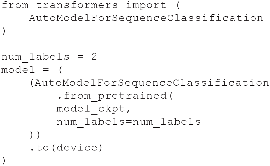
If we were to predict more than two groups, we would need to adjust
In contrast to the pretrained model used in the first strategy, this model not only provides a final layer that can be used for extracting word embeddings but also includes an additional final layer that allows for the direct prediction of the two labels. In Figure 1, this final layer is also called “model head.” To fine-tune this Transformer model, we use an instance of the

We now define the arguments for training the classification model. We start with defining a batch size, the logging steps (which is the size of the data set divided by the batch size), and a model name. The batch size is an arbitrary value but is usually set to a potency of 2:

We then set the parameters for

For the evaluation of model performance, we also measure the accuracy and/or the F1 score. Accuracy quantifies the rate of correct predictions, and the F1 score essentially balances the rate of false-positive and false-negative errors. For both metrics, values between 0 and 1 can be observed, and values close to 1 are desirable. We provide technical details in the Supplemental Material. Using functions from Scikit-learn, we can easily obtain the accuracy and F1 score via the following function:

If we were to predict a continuous variable (as in regression tasks), we would need to import different metrics from
We can now start the training by handing over the Transformer

Now, we can initiate the fine-tuning via the following line of code, which provides us with updates on the model performance during the training:

To assess the accuracy of prediction models in the training and validation data sets, we use the so-called loss. In a prediction model, loss (or loss function) quantifies the difference between the model’s predicted output and the actual (ground truth) value. It quantifies how well or poorly a model performs on a given task. The goal during training is to minimize this loss, meaning the model’s predictions should become closer to the true values over time. Values close to 0 indicate that the model produces accurate predictions in the respective data set.
Figure 3 portraits the accuracy and F1 score in the validation set and the training and validation loss.

Graphical summaries of the fine-tuning process. (a) The training and validation loss per epoch during the fine-tuning of the DistilBERT model. (b) The accuracy and F1 score per epoch during the fine-tuning of the DistilBERT model.
The training loss represents the prediction accuracy in the training set, and the validation loss represents the accuracy in new data. Figure 3a shows that loss in the training set (blue) is reduced as the model training progresses and that the validation loss (orange) stays mostly constant and increases slightly at epoch three. Figure 3b shows that the accuracy and F1 score in the validation set increase until both reach a value close to 0.75, which is slightly lower than that of our first approach.
Fine-tuning yields a validation-set accuracy comparable with or slightly lower than that of the ridge regression model. The Transformer model lacks interpretable regression weights. Hence, we leverage IML techniques, detailed in the following section.
Module 3 summary
In the third module, we used DistilBERT directly to obtain predictions for our classification task. In contrast to Module 2, we adapted the model based on our training data, leading to a fine-tuning of the Transformer-based model for the classification contentedness.
Module 4: Interpreting ML Models
An inherent challenge to the application of many ML models is the difficulty of interpreting them. However, explanations can be extremely useful in describing the outcomes of Transformer models in practical applications, helping to decide which tokens underlie a specific prediction and might be legally required (e.g., the right to explanation in the General Data Protection Regulation by the European Union). 18 Moreover, in social and behavioral sciences, the interpretability of predictors is often required to inform theory and validate models (i.e., Does the model rely on theoretically expected features?). Most recently, tailored approaches for transformer-based models based on saliency maps or inspections of the attention patterns have been proposed (Clark et al., 2019; Michel et al., 2019; Rogers et al., 2020). However, the outcomes of these methods are inherently difficult to interpret and should be considered with caution because the patterns found in the attention mechanism are not (necessarily) equal to explanation (Jain & Wallace, 2019). Hence, here we focus on established methods from IML (which also have their limitations) because we consider them as more helpful for practitioners from the field without neglecting the usefulness and relevance of the approaches mentioned above.
Methods of IML can be divided into global- and local-explanation methods. Although global methods aim to describe overall model behavior (e.g., variable X has an impact on the prediction of the outcome across individuals), local methods aim to explain the predictions for individual instances (Molnar, 2022), that is, individual cases (e.g., for this person, variable X had such an influence on the prediction of the outcome). In the context of text scoring, a global-explanation method would aim at explaining how the presence of specific words, such as “harmony,” affects the scoring of texts in general. However, these explanations are usually very abstract or difficult to understand because of the large number of words in a corpus. Therefore, we do not address these methods in detail here.
Typically, one is interested in understanding why a specific label was predicted for a given text. This requires a local-interpretation method. Here, we introduce two local methods for model interpretation, both available in Python. The first method is the calculation of Shapley additive explanations (SHAP) values (Molnar, 2022), and the second method is the calculation of local interpretable model-agnostic explanations (LIME; Hvitfeldt et al., 2022). First, we briefly describe the theoretical foundations of both methods in the context of NLP before illustrating their application in Python.
SHAP values assign a numerical value to all tokens in a model, which often represent parts of a word in the context of Transformer models. SHAP values measure how much an individual prediction differs from the average prediction across the training data set. SHAP values aim to explain this difference by relating it to the features, that is, the tokens present in a text. Therefore, the SHAP value of a feature aims to summarize the contribution of a feature to the deviation of an observed prediction from the average prediction in the training data set (i.e., how much the model’s predictions change from the average prediction about a specific feature).
From a theoretical perspective, SHAP values are based on Shapley values (Shapley, 1953), which are a concept from game theory and adapted for application with ML predictions. It follows from the theoretical properties of Shapley values that SHAP values have four core characteristics: efficiency, symmetry, dummy, and additivity. We provide a nontechnical description and refer interested readers to, for example, Molnar (2022) for further technical details. Efficiency means that the sum of all SHAP values in an instance is equal to the difference between the average prediction of all instances in the training data set and the prediction for the instance at hand. Symmetry means that two features that have the same effect on the prediction of an ML model have equal SHAP values. Dummy means that features that do not affect the prediction of an ML model have a SHAP value of 0. Additivity means that if multiple ML models based on the same features are combined, the SHAP values of individual features in the combined model are the sum of their values in the individual models. We illustrate these characteristics with an example below. In NLP, SHAP values allow an evaluation of how individual words and word parts affect the categorization of a text.
Molnar (2022) provided the following analogy for SHAP values in the context of text scoring: We want to explain the prediction of an ML model for a specific instance (i.e., a text of the training, validation, or test data) by considering the individual tokens one after the other. In our case, an instance is a document, or more specifically, a list of words. We start with zero tokens and initially obtain the average prediction of the classifier for the training set. For instance, if we predict a label of 1 for 43% of the data and a label of 0 for the remaining 57%, we get an average prediction of 0.43. The tokens in the document are now randomly added, which changes the prediction for the text by making it either more positive or negative. The SHAP value for a specific token is now the average change in the prediction when it is added.
A second technique of IML that we can apply in NLP is the computation of LIME values. Comparable with SHAP values, these assign numerical values to each word to denote its contribution to the prediction of the black-box model. However, LIME and SHAP values differ in their calculation. The calculation of LIME values is based on the following reasoning: In the first step, we select a text whose prediction we want to explain. Second, we obtain a new data set of perturbed texts by removing one or more individual words from this text and obtaining a prediction of our classifier for the resulting new texts. Returning to a previous example, the sentence “I am happy” could lead to sentences such as “I happy,” “happy,” or “I am,” which should lead to scores similar to those of the original sentence. The idea of this step is to generate a new, artificial data set with instances similar to the original text while enabling an analysis of how the ML model behaves when certain words are removed. Third, we weigh each text in the data set based on its similarity to the instance (i.e., the text) for which we want to explain the prediction, specifically considering how many words from the instance were removed. Fourth, we now fit a second classifier, a so-called surrogate model, to the predictions of the first one on the artificial data set of texts. The surrogate model aims to substitute the original model with a simpler model that provides sufficiently similar predictions. In contrast to the ML model that we want to explain, the surrogate model is interpretable and can be, for instance, a lasso regression model that uses the presence of words as a feature. The interpretation of the surrogate model now allows the interpretation of the output of the first ML model. In the following, we demonstrate the calculation of LIME and SHAP values for our example data set.
SHAP values
The computation of SHAP values is straightforward; we first import the shap package:
We proceed by defining a pipeline with the

We can illustrate the application of this pipeline using the following example code:

The output of this code is:

As we show, the pipeline transforms the text of the first instance of the training set into the predicted probabilities for observing a high- or low-contentment score. In this example, the predicted probability for observing a low-contentment score is 0.85, and the predicted probability for a high-contentment score is 0.15. Using this pipeline, we can now obtain SHAP values of the fourth and fifth texts in the training set using the following code:
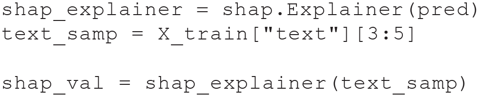
The SHAP values can be illustrated using the following code:

The color (blue or red) and color intensity in Figure 4 indicate how each word token affects the prediction of the text compared with the average prediction in the data set.

An illustration of SHAP values for the fourth and fifth texts in the training set, that is, the texts with Indices 3 and 4. Words shaded in blue decrease predicted contentment scores, and red words increase predicted contentment scores. The length of the arrows corresponds to their SHAP values. The base value represents the average prediction for observing high contentment (“Label 1”) in the training set. For the first example, the model predicts high contentment (“Label 1”), and for the second example, the model predicts low contentment (“Label 0”). SHAP = Shapley additive explanations.
We can interpret the plots in Figure 4 in the following way: Each plot displays the base value, which represents how often the given label is predicted on average across the entire training set. In this case, this base value is 0.51 for both instances. We also see the actual predictions for a high-contentment score for the two instances as numbers above the plots, which are close to 0.93 and 0.07. Therefore, the first instance, which is the fourth text of the training set, has a predicted value that is above average, and the second instance, which is the fifth text of the training set, has a prediction that is below average. The arrows in Figure 4 now aim to explain the differences between the observed prediction for each instance and the average prediction by contributing it to the word tokens in each instance. In the first instance, words like “dog” or the phrase “the weather is nice” lead to the prediction of a high-contentment score. In the second instance, words like “homework” lead to the prediction of a low-contentment score. Note that the sum of all SHAP values, which correspond to the lengths of the arrows, corresponds to the difference between the average prediction and the observed prediction for an instance.
LIME values
Similar to the computation of SHAP values, LIME values can be easily computed in Python. After installing the

Note that we also define the class names, which will be used in the following plots shown in Figure 5. As the next step, we need to define a prediction function, which again transforms a text into a set of probabilities. Because of technical requirements of the


An illustration of local interpretable model-agnostic explanation values highlighted for the fourth text of the training set.
Comparable with the

This leads to the output:

As before, we get a predicted probability of 0.85 for a low-contentment score and a predicted probability of 0.15 for a high-contentment score. We can now obtain an explainer that provides LIME values via
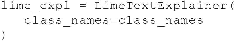
This function uses a lasso regression model as a surrogate model. We can now obtain LIME values for the fourth text via
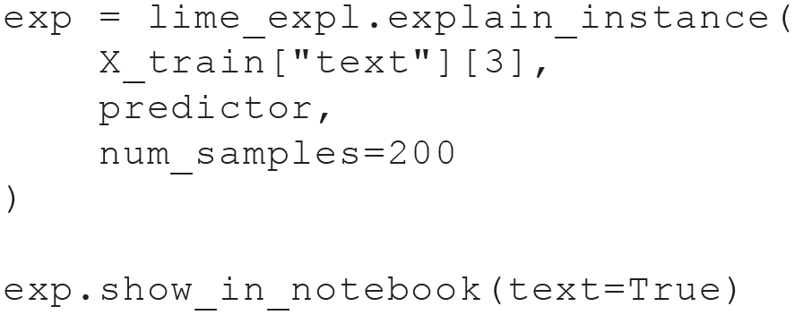
In the arguments, we set that we want to calculate our LIME values based on an artificial data set of 200 texts. This leads to the plot in Figure 5.
As for SHAP values, we receive graphical feedback on how single words affect predicted values. We again see the probabilities for high- and low-contentment scores in the upper left corner of Figure 5. Words like “dog” or “energy” increase the probability of a high-contentment score, and words like “homework” increase the probability of a low-contentment score. The numbers next to these words indicate how these probabilities would change after removing each word. For instance, removing “homework” would decrease the probability for a low-contentment score by 0.03. Thereby, IML methods, such as SHAP and LIME, can provide insights into how language use is associated with a psychological construct. In our case, we learn that students talking about dogs or the weather is usually predictive of them feeling content at the moment and that talking about homework is predictive of them being low in contentment.
Before concluding this section, we also discuss some current limitations of SHAP and LIME values, which are both conceptual and practical. They affect not only the presented implementations in Python but might also affect future implementations in other languages, such as R. First, LIME and SHAP values aim at clarifying relationships between the presence of work tokens and the prediction of an NLP model. They are therefore useful only if such a relationship can be established. Although this is the case in our example data, there might be cases in which such a relationship might be more opaque. Second, LIME values in particular are based on the interpretation of a substitute model and can therefore potentially be misleading. It is therefore important to supplement the interpretation of an NLP model by additional types of evidence, for instance, the prediction on benchmark data. Third, SHAP and LIME values can be computationally demanding, especially for large data sets and complex models.
Module 4 summary
To conclude this section, we summarize important differences between SHAP and LIME values. SHAP values are the only numerical representation of feature importance that exhibit the four mentioned characteristics of efficiency, symmetry, dummy, and additivity. From this perspective, SHAP values might be preferable for applications in psychology. LIME values, on the other hand, depend on a surrogate model, which is, by default, a lasso model in the
Conclusion and Outlook
In this tutorial, we have provided an end-to-end demonstration of how pretrained Transformer models can be used in text analysis with a focus on a use case in psychology. We specifically showed how Transformers can be used as feature extractors for subsequent ML models (e.g., in text classification). Alternatively, we demonstrated how to fine-tune a Transformer model for end-to-end classification of specific tasks to improve performance. Finally, we introduced two IML approaches (SHAP and LIME) for model interpretation.
LLMs are on a trajectory to become one of the most influential methodological advancements in the quantitative behavioral and social sciences. They are poised to revolutionize how research in these disciplines is conducted: Imminent applications include replacing standardized self-report questionnaires (Kjell et al., 2022), inferring psychological characteristics through text embeddings (Fan et al., 2023), and applying the Transformer architecture to other sequential data types (e.g., life records; Savcisens et al., 2024). In addition, LLMs can facilitate large-scale qualitative data analysis by automatically summarizing or coding open-ended responses of participants and generating new and psychometrically sound items (Krumm et al., 2024) or experimental vignettes. LLMs can even assist in theory building by helping researchers to rapidly synthesize theoretical or empirical work (Hermida Carrillo et al., 2024). In areas such as mental-health research, LLM-powered chatbots have the potential to provide scalable digital interventions while also generating new ethical and methodological considerations for clinical applications (Stade et al., 2024). Finally, there are many more use cases in psychology for which LLMs have the potential to exert a catalytic role. We anticipate seeing these models applied to computationally represent complex, context-dependent psychological phenomena in high-dimensional latent space (e.g., cognitive dissonance), train phenomenon-specific foundation models (e.g., for novel personality assessment), and generate data that are representative of psychological phenomena (e.g., text depressed people would produce; Vu et al., 2025). Finally, a shift in analysis methods will eventually also lead to more fundamental changes in the methodological curricula of students at universities (e.g., focus on NLP) and novel research practices (i.e., digitizing various aspects of human behavior), which could advance the field in the long term.
At the same time, LLMs are subject to limitations that require careful consideration when using these models for research (Feuerriegel et al., 2025). A primary concern is the lack of transparency regarding how these models generate responses and the specific data sets that were used for their training (Balloccu et al., 2024; Palmer et al., 2024). For example, the proprietary GPT-4.5 model’s specific training corpus remains unclear, as does the extent to which certain responses might be hard-coded (e.g., impossibility to produce critiques of certain people or institutions in the Grok model). Furthermore, the scale of resources required to train state-of-the-art LLMs is immense, with some relying on virtually the entire internet (e.g., Common Crawl) as their data source. The resulting high computational costs pose financial barriers and have a notable environmental impact (Strubell et al., 2019). Furthermore, LLMs can perpetuate existing biases in publicly available text, such as gender, age, or geographic stereotypes, because these models tend to replicate patterns found in their training data (Kotek et al., 2023; Manvi et al., 2024). Reproducibility of results can also be of concern because LLMs rely on probabilistic processes, such as random model initialization and stochastic sampling in text generation, which can make results difficult to replicate (Feuerriegel et al., 2025). Furthermore, older models or frameworks may quickly become obsolete. In addition, the underlying architectures, training data sets, and model parameters of LLMs are often not publicly available. This opacity prevents external validation or auditing, underscoring the importance of open, interpretable, and reproducible modeling approaches in research.
With these opportunities and challenges in mind, we hope that our tutorial will help behavioral scientists better understand and apply LLMs effectively in their research and thus advance the understanding of human psychology.
Supplemental Material
sj-pdf-1-amp-10.1177_25152459251351285 – Supplemental material for From Embeddings to Explainability: A Tutorial on Large-Language-Model-Based Text Analysis for Behavioral Scientists
Supplemental material, sj-pdf-1-amp-10.1177_25152459251351285 for From Embeddings to Explainability: A Tutorial on Large-Language-Model-Based Text Analysis for Behavioral Scientists by Rudolf Debelak, Timo K. Koch, Matthias Aßenmacher and Clemens Stachl in Advances in Methods and Practices in Psychological Science
Footnotes
Acknowledgements
We thank Samuel D. Gosling and Gabriella M. Harari for providing the data for the practical exercise and Felix Zimmer for giving feedback on a previous draft of this article.
Correction (October 2025):
Article updated to correct the OSF link on p. 7.
Transparency
Action Editor: Rogier Kievit
Editor: David A. Sbarra
Author Contributions
Notes
References
Supplementary Material
Please find the following supplemental material available below.
For Open Access articles published under a Creative Commons License, all supplemental material carries the same license as the article it is associated with.
For non-Open Access articles published, all supplemental material carries a non-exclusive license, and permission requests for re-use of supplemental material or any part of supplemental material shall be sent directly to the copyright owner as specified in the copyright notice associated with the article.