The Prior Odds of Testing a True Effect in Cognitive and Social Psychology

Abstract

Efforts to increase replication rates in psychology generally consist of recommended improvements to methodology, such as increasing sample sizes to increase power or using a lower alpha level. However, little attention has been paid to how the prior odds (R) that a tested effect is true can affect the probability that a significant result will be replicable. The lower R is, the less likely a published result will be replicable even if power is high. It follows that if R is lower in one set of studies than in another, then all else being equal, published results will be less replicable in the set with lower R. We illustrate this point by presenting an analysis of data from the social-psychology and cognitive-psychology studies that were included in the Open Science Collaboration’s (2015) replication project. We found that R was lower for the social-psychology studies than for the cognitive-psychology studies, which might explain why the rate of successful replications differed between these two sets of studies. This difference in replication rates may reflect the degree to which scientists in the two fields value risky but potentially groundbreaking (i.e., low-R) research. Critically, high-R research is not inherently better or worse than low-R research for advancing knowledge. However, if they wish to achieve replication rates comparable to those of high-R fields (a judgment call), researchers in low-R fields would need to use an especially low alpha level, conduct experiments that have especially high power, or both.

In years gone by, it was often assumed that if a low-powered (e.g., small-n) experiment yielded a significant result, then not only was the effect probably real, but its effect size was probably large as well. After all, how would the effect have been detected if that were not the case? If anything, low-powered studies finding significant effects once seemed like a good thing, not a bad thing. In recent years, however, it has become apparent that there is a problem with this line of thinking. As it turns out, if researchers in a field typically run low-powered experiments, the significant effects reported in the field’s scientific journals will often be false positives, not real effects with large effect sizes (Button et al., 2013).

The probability that a significant effect is real is known as the positive predictive value (PPV). Button et al. (2013) pointed out that the equation specifying the relationship between PPV and power is as follows:

$$PPV=\left[\left(1-\beta \right)\times R\right]/\left[\left(1-\beta \right)\times R+\alpha \right],$$

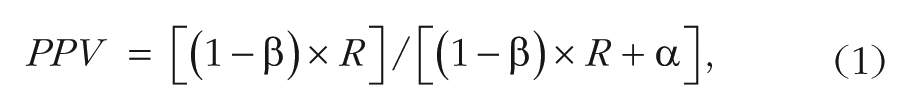
where 1 − β represents power, α represents the Type I error rate (usually .05), and R represents the prestudy odds that real effects are investigated in the scientific field in question. The main focus of this article is the potential importance of R—that is, the potential importance of the base rate of tested effects with nonzero effect sizes among the totality of effects subjected to empirical investigation in a given scientific field.

Button et al. (2013) showed that a significant effect is more likely to be real if it was obtained with a high-powered study than if it was obtained with a low-powered study. All else being equal, if field A runs high-powered studies and field B runs low-powered studies, then significant effects from field A will be more replicable than significant effects from field B will be, which is to say that PPV will be higher for field A than for field B. In their calculations, Button et al. held R constant to illustrate the point that power affects PPV. However, other researchers have noted the importance of differing prior odds (e.g., Lakens & Evers, 2014; Overall, 1969).

R Matters, Too

In medicine, it is well known that base rates play a critical role in the likelihood of a positive test result actually indicating a true positive result (Gigerenzer, 2015; Hoffrage & Gigerenzer, 1998). Consider a disease so rare that for every 1 person who has the disease, 100,000 do not, and assume a test so diagnostic of the disease that it is correct 99.99% of the time (i.e., true positive rate = .9999, false positive rate = .0001). What are the odds that a person who tests positive actually has the disease? The answer is provided by Bayes rule, which, in odds form, is given by

$$\mathrm{posterior\; odds}=\mathrm{prior\; odds}\times \mathrm{likelihood\; ratio}.$$

In this example, the prior odds are 1/100,000, and the likelihood ratio is the true positive rate divided by the false positive rate, or .9999/.0001. Multiplying the prior odds by the likelihood ratio yields a posterior odds of approximately .1. In other words, despite the test being incredibly diagnostic, a positive test result means that there is only a 1-in-10 chance that the tested person actually has the disease. Expressed as a probability, the PPV in this case can be calculated as follows: PPV = posterior odds/(posterior odds + 1) = .1/(.1 + 1) = .09.

What if, instead, there is an a priori reason to believe that the next tested individual has this rare disease, because he or she is already showing signs of it (e.g., a distinctive skin-coloring pattern)? Imagine that prior research has shown that among people with that symptom, the odds of having the disease are 50/50. Under these conditions, the prior odds are even, in which case Bayes rule indicates that a positive test result means the posterior odds that the individual has the disease are 9,999 to 1 (i.e., PPV = .9999).

This example illustrates the fact that when there is a good reason to believe that someone actually has the disease before the test is run, a positive test result can strongly imply that the person has the disease (PPV is high). By contrast, when there is no reason to believe that someone actually has the disease before the test is run, a positive test result—even from a highly diagnostic test—may strongly imply that a person does not have the disease (PPV is low). Although such a test will update the prior odds from being extremely low to being much higher than they were before, the posterior odds (and PPV) can still weigh heavily against the disease being present.

Just as the prior odds that someone has a disease affect the meaning of a positive test, the prior odds that an experiment is testing a true effect (i.e., R) should influence one’s belief in that effect following a significant result. In the example just described, even an extremely diagnostic test did not strongly imply a true positive result when the test was run without any prior reason for conducting the test in the first place. As strong as the research methodology in psychology may be, no one would argue that psychology experiments are anywhere near 99.99% diagnostic of a true effect (i.e., that they correctly detect true effects 99.99% of the time and generate false positives 0.01% of the time). It is therefore important to consider the factors that determine which specific hypotheses among the entire population of hypotheses scientists choose to test when they conduct an experiment. The fewer advance signs that the effect might be true, the lower R is likely to be (just as in our example of the rare disease).

R May Differ Across Types of Studies

To investigate the potential role of R, we compared two sets of studies from different subfields of experimental psychology—cognitive psychology and social psychology—that the Open Science Collaboration (2015) found to have different rates of successful replication (and, therefore, different PPVs). In this project, researchers conducted replications of 100 quasirandomly sampled studies published in three psychology journals. Of the 100 replicated studies, 57 were from social psychology and 43 were from cognitive psychology. ¹ The Open Science Collaboration reported that 50% of the findings in cognitive psychology and 25% of the findings in social psychology were replicated at the p < .05 level. This difference in replication rates was significant, z = 2.49, p = .013. It is likely that the percentage of the originally reported effects that were real is larger than what the project indicated because not every real effect will be detected when studies are replicated, and the miss rate likely exceeds the false-positive rate. One way to estimate how many of the effects were real is to consider the proportion that were replicated (regardless of the p value) in the same direction as originally observed. This proportion was significantly higher for cognitive psychology (.905) than for social psychology (.745), z = 2.00, p = .046. Because this was a study with a relatively small sample, it seems fair to say that this statistical comparison does not provide strong evidence for a true difference between the two subfields. Nevertheless, we use these point estimates to illustrate how R might help to account for the differing replication rates of the cognitive- and social-psychology studies included in the Open Science Collaboration’s project.

Using binary logic for the time being, we assume that the observed proportion of studies yielding effects in the same direction as originally observed, ω, is equal to the proportion of true effects, PPV, plus half of the remaining 1 – PPV noneffects, which would be expected to yield effects in the same direction as originally observed 50% of the time by chance. The mathematical equation can be expressed as follows: ω ≈ PPV + .50(1 – PPV). Thus, PPV is approximately 2ω – 1 (see Box 1 for more details). For cognitive psychology, ω = .905, so the PPV for cognitive psychology is 2(.905) – 1, or .81. For social psychology, ω = .745, so the PPV for social psychology is 2(.745) – 1, or .49. In other words, using this measure, 81% of the originally reported cognitive-psychology effects were real, whereas only 49% of the originally reported social-psychology effects were real. What is the reason for the difference?

Box 1.

Calculating the Positive Predictive Value (PPV)

PPV can be estimated by understanding the probability of different outcomes. Consider a null hypothesis, H₀, that the effect of interest is not real. The top panel of Figure 1 shows how a test statistic (e.g., Student’s t) will be distributed if the null hypothesis is true. This distribution is centered on zero because any observed effects (e.g., t values different from zero) are due purely to noise. Half of the time, effects observed when H₀ is true will be positive, and the other half of the time, effects observed when H₀ is true will be negative. The areas shaded in the upper and lower tails of this distribution represent the Type I error rate (α = .05). Now consider an alternative hypothesis, H₁, that the effect of interest is real. The bottom panel of Figure 1 shows how a test statistic will be distributed if this alternative hypothesis is true; one distribution is for experiments with 50% power, and the other is for experiments with 80% power (i.e., either 50% or 80% of the distribution, respectively, exceeds the critical value of the test statistic). If a replication experiment has 50% power, the probability of a real effect going in the direction opposite the true effect (denoted as δ) is approximately .02. If a replication experiment instead has 80% power, δ is approximately .003 (a probability so small that it is hard to see in the figure). Thus, the full equation for ω is as follows: ω = (1 – δ)PPV + .5(1 – PPV). Solving for PPV shows that it is equal to (ω – .5)/(.5 – δ). Because δ is likely negligible for the replication studies in our analysis, we rely on the simpler equation, PPV = 2ω − 1, as a close approximation. Johnson, Payne, Wang, Asher, and Mandal (2017) used a different approach to estimate PPV for a subset of the Open Science Collaboration’s (2015) replication studies and obtained an estimate similar to the one we obtained using our simple equation (see the Supplemental Material available online for more details).

Fig. 1.

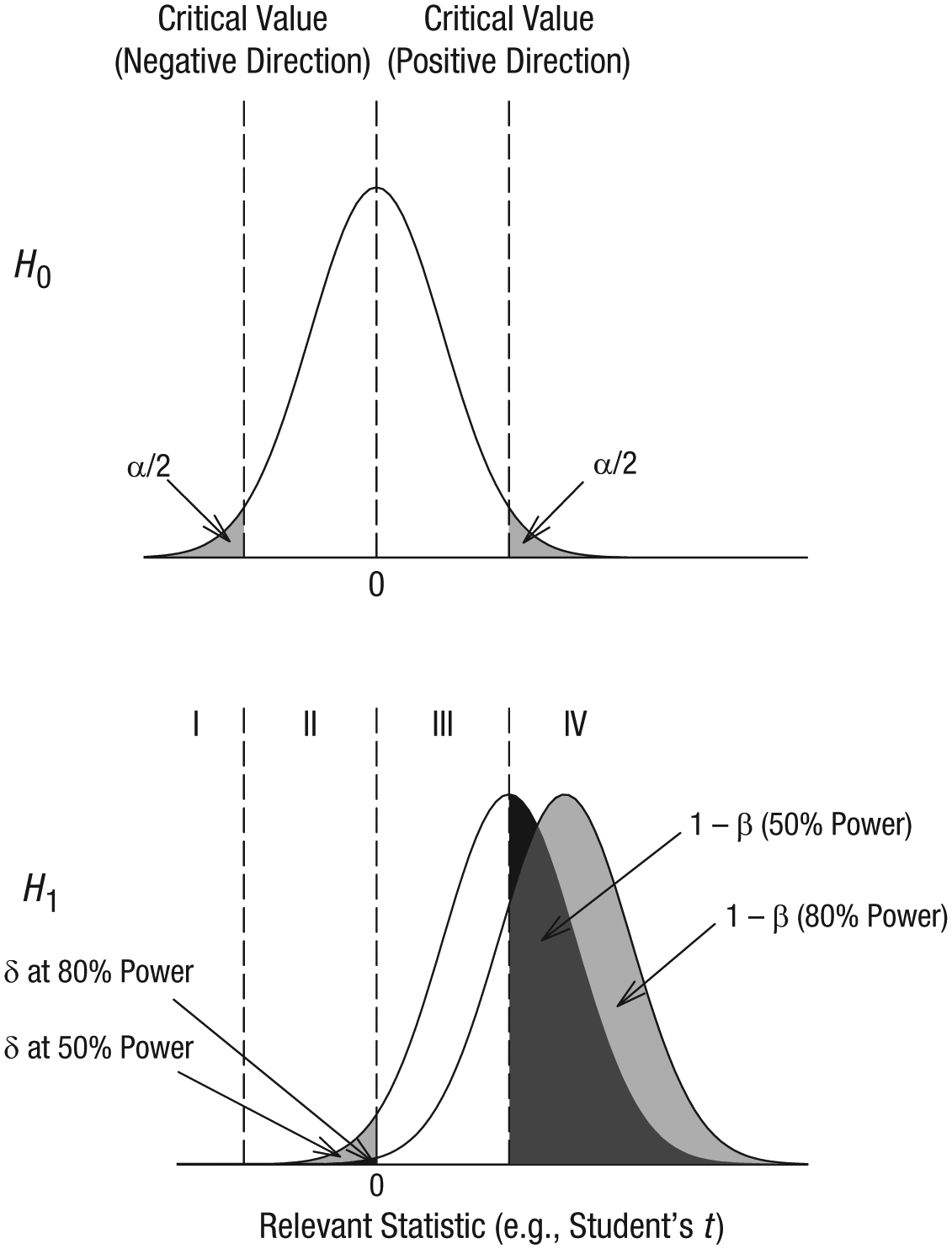
Test-statistic distributions obtained when the effect of interest is not real (H₀; top panel) and when it is real (H₁; bottom panel). For effects that are real, the graph shows a distribution for experiments with 50% power and a distribution for experiments with 80% power.

For H₁, the area in Region I corresponds to the probability of observing a significant effect in the wrong direction if the effect is real. Clearly, it is extremely unlikely that a significant result is in the wrong direction even if the study had power as low as 50%. Indeed, Gelman and Carlin (2014) showed that this kind of error (which they termed a Type S error) becomes appreciable only when power drops well below 20%. We assume that the original studies in the Open Science Collaboration’s (2015) project did not have power well below 20%. If that assumption is correct, then significant Type S errors can be ignored in our analyses without appreciably affecting our estimates of PPV. The area in Region II corresponds to the probability of observing a nonsignificant effect in the wrong direction if an effect is real. The area in Region III corresponds to the probability of getting a nonsignificant result in the correct direction if an effect is real, and the area in Region IV corresponds to the probability of getting a significant result in the correct direction if an effect is real.

As noted in the Open Science Collaboration’s (2015) article, “reproducibility may vary by subdiscipline in psychology because of differing practices. For example, within-subjects designs are more common in cognitive than social psychology, and these designs often have greater power to detect effects with the same number of participants” (p. aac4716-2). The authors focused on experimental-design issues (and resulting differences in statistical power) to explain the difference in reproducibility rates between cognitive- and social-psychology studies. Such an interpretation carries with it the implication that R is the same for both sets of studies and that increasing statistical power in social psychology would have resulted in replication rates comparable to those in cognitive psychology. We next consider whether a difference in statistical power between the two groups of studies included in the Open Science Collaboration’s project is sufficient to explain the difference between their PPVs or whether a difference in R—the odds that the tested effects were real—is also needed to explain that difference. In this analysis, we treat the point estimates from the project as being the true values even though there is likely to be error in those estimates.

Can a Difference in Power Explain the Difference in PPV?

According to Equation 1, PPV is affected by three variables: power (1 − β); base rate, or prior odds (R); and alpha level. Social and cognitive psychology generally follow the same convention for their alpha level (i.e., p < .05), so the difference in that variable likely does not explain the difference in PPV. This leaves two other variables that might explain differences in the percentage of claimed discoveries that actually are true: power and base rate of true effects. If either (or both) of these variables is lower in social than in cognitive psychology, the percentage of claimed discoveries that are actually true (PPV) would also be lower in social psychology. The usual assumption is that studies in social psychology are underpowered compared with studies in cognitive psychology, and that this explains the lower replication rate. As we discussed earlier, Equation 1 predicts that low power alone is theoretically sufficient to have that effect. However, another possibility is that the cognitive- and social-psychology studies in the Open Science Collaboration’s (2015) sample differed in R, not power.

Assume for the sake of argument that power was actually the same for the two sets of studies and that it was equal to 80%. With power specified at 80% and α set to .05 for both sets of studies, and with PPV set to .49 for the social-psychology studies and to .81 for the cognitive-psychology studies (on the basis of the analysis presented earlier), one can use Equation 1 to solve for R, separately for the two sets of studies. Rearranged to solve for R, Equation 1 becomes

$$R=\alpha PPV/\left[\left(1-\beta \right)\times \left(1-PPV\right)\right].$$

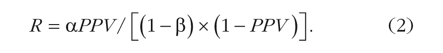
Equation 2 yields R estimates of .27 for cognitive psychology and .06 for social psychology. The corresponding probabilities, R/(R + 1), come to .21 and .06, respectively. That is, if these point estimates from the Open Science Collaboration’s (2015) project are representative of the field at large, then in cognitive psychology, for every real effect that is subjected to empirical test, there are about 4 noneffects that are subjected to empirical test. For social psychology, for every real effect that is subjected to empirical test, there are about 16 noneffects that are subjected to empirical test. Keep in mind that these estimates of R pertain to the number of true effects out of the totality of effects that are subjected to empirical investigation (i.e., prior odds), not to the number of true effects in the published literature out of the totality of published effects (i.e., not to posterior odds or to PPV).

Although we equated power at 80% in this example, the underlying base rate of true effects would be lower for the social-psychology studies than for the cognitive-psychology studies for any level of (equated) power we might choose. Thus, although the observed difference in replication rates for the cognitive- and social-psychology studies can be accounted for by assuming that the original studies differed in power (which is the usual assumption), those differences can also be accounted for by assuming that the studies were equal in power but differed in the probability of true effects tested.

How can one determine whether one of these explanations (i.e., differential power or differential R) actually accounts for the observed difference in the replication rates or whether both explanations account for this difference? Some insight into the question of whether or not the originally published cognitive- and social-psychology studies differed in power can be obtained by examining the p-curves for the two sets of studies. Simonsohn, Nelson, and Simmons (2014) performed simulations for various levels of power and showed what the distributions of p values look like for 50% and 80% power. The distributions are right skewed in both cases, but as power increases, the proportion of significant p values less than .01 increases. In these simulations, with 50% power, about 50% of the significant p values were less than .01. With 80% power, about 70% of the significant p values were less than .01. Simonsohn et al. found that these patterns held true for a wide range of effect sizes and sample sizes. Thus, for example, for 50% power, the p-curve when Cohen’s d was 0.64 and n was 20 was similar to the p-curve when Cohen’s d was 0.28 and n was 100. Moreover, in an online supplement (Supplement 2), Simonsohn et al. concluded that p-curve is robust to heterogeneity of effect size. Although other researchers disagree with that claim (Schimmack & Brunner, 2017) and the issue remains unresolved, we used p-curves to obtain tentative estimates of power for illustrative purposes.

Figure 2 shows the p-curves (distributions of significant p values) for the original cognitive- and social-psychology studies included in the Open Science Collaboration’s (2015) sample. These p-curves are consistent with the widely held view that social-psychology studies have lower power than cognitive-psychology studies. More specifically, the p-curve for the original cognitive-psychology studies resembles the hypothetical p-curves associated with 80% power in Figure 1 of Simonsohn et al. (2014). The p-curve for the original social-psychology studies resembles the hypothetical p-curves associated with 50% power in Simonsohn et al.’s figure. Whether or not these exact power estimates are correct, the p-curve data are consistent with the prevailing view that power was lower in the original social-psychology studies than in the original cognitive-psychology studies.

Fig. 2.

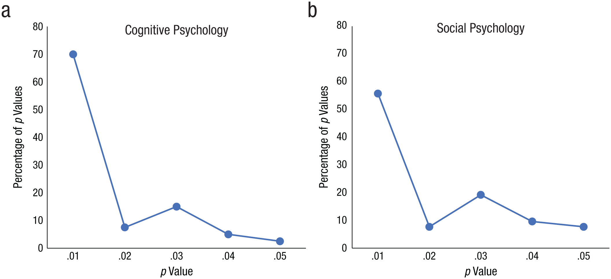
Distributions of p values for studies replicated in the Open Science Collaboration’s (2015) project: (a) the p values from the original cognitive-psychology studies and (b) the p values from the original social-psychology studies.

Although a difference in power may provide part of the explanation for the difference in replication rates between the two sets of studies, it does not seem to explain the entire difference. If we set PPV to .49, α to .05, and 1 – β (i.e., power) to .50 for the social-psychology studies and we set the corresponding values to .81, .05, and .80 for the cognitive-psychology studies, Equation 2 shows that R is .10 (odds = 1 to 10) for social psychology and .27 (odds = 1 to ~4) for cognitive psychology. In other words, according to this analysis, even allowing for the fact that the cognitive- and social-psychology studies differed substantially in statistical power (50% for social psychology vs. 80% for cognitive psychology in this example), they also differed in the likelihood that a tested effect was real. This analysis is based on simplified binary logic (according to which effect sizes are real or not) and assumes that these point estimates for R and power are the true values. However, a more realistic assumption is that effect sizes are continuously distributed (see Box 2). Even assuming continuous effect-size distributions, if we define a real effect as one that exceeds a certain criterion (e.g., d > 0.1), PPV was higher for cognitive than for social psychology (see the appendix).

Box 2.

Effect Sizes Are Continuously Distributed

The analysis presented in the main text is based on binary logic (i.e., it assumes that effects are either real or not), which is a convenient assumption for thinking through these issues but is also unrealistic. Undoubtedly, effect sizes have continuous distributions, beginning with an effect size of zero and increasing in continuous fashion to effect sizes that are much greater than zero. Thus, for example, if one assumes that some hypotheses have effect sizes of 0, it seems odd to suppose that there are not other hypotheses with effect sizes of 0.001, still others with effect sizes of 0.002, and so on.

In some fields of research, such as in genomewide-association studies (e.g., Park et al., 2010), there are theoretical reasons to believe that effect sizes are exponentially distributed. If effect sizes happen to be exponentially distributed in psychology, then empirical effect sizes, which are measured with Gaussian error, should have an ex-Gaussian distribution. To examine this possibility, we looked to Szucs and Ioannidis’s (2017) analysis of the distribution of published effect sizes from 3,801 recently published articles in psychology and cognitive neuroscience. From that data set, we selected the significant effect sizes in psychology that had Cohen’s d values less than 5.0 (a very small percentage of effects were larger). Figure 3 shows the distribution of those effect sizes. The curve shows the maximum likelihood fit of the three-parameter ex-Gaussian distribution, which appears to provide a reasonable approximation to the large majority of the effect sizes. The mean of the exponential distribution is represented by τ, and the mean and standard deviation of the Gaussian component are µ and σ, respectively. The overall average effect size is equal to µ + τ, which is 0.96 (0.28 + 0.68) for these data. Because these are maximum likelihood estimates, the estimated average effect size of 0.96 is the same value one obtains by simply averaging the 5,334 effect sizes in the sample. See the appendix for how this approach can be used to analyze the Open Science Collaboration’s (2015) data.

Fig. 3.

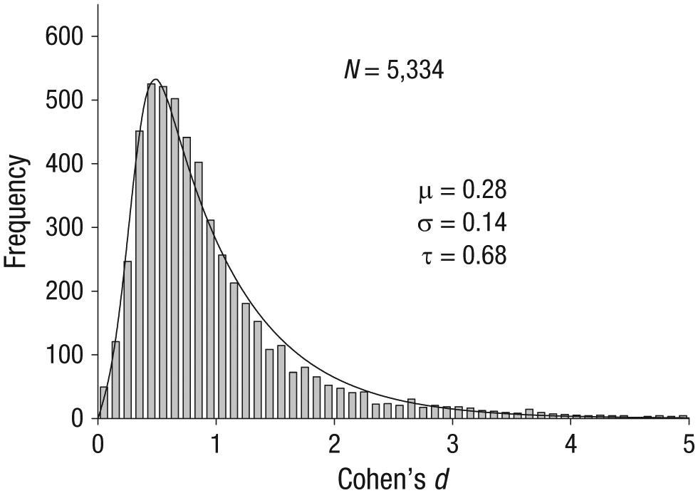
Maximum likelihood fit of the ex-Gaussian distribution to the significant effect sizes taken from Szucs and Ioannidis’s (2017) data set.

An alternative way of making this same point is to assume that R was actually the same for the cognitive- and social-psychology studies and then to consider just how much lower the power of the social-psychology studies would have had to have been for the two sets of studies to yield PPV values of .81 and .49, respectively. For this analysis, we rearrange Equation 1 again, this time solving for power:

$$(1-\beta )=\alpha PPV/[R\times (1-PPV)].$$

We set PPV in Equation 3 to .81 for the cognitive-psychology studies and to .49 for the social-psychology studies; alpha is set to .05 for both sets of studies. For a given value of R (which is constrained to be equal for cognitive and social psychology), we can then estimate power. For example, if R is .266, then Equation 3 indicates that power for the cognitive-psychology studies was .80, whereas power for the social-psychology studies was only .18. Did the power of the two sets of studies actually differ to that great an extent? Perhaps, but then one would need to explain why the p-curve for social psychology (in Fig. 2) is closer to the 50%-power p-curve than the 25%-power p-curve in Simonsohn et al.’s (2014) simulations.

Figure 4a shows a generalization of this example. More specifically, the figure shows what statistical power for the social-psychology studies would have had to have been for any level of power in the cognitive-psychology studies under the assumption that the underlying base rates were the same in the two sets of studies. For example, according to Equation 3, if the cognitive-psychology studies had 100% power (i.e., if R = .213), power for the social-psychology studies would have had to have been only 23%. In other words, 23% is the maximum power that the social-psychology studies could have had if the two sets of studies were equated with respect to R. As far as we can tell, no one has argued (and the p-curve analysis does not suggest) that the power differential between the cognitive- and social-psychology studies was that extreme. Instead, it seems more reasonable to assume that although the power of the two sets of studies may have differed, R differed as well. Similarly, Figure 4b shows that R would have had to have been vastly lower for the social-psychology studies than for the cognitive-psychology studies in order for the two sets of studies to have been equated with respect to power. Given the large differences in power or R that one would otherwise have to assume, it seems reasonable to assume that both factors (lower power and lower R) played a role in the lower rate of replication observed for social psychology. We cannot conclusively state that the differences in R between cognitive and social psychology that were observed in the Open Science Collaboration’s (2015) data set will generalize more broadly to those subfields of psychology, but it seems reasonable to suppose that they might.

Fig. 4.

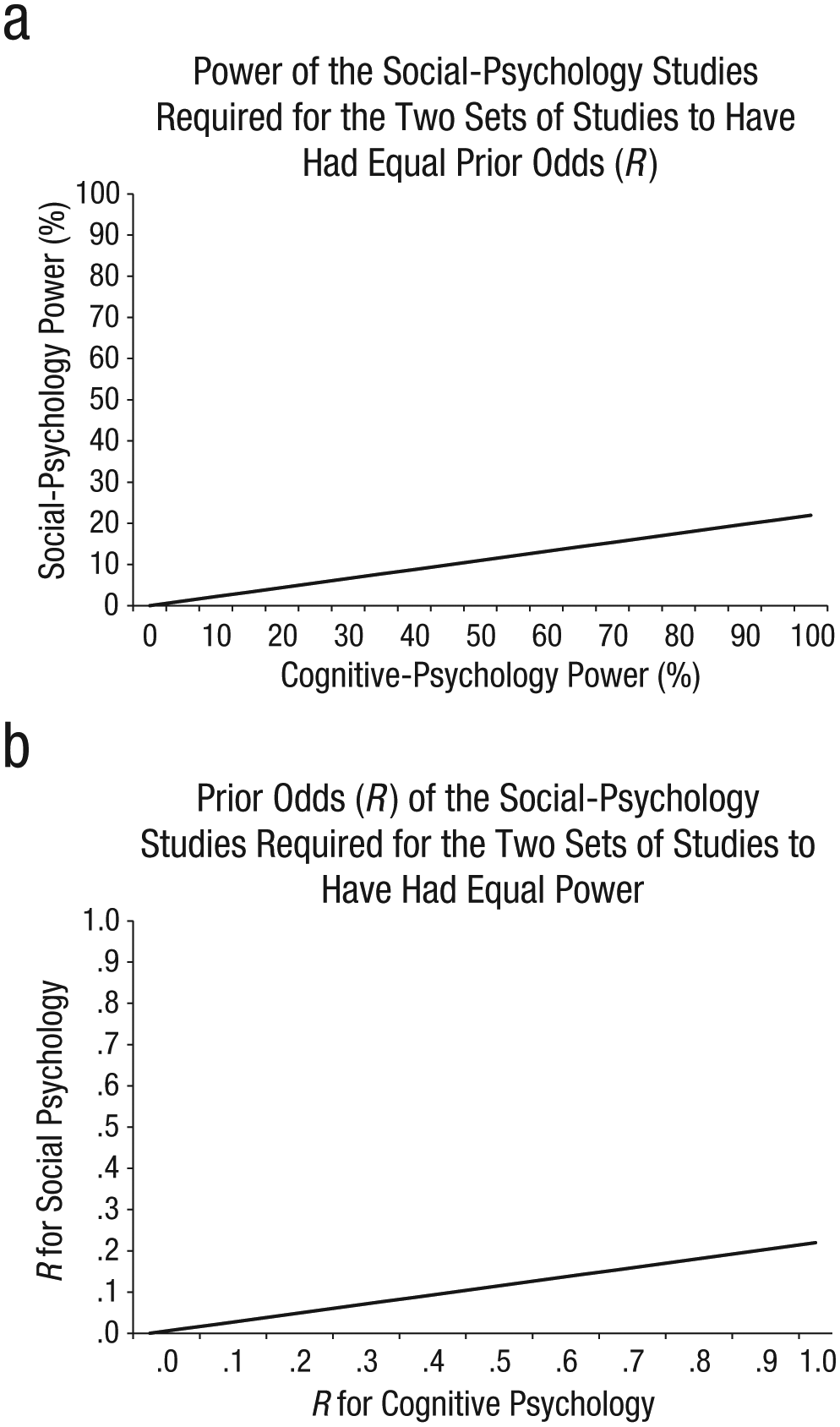
Illustration of differences in power and differences in the base rate of true effects (R) that would be required for either of these factors by itself to account for the lower rate of successful replication for the social-psychology studies compared with the cognitive-psychology studies in the Open Science Collaboration’s (2015) replication project. The graph in (a) shows how much lower the power in the social-psychology studies would have had to have been compared with the power of the cognitive-psychology studies in order for the prior odds of studying true effects to have been equal for the two sets of studies. The graph in (b) shows how much lower the prior odds of studying true effects would have had to have been in the social-psychology studies relative to the cognitive-psychology studies for the power of the two sets of studies to have been equal.

Factors Affecting R

What factors determine the prior odds that a tested hypothesis is true? Our assumption is that established knowledge is the key consideration, just as it is in the medical domain when one is considering the prior odds that an individual has a particular disease. Experiments that test hypotheses based on established knowledge, acquired either from scientific research or from common experience (e.g., going without sleep makes a person tired), have higher Rs compared with experiments that test hypotheses relying on less dependable sources of knowledge, such as hunches or theories grounded in scientists’ idiosyncratic personal experiences.

We illustrate this point with an extreme example of low-R research. Imagine that you are walking around the grocery store one afternoon and eye some balloons on your way to the checkout line. You decide to buy them and randomly place them outside the doors of some classrooms and not others, to test a novel theory that doing so will boost morale and help to address the problem of scholastic underachievement. This theory might be based on your own childhood experiences with the effect of ambient balloons on your motivation to excel in math. You then measure students’ learning in the classrooms with and without balloons at their doors. Suppose you even get a statistically significant difference (p < .05) between the learning scores in the two conditions. The danger with relying on these surprising results and starting your new Balloon Brain business designed to harness the power of balloons in classrooms is that the prior odds of your hypothesis being true are low because of the way that the balloon idea was generated (i.e., the idea was largely untethered to established knowledge).

The results of low-R research will be more surprising than the results of high-R research because, by definition, a result is surprising to the extent that it violates one’s priors. In the medical context, for example, if someone who is already showing signs of a rare disease (high prior odds) tests positive, that outcome would probably not be viewed as very surprising. By contrast, if someone who is showing no signs of a rare disease (low prior odds) nevertheless tests positive, that outcome probably would be viewed as surprising. Conceivably, social psychologists place higher value on surprising findings—that is, findings that reflect a departure from what is already known—than cognitive psychologists do (e.g., editors of social-psychology journals might place greater weight on the surprisingness factor). All else being equal, a difference in preference along that dimension would lead to a difference in R between the two fields (i.e., lower R for social psychology). In agreement with this line of reasoning, the Open Science Collaboration (2015) asked independent coders to rate how surprising and how exciting or important the findings reported in the original studies in the sample were. ² When these two measures were averaged together, the original cognitive-psychology studies were rated as being less surprising and exciting (M = 3.04 out of 6) than the original social-psychology studies (M = 3.33), t(110) = −2.25, p = .026.

A difference in preference for more surprising versus less surprising findings would not be an automatic indictment of either field. Indeed, there is an inherent tension between the degree to which a study will advance knowledge and the likelihood that a reported effect is replicable. Researchers in different fields may have different preferences for where they would like to operate on the R continuum. If R for a particular field were 0, the published literature would likely be very exciting to read (i.e., it would provide large apparent leaps in knowledge, such as findings that people have ESP), but none of it would be true. At the other extreme, if R for a particular field were infinitely high, the published literature would all be true, but the results of most experiments might be so preexperimentally obvious as to be useless. Maximizing PPV solely by maximizing R would serve only to “enshrine trivial, safe science” (Mayo & Morey, 2017, p. 26). We can imagine pages full of findings that people are hungry after missing a meal or that people are sleepy after staying up all night. Neither of these scenarios (R = 0 or R = ∞) would be ideal for advancing understanding of the world. The ideal point on the R continuum lies somewhere in between, but specifying the optimal point is difficult (see Miller & Ulrich, 2016) even though increasing R increases replicability.

Implications

In response to concerns regarding replication rates in experimental psychology, researchers have made many methodological recommendations, but they have focused on factors that affect power rather than R. For example, Psychological Science now asks submitting authors “to explain why they believe that the sample sizes in the studies they report were appropriate” (Association for Psychological Science, 2017, Research Disclosure Statements). The Attitudes and Social Cognition section of the Journal of Personality and Social Psychology now requires authors to include “a broad discussion on how the authors sought to maximize power” (American Psychological Association, 2017). Psychonomic Bulletin & Review now instructs submitting authors that “it is important to address the issue of statistical power. . . . Studies with low statistical power produce inherently ambiguous results because they often fail to replicate” (Psychonomic Society, 2017, Instructions for Authors: Statistical Guidelines, paragraph 2). Equation 1 makes it clear why that is the case, but power is not the only factor that will affect replication rates. ³

In addition to a growing understanding of the importance of power, there is an increasing awareness of how the alpha level affects the likelihood of a false positive. For example, Lindsay (2015) suggested that findings with a p value just barely below .05 should be regarded with more skepticism than is typically the case. Along the same lines, Benjamin et al. (2018) recently proposed that the standard for statistical significance for claims of new discoveries should be p < .005 rather than p < .05 in order to make published findings more replicable. These developments underscore the fact that, in addition to running studies with higher power, lowering the alpha level will increase PPV (Equation 1).

If our analysis is correct, then neither of these approaches, if applied nondifferentially, would do away with the difference in replicability between the cognitive- and social-psychology studies we analyzed. If R differed between the two sets of studies, then even if power were set to 80% and alpha were set to .005, the effects observed in the cognitive-psychology studies would still be more likely to be replicable than those observed in the social-psychology studies. Given our prior estimate of R for the cognitive-psychology studies, Equation 1 indicates that these standards would result in 97.7% of published cognitive-psychology effects being true. For the social-psychology studies, 90.6% would be true (a result that could be achieved in cognitive psychology using an alpha level of .022). Therefore, if researchers in a given field prefer to engage in risky (low-R) research, either higher power or a lower alpha (or some combination of the two) would be needed in order for them to achieve the same PPV as in a field with less risky research.

If, instead, the same methodological standards are applied to both fields (e.g., 80% power and alpha of .005), and if researchers in the two fields prefer to have the same high PPV (a judgment call), then researchers in the low-R discipline would need to increase R. One way to increase R would be to base new experiments more directly on knowledge derived from prior scientific research rather than test hypotheses farther away from what is scientifically known. Such a change in focus would presumably happen only if editors of top journals in the high-risk (low-R) field placed slightly less emphasis than they usually do on the novelty of new findings (in which case, scientists themselves might do the same). Low-R research is likely to be surprising and exciting, but unless it has differentially high power or a differentially low alpha level, it is likely to be less replicable than high-R research.

Supplemental Material

WilsonOpenPracticesDisclosure – Supplemental material for The Prior Odds of Testing a True Effect in Cognitive and Social Psychology

Supplemental material, WilsonOpenPracticesDisclosure for The Prior Odds of Testing a True Effect in Cognitive and Social Psychology by Brent M. Wilson and John T. Wixted in Advances in Methods and Practices in Psychological Science

Supplemental Material

WilsonSupplementalMaterial – Supplemental material for The Prior Odds of Testing a True Effect in Cognitive and Social Psychology

Supplemental material, WilsonSupplementalMaterial for The Prior Odds of Testing a True Effect in Cognitive and Social Psychology by Brent M. Wilson and John T. Wixted in Advances in Methods and Practices in Psychological Science