
Abstract
We conducted preregistered replications of 28 classic and contemporary published findings, with protocols that were peer reviewed in advance, to examine variation in effect magnitudes across samples and settings. Each protocol was administered to approximately half of 125 samples that comprised 15,305 participants from 36 countries and territories. Using the conventional criterion of statistical significance (p < .05), we found that 15 (54%) of the replications provided evidence of a statistically significant effect in the same direction as the original finding. With a strict significance criterion (p < .0001), 14 (50%) of the replications still provided such evidence, a reflection of the extremely high-powered design. Seven (25%) of the replications yielded effect sizes larger than the original ones, and 21 (75%) yielded effect sizes smaller than the original ones. The median comparable Cohen’s ds were 0.60 for the original findings and 0.15 for the replications. The effect sizes were small (< 0.20) in 16 of the replications (57%), and 9 effects (32%) were in the direction opposite the direction of the original effect. Across settings, the Q statistic indicated significant heterogeneity in 11 (39%) of the replication effects, and most of those were among the findings with the largest overall effect sizes; only 1 effect that was near zero in the aggregate showed significant heterogeneity according to this measure. Only 1 effect had a tau value greater than .20, an indication of moderate heterogeneity. Eight others had tau values near or slightly above .10, an indication of slight heterogeneity. Moderation tests indicated that very little heterogeneity was attributable to the order in which the tasks were performed or whether the tasks were administered in lab versus online. Exploratory comparisons revealed little heterogeneity between Western, educated, industrialized, rich, and democratic (WEIRD) cultures and less WEIRD cultures (i.e., cultures with relatively high and low WEIRDness scores, respectively). Cumulatively, variability in the observed effect sizes was attributable more to the effect being studied than to the sample or setting in which it was studied.
Keywords
Suppose a researcher, Josh, conducts an experiment and finds that academic performance is reduced among participants who experience threat compared with those in a control condition. Another researcher, Nina, conducts the same study at her institution and finds no effect. Person- and situation-based explanations of the discrepancy may come to mind immediately: Nina may have used a sample that differed in important ways from Josh’s sample, and the situational context in Nina’s lab might have differed in theoretically important but nonobvious ways from the context in Josh’s lab. Both explanations could be true. A less interesting, but real, possibility is that one of the researchers made an error in design or procedure that the other did not. Finally, it is possible that the different results are a function of sampling error: Nina’s result could be a false negative, or Josh’s result could be a false positive. The present research provides evidence toward understanding the contribution of variation in samples and settings to observed variation in psychological effects.
Accounting for Variation in Effects: Person and Situation Variation, or Sampling Error?
There is a body of research providing evidence that experimental effects are influenced by variation in person characteristics and experimental context (Lewin, 1936; Ross & Nisbett, 1991). For example, people tend to attribute behavior to characteristics of the person rather than characteristics of the situation (e.g., Gilbert & Malone, 1995; Jones & Harris, 1967), but some evidence suggests that this effect is stronger in Western than in Eastern cultures (Miyamoto & Kitayama, 2002). A common model of investigating psychological processes is to identify an effect and then investigate moderating influences that make the effect stronger or weaker. Therefore, when similar experiments yield different outcomes, the readily available conclusion is that a moderating influence accounts for the difference. However, if effects vary less across samples and settings than is assumed in the psychological literature, then the assumptions of moderation may be overapplied and the role of sampling error may be underestimated.
If effects are highly variable across samples and settings, then variation in effect sizes will routinely exceed what would be expected to result from sampling error. In this circumstance, the lack of consistency between Josh’s and Nina’s results is unlikely to influence beliefs about the original effect. Moreover, if there are many influential factors, then it is difficult to isolate moderators and identify the conditions necessary to obtain the effect. In this case, the lack of consistency between Josh’s and Nina’s results might produce collective indifference—there are just too many variables to know why there was a difference, so the different results produce no change in understanding of the phenomenon.
Alternatively, variations in effect sizes may not exceed what would be expected to result from sampling error. In this case, observed differences in effects do not indicate moderating influences of sample or setting. Rather, imprecision in estimation is the sole source of variation and requires no causal explanation.
In the case of Josh’s and Nina’s results, it is not necessarily easy to assess whether the inconsistency is due to sampling error or moderation, especially if their studies had small samples (Morey & Lakens, 2016). With small samples, Josh’s positive result and Nina’s null result will likely have confidence intervals that overlap each other, so that one can conclude little other than that “more data are needed.”
The difference between these interpretations regarding the source of the inconsistency is substantial, but there is little direct evidence regarding the extent to which persons and situations—samples and settings—influence the size of psychological effects in general (but see Coppock, in press; Krupnikov & Levine, 2014; Mullinix, Leeper, Druckman, & Freese, 2015). The default assumption is that psychological effects are awash in interactions among many variables. The present report follows up on initial evidence from the Many Labs projects (Ebersole et al., 2016; Klein et al., 2014a). The first Many Labs project (Klein et al., 2014a) replicated 13 classic and contemporary psychological effects with 36 different samples and settings (N = 6,344). The results showed that (a) variation in sample and setting had little impact on observed effect magnitudes; (b) when there was variation in effect magnitude across samples, it occurred in studies with large effects, not in studies with small effects; and (c) overall, effect-size estimates were more related to the effect studied than to the sample or setting in which it was studied, including the nation in which the data were collected and whether they were collected in the lab or over the Web.
A limitation of the first Many Labs project is that it included a small number of effects and there was no reason to presume that they varied substantially across samples and settings. It is possible that the included effects are more robust and homogeneous than typical behavioral phenomena, or that the populations were more homogeneous than initially expected. The present research substantially expanded the first Many Labs study design by including (a) more effects, (b) some effects that are presumed to vary across samples or settings, (c) more labs, and (d) diverse samples. The effects were not randomly selected, nor are they representative, but they do cover a wide range of topics. This study provides preliminary evidence for the extent to which variation in effect magnitude is attributable to sample and setting, as opposed to sampling error.
Other Influences on Observed Effects
Across systematic replication efforts in the social-behavioral sciences, there is accumulating evidence that replication of published effects is less frequent than might be expected, and that replication effect sizes are typically smaller than original effect sizes (Camerer et al., 2016; Camerer et al., 2018; Ebersole et al., 2016; Klein et al., 2014a; Open Science Collaboration, 2015). For example, Camerer et al. (2018) successfully replicated 13 of 21 social science studies published in Science and Nature. Among the failures to replicate, the average effect size was approximately 0, but even among the successful replications, the average effect size was about 75% of what was observed in the original experiments. Failures to replicate can be due to errors in the replication or to unanticipated moderation by changes in sample and setting, as we investigated in the project reported here. They can also occur because of pervasive low-powered research plus publication bias that favors positive over negative results (Button et al., 2013; Cohen, 1962; Greenwald, 1975; Rosenthal, 1979) and because of questionable research practices, such as p-hacking, that can inflate the likelihood of obtaining false positives (John, Loewenstein, & Prelec, 2012; Simmons, Nelson, & Simonsohn, 2011). These other reasons for failure to replicate, which can also contribute to replication effect sizes being weaker than those originally observed, were not investigated directly in the present research.
Origins of the Study Design
To obtain a list of candidate effects for this project, we held a round of open nominations, inviting submission of any effect that fit the defined criteria (see the Coordinating Proposal, available at https://osf.io/uazdm/). Those nominations were supplemented by ideas from the project team and by suggestions received in response to direct queries sent to independent experts in psychological science.
The nominated studies were evaluated individually on the following criteria: (a) feasibility of implementation through a Web browser, (b) brevity of study procedures (shorter procedures were desired), (c) number of citations (more citations desired), (d) identifiability of a meaningful two-condition experimental design or simple correlation as the target of replication (with experiments favored), (e) general interest value of the effect, and (f) applicability to samples of adults. The nominated studies were also evaluated collectively to ensure diversity on several criteria. Specifically, we wanted to include (a) both effects that had demonstrated replicability across multiple samples and settings and others that had not been examined across multiple samples and settings, 1 (b) both effects that were known to be sensitive to sample or setting and others for which variation was unknown or assumed to be minimal, (c) both classic and contemporary effects, (d) effects covering a broad range of topical areas in social and cognitive psychology, (e) effects observed in studies conducted by a variety of research groups, and (f) effects that had been published in diverse outlets.
More than 100 effects were nominated as potentially fitting these criteria. A subset of the project team reviewed these effects with the aim of maximizing the number of included effects and the diversity of the total slate on these criteria. No specific researcher’s work was selected for replication because of beliefs or concerns about the researcher or the effects he or she had reported, but some topical areas and authors were included more than once because they provided short, simple, interesting effects that met the selection criteria.
Once an effect was selected for inclusion, a member of the research team contacted the corresponding author (if he or she was alive) to obtain original study materials and get advice about adapting the procedure for this use. In particular, original authors were asked if there were moderators or other limitations to obtaining the targeted result that would be useful for the team to understand in advance and, perhaps, anticipate in data collection.
In some cases, correspondence with the original authors identified limitations of the selected effect that reduced its applicability for the present design. In those cases, we worked with the original authors to identify alternative studies or decided to remove the effect entirely from the selected set and replace it with one of the available alternatives.
We split the studies into two slates that would require about 30 min each for participants to complete. We included 32 effects in total before peer review and pilot testing. In only one instance did the original authors express strong concerns about their effect being included in this project. Because we make no claim about the sample of studies being randomly selected or representative, we removed that effect from the project. With 31 effects remaining, we pilot-tested both slates, with the authors and members of their labs as participants, to ensure that each slate could be completed within 30 min. We observed that we underestimated the time required for the tasks needed to test a few effects. As a consequence, we had to remove three effects (i.e., those originally reported by Ashton-James, Maddux, Galinsky, & Chartrand, 2009; Srull & Wyer, 1979; and Todd, Hanko, Galinsky, & Mussweiler, 2011), shorten or remove a few individual difference measures, and slightly reorganize the slates. The final set comprised 28 effects, which were divided between the slates to balance them on the criteria listed earlier and to avoid substantial overlap in topics within a slate (for a list of the effects in each slate, along with citation counts for the original publications, see Table A1 in the appendix).
Following the Registered Report model (Nosek & Lakens, 2014), prior to data collection we submitted the materials and protocols to formal peer review in a process conducted by this journal’s Editor.
Disclosures
Preregistration
The accepted design was preregistered on the Open Science Framework (OSF), at https://osf.io/ejcfw/.
Data, materials, and online resources
Comprehensive materials, data, and supplementary information about the project are available at https://osf.io/8cd4r/. Deviations from the preregistered description of the project and its implementation are recorded in supplementary materials at https://osf.io/7mqba/. Changes to analysis plans are noted with justification, and results of the original and revised analytic approaches are compared, in supplementary materials at https://osf.io/4rbh9/. Table 1 provides a summary of known differences from the original studies and changes in the analysis plan. A guide to the data-analysis code is available at https://manylabsopenscience.github.io/.
Summary of Differences From the Original Studies and Changes to the Preregistered Analysis Plan
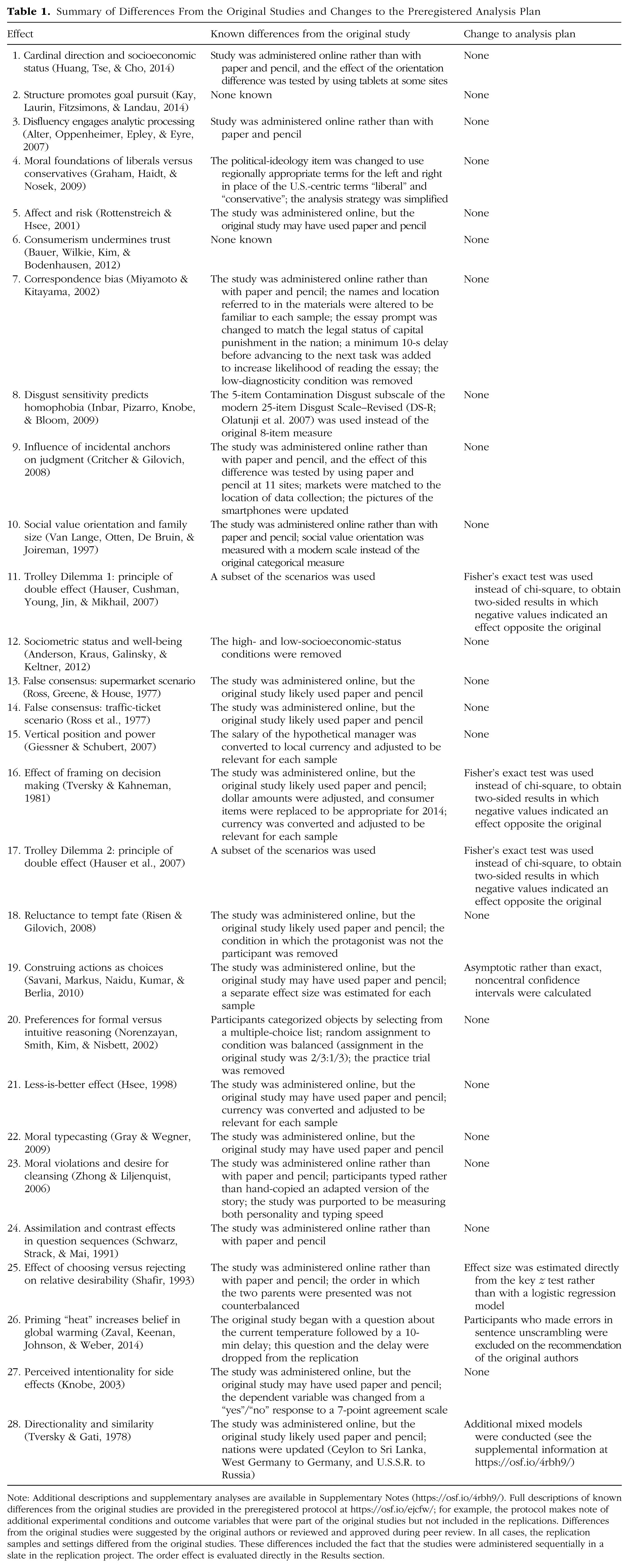
Note: Additional descriptions and supplementary analyses are available in Supplementary Notes (https://osf.io/4rbh9/). Full descriptions of known differences from the original studies are provided in the preregistered protocol at https://osf.io/ejcfw/; for example, the protocol makes note of additional experimental conditions and outcome variables that were part of the original studies but not included in the replications. Differences from the original studies were suggested by the original authors or reviewed and approved during peer review. In all cases, the replication samples and settings differed from the original studies. These differences included the fact that the studies were administered sequentially in a slate in the replication project. The order effect is evaluated directly in the Results section.
Measures
We report how we determined our sample size, all data exclusions, all manipulations, and all measures in the study.
Ethical approval
This research was conducted in accordance with the Declaration of Helsinki and followed local requirements for the institutional review board’s approval at each of the data-collection sites.
Method
Participants
An open invitation to participate as a data-collection site in Many Labs 2 was issued in early 2014. To be eligible for inclusion, labs had to agree to administer their assigned study procedure to at least 80 participants and to collect data from as many as was feasible. Labs decided to stop data collection on the basis of their access to participants and time constraints. None had opportunity to observe the outcomes prior to the conclusion of data collection. All contributors who met the design and data-collection requirements received authorship on this final report. Upon completion of data collection, there were 125 total samples (64 for Slate 1 and 61 for Slate 2; 15 sites collected data for both slates), and the cumulative sample size was 15,305 (mean n = 122.44, median = 99, SD = 92.71, range = 16–841).
For 79 samples, data were collected in person (typically in the lab, though tasks were completed on the Internet), and for 46 samples, data collections was entirely Web based. Thirty-nine of the samples were from the United States, and the 86 others were from Australia (n = 2); Austria (n = 2); Belgium (n = 2); Brazil (n = 1); Canada (n = 4); Chile (n = 3); China (n = 5); Colombia (n = 1); Costa Rica (n = 2); the Czech Republic (n = 3); France (n = 2); Germany (n = 4); Hong Kong, China (n = 3); Hungary (n = 1); India (n = 5); Italy (n = 1); Japan (n = 1); Malaysia (n = 1); Mexico (n = 1); The Netherlands (n = 9); New Zealand (n = 2); Nigeria (n = 1); Poland (n = 6); Portugal (n = 1); Serbia (n = 3); South Africa (n = 3); Spain (n = 2); Sweden (n = 1); Switzerland (n = 1); Taiwan (n = 1); Tanzania (n = 2); Turkey (n = 3); the United Arab Emirates (n = 2); the United Kingdom (n = 4); and Uruguay (n = 1). Details about each site of data collection are available at https://osf.io/uv4qx/.
Of the participants who responded to demographics questions in Slate 1, 34.5% were men, 64.4% were women, 0.3% selected “other,” and 0.8% selected “prefer not to answer.” The average age for Slate 1 participants (after excluding responses greater than “100”) was 22.37 (SD = 7.09). Of the participants in Slate 2, 35.9% were men, 62.9% were women, 0.4% selected “other,” and 0.8% selected “prefer not to answer.” The average age for Slate 2 participants (after excluding responses greater than “100”) was 23.34 (SD = 8.28). Variation in demographic characteristics across the samples is documented at https://osf.io/g3bza/.
Procedure
The tasks were administered over the Internet for purposes of standardization across locations. At some locations, participants completed the survey in a lab or room on computers or tablets, whereas in other locations, participants completed the survey entirely online at their own convenience. Surveys were created in Qualtrics software (qualtrics.com), and a unique link to run the studies was sent to each data-collection team so that we could track the origin of data. Each site was assigned an identifier. These identifiers can be found under the “source” variable in the public data set (available at https://osf.io/8cd4r/).
Data were deposited to a central database and analyzed together. Each team created a video simulation of study administration to illustrate the features of the data-collection setting. Labs that used a language other than English completed a translation of the study materials and then a back-translation to check that the original meaning was retained (cf. Brislin, 1970). Labs decided themselves the language that was appropriate for their sample and adapted materials so that the content would be appropriate for their sample (e.g., some labs edited monetary units).
Labs were assigned to slates so as to maximize the national diversity for both slates. If there was only one lab in a given country, it was randomly assigned to a slate using a tool available at random.org. If there was more than one lab for a country, the labs were also randomly assigned to slates using a tool available at random.org, but with the constraint that the labs were evenly distributed across slates as closely as possible (e.g., two labs in each slate if there were four labs in that country). Near the beginning of data collection, we recruited some additional Asian sites specifically for Slate 1 to increase its sample diversity. The slates were administered by a single experiment script that began with informed consent, next presented the appropriate tasks in an order that was fully randomized across participants, then presented the individual difference measures in randomized order, and closed with demographics measures and debriefing (see Table A2 in the appendix for a list of the demographic, data-quality, and individual difference measures included, with citation counts).
Demographics
Demographic information was collected so that we could characterize each sample and explore possible moderation. Participants were free to decline to answer any question.
Age
Participants noted their age in years in an open-response box.
Sex
Participants selected “male,” “female,” “other,” or “prefer not to answer” to indicate their biological sex.
Race-ethnicity
Participants indicated their race-ethnicity by selecting from a drop-down menu populated with options determined by the lead researcher for each site. Participants could also select “other” or write an open response. Note that response items were not standardized, as different countries have very different conceptualizations of race and ethnicity.
Cultural origins
Three items assessed cultural origins. Each used a drop-down menu populated by a list of countries or territories and an “other” option with an open-response box. The three items were as follows: (a) “In which country/region were you born?”; (b) “In which country/region was your primary caregiver (e.g., parent, grandparent) born?”; and (c) “If you had a second primary caregiver, in which country/region was he or she born?”
Hometown
All participants were asked to indicate their hometown (“What is the name of your home town/city?”) in an open-response box. This item was included for possible future examination as a potential moderator of Huang, Tse, and Cho’s (2014) effect.
Location of wealth in hometown
Another item asked, “Where do wealthier people live in your home town/city?” The response options were “north,” “south,” and “neither.” This item was included as a potential moderator of Huang et al.’s (2014) effect and appeared in Slate 1 only.
Political ideology
Participants rated their political ideology on a scale with response options of “strongly left-wing,” “moderately left-wing,” “slightly left-wing,” “moderate,” “slightly right-wing,” “moderately right-wing,” and “strongly right-wing.” Instructions were adapted for each country to ensure this measure’s relevance to the local context. For example, the U.S. instructions read: “Please rate your political ideology on the following scale. In the United States, ‘liberal’ is usually used to refer to left-wing and ‘conservative’ is usually used to refer to right-wing.”
Education
Participants reported their educational attainment in response to a single item, “What is the highest educational level that you have attained?” The response scale was as follows: 1 = no formal education, 2 = completed primary/elementary school, 3 = completed secondary school/high school, 4 = some university/college, 5 = completed university/college degree, 6 = completed advanced degree.
Socioeconomic status
Socioeconomic status (SES) was measured with the ladder technique (Adler et al., 1994). Participants used a ladder with 10 steps to indicate their standing in the community with which they most identified relative to other people in that community. On the ladder, 1 indicated people having the lowest standing in the community, and 10 referred to people having the highest standing. Previous research demonstrated that this item has good convergent validity with objective criteria of individual social status and also good construct validity with regard to several psychological and physiological health indicators (e.g., Adler, Epel, Castellazzo, & Ickovics, 2000; S. Cohen et al., 2008). This ladder was also used as one of the items for Anderson, Kraus, Galinsky, and Keltner’s (2012, Study 3) effect in Slate 1. Participants in that slate answered the ladder item as part of the materials for that effect and did not receive the item a second time.
Data quality
Recent research on careless responding or insufficient effort in responding has suggested that there is a need to refine implementation of established scales embedded in data collection to check for aberrant response patterns (Huang et al., 2014; Meade & Craig, 2012). As a check on data quality, we included two items at the end of the study, just prior to the demographic items. The first item asked participants, “In your honest opinion, should we use your data in our analyses in this study?” and had “yes” and “no” as response options (Meade & Craig, 2012). The second item was an instructional manipulation check (Oppenheimer, Meyvis, & Davidenko, 2009), in which an ostensibly simple demographic question (“Where are you completing this study?”) was preceded by a long block of text that contained, in part, alternative instructions for participants to follow to demonstrate that they were paying attention (“Instead, simply check all four boxes and then press ‘continue’ to proceed to the next screen”).
Individual difference measures
The following individual difference measures were included to allow future tests of effect-size moderation.
Cognitive reflection
The cognitive-reflection task (CRT; Frederick, 2005) assesses individuals’ ability to suppress an intuitive (wrong) response in favor of a deliberative (correct) answer. The items on the original CRT are widely known, and the measure is vulnerable to practice effects (Chandler, Mueller, & Paolacci, 2014). Therefore, we used an updated version that is logically equivalent and correlates highly with the items on the original CRT (Finucane & Gullion, 2010). The three items are (a) “If it takes 2 nurses 2 minutes to measure the blood pressure of 2 patients, how long would it take 200 nurses to measure the blood pressure of 200 patients?”; (b) “Soup and salad cost $5.50 in total. The soup costs a dollar more than the salad. How much does the salad cost?”; and (c) “Sally is making tea. Every hour, the concentration of the tea doubles. If it takes 6 hours for the tea to be ready, how long would it take for the tea to reach half of the final concentration?” Also, we constrained the total time available to answer the three questions to 75 s. This likely lowered overall performance on average, as it was somewhat less time than some participants took in pretesting.
Subjective well-being
Subjective well-being was measured with a single item: “All things considered, how satisfied are you with your life as a whole these days?” The response scale ranged from 1, dissatisfied, to 10, satisfied. Similar items have been included in numerous large-scale social surveys (cf. Veenhoven, 2009) and have shown satisfactory reliability (e.g., Lucas & Donnellan, 2012) and validity (Cheung & Lucas, 2014; Oswald & Wu, 2010; Sandvik, Diener, & Seidlitz, 1993).
Global self-esteem
Global self-esteem was measured using the Single-Item Self-Esteem Scale (Robins, Hendin, & Trzesniewski, 2001), which was designed as an alternative to the Rosenberg (1965) Self-Esteem Scale. The SISE consists of a single item: “I have high self-esteem.” Participants respond on a 5-point Likert scale, ranging from 1, not very true of me, to 5, very true of me. Robins et al. reported that the SISE has strong convergent validity with the Rosenberg Self-Esteem Scale among adults (rs ranging from .70 to .80) and that the SISE and Rosenberg Self-Esteem Scale have similar predictive validity.
Big Five personality
The five basic traits of human personality (Goldberg, 1981)—conscientiousness, agreeableness, neuroticism (emotional stability), openness (intellect), and extraversion—were measured with the Ten-Item Personality Inventory (Gosling, Rentfrow, & Swann, 2003). Each trait was assessed with two items answered on response scales from 1, disagree strongly, to 7, agree strongly. The five scales have satisfactory retest reliability (cf. Gnambs, 2014) and substantial convergent validity with longer Big Five instruments (e.g., Ehrhart et al., 2009; Gosling et al., 2003; Rojas & Widiger, 2014).
Mood
There exist many assessments of mood. We selected the single item from G. L. Cohen et al. (2007): “How would you describe your mood right now?” The response options are as follows: 1 = extremely bad, 2 = bad, 3 = neutral, 4 = good, 5 = extremely good.
Disgust sensitivity
To measure disgust sensitivity, we used the Contamination Disgust subscale of the Disgust Scale–Revised (DS-R; Olatunji et al., 2007), a 25-item revision of the original Disgust Sensitivity Scale (Haidt, McCauley, & Rozin, 1994). The subscales of the DS-R were determined by factor analysis. The Contamination Disgust subscale includes 5 items related to concerns about bodily contamination. Because of length considerations, this subscale was included only in Slate 1, for Inbar, Pizarro, Knobe, and Bloom’s (2009, Study 1) effect. No part of the DS-R appeared in Slate 2.
The 28 Effects
Before presenting the main results for heterogeneity across samples and settings, we discuss each of the 28 selected effects. For each effect, we summarize the main idea of the original research, provide the sample size, and present the inferential test and effect size that were the target for replication. Then, we summarize the aggregate result of the replication. For these aggregate tests, we pooled the data of all available samples, ignoring sample origin. An aggregate result was labeled consistent with the original finding if the effect was statistically significant and in the same direction as in the original study. The vast majority of the original studies were conducted in a Western, educated, industrialized, rich, democratic (i.e., WEIRD) society (Henrich, Heine, & Norenzayan, 2010). For the four original studies that focused on cultural differences, we present the replication results such that positive effect sizes correspond to the direction of the effect that had been observed in the original WEIRD sample. Our main replication result is the aggregate effect size regardless of cultural context. Whether effects varied by setting (or cultural context more generally) was examined in the heterogeneity analyses reported in the Results section. Heterogeneity was assessed using the Q, tau, and I2 measures (Borenstein, Hedges, Higgins, & Rothstein, 2009). If there was opportunity to test the original cultural difference with similar samples, we did so, and these additional results are reported in this section. If the original authors anticipated moderating influences that could affect comparison of the original and replication effect sizes, then we also report those analyses.
Readers interested in the global results of this replication project may skip this long section detailing each individual replication and proceed to the section presenting the systematic meta-analyses testing variation by sample and setting.
Slate 1
1. Cardinal direction and socioeconomic status (Huang et al., 2014, Study 1a)
People in the United States and Hong Kong have different demographic knowledge that may shape their metaphoric association between valence and cardinal direction (north vs. south). One hundred eighty participants from the United States and Hong Kong participated in Huang et al.’s (2014) Study 1a. They were presented with a blank map of a fictional city and were randomly assigned to indicate on the map where either a high-SES or a low-SES person might live. There was an interaction between SES (high vs. low) and population (United States vs. Hong Kong), F(1, 176) = 20.39, MSE = 5.63, p < .001, η p 2 = .10, d = 0.68, 95% confidence interval (CI) = [0.38, 0.98]. U.S. participants expected the high-SES person to live further north (M = 0.98, SD = 1.85) than the low-SES person (M = −0.69, SD = 2.19), t(78) = 3.69, p < .001, d = 0.83, 95% CI = [0.37, 1.28]. Conversely, Hong Kong participants expected the low-SES person to live further north (M = 0.63, SD = 2.75) than the high-SES person (M = −0.92, SD = 2.47), t(98) = −2.95, p = .004, d = −0.59, 95% CI = [−0.99, −0.19]. The authors explained that wealth in Hong Kong is concentrated in the south of the city, and wealth in cities in the United States is more commonly concentrated in the north of the city. As a consequence, members of these cultures differ in their assumptions about the concentration of wealth in fictional cities.
Replication
The coordinates of participants’ clicks on the fictional map were recorded (x, y) from the top left of the image and then recentered in the analysis such that clicks in the north half of the map were positive and clicks in the southern half of the map were negative. Across all samples (N = 6,591), participants in the high-SES condition (M = 11.70, SD = 84.31) selected a further north location than did participants in the low-SES condition (M = −22.70, SD = 88.78), t(6554.05) = 16.12, p = 2.15e−57, d = 0.40, 95% CI = [0.35, 0.45].
As suggested by the original authors, the focal test for replicating the effect they found for Western participants was completed by selecting only those participants, across all samples, who indicated that wealth tended to be in the north in their hometown. These participants expected the high-SES person to live further north (M = 43.22, SD = 84.43) than the low-SES person (M = −40.63, SD = 84.99), t(1692) = 20.36, p = 1.24e−82, d = 0.99, 95% CI = [0.89, 1.09]. This result is consistent with the hypothesis that people reporting that wealthier people tend to live in the north in their hometown also guess that wealthier people will tend to live in the north in a fictional city, and the effect was substantially larger than that in the sample as a whole.
Follow-up analyses
The original study compared Hong Kong and U.S. participants. In the replication, Hong Kong participants expected the high-SES person to live further south (M = −37.44, SD = 84.29) than the low-SES person (M = 12.43, SD = 95.03), t(140) = −3.30, p = .001, d = −0.55, 95% CI = [−0.89, −0.22]. U.S. participants expected the high-SES person to live further north (M = 41.55, SD = 80.73) than the low-SES person (M = −42.63, SD = 82.41), t(2199) = 24.20, p = 6.53e−115, d = 1.03, 95% CI = [0.94, 1.12]. This result is consistent with the original finding that cultural differences in perceived location of wealth in a fictional city correlated with location of wealth in participants’ hometown.
Most participants completed the items for this study on a vertically oriented monitor display as opposed to a paper survey on a desk, as in the original study. The original authors suggested a priori that this difference might be important because associations between “up” and “good” or between “down” and “bad” might interfere with any associations with “north” and “south.” At 10 data-collection sites (n = 582), we assigned some participants to complete Slate 1 on Microsoft Surface tablets resting horizontally on a table. Among the participants using the horizontal tablets, those who said that wealth tended to be in the north in their hometown (n = 156) expected the high-SES person to live further north (M = 38.66, SD = 80.43) than the low-SES person (M = −43.92, SD = 80.32), t(154) = 6.38, p = 1.95e−09, d = 1.03, 95% CI = [0.69, 1.36]. By comparison, within this horizontal-tablet group, participants who said that wealth tended to be in the south in their hometown (n = 87) expected the high-SES person to live further south (M = −33.58, SD = 72.89) than the low-SES person (M = −4.11, SD = 88.33), t(85) = −1.63, p = .11, d = −0.36, 95% CI = [−0.79, 0.08]. The effect sizes for just these subsamples were very similar to the effect sizes for the whole sample, which suggests that the orientation of the display did not moderate this effect.
2. Structure promotes goal pursuit (Kay, Laurin, Fitzsimons, & Landau, 2014, Study 2)
In Study 2 of Kay et al. (2014), 67 participants generated what they felt was their most important goal. They then read one of two scenarios in which a natural event (leaves growing on trees) was described as being a structured or random event. For example, in the structured condition, a sentence read, “The way trees produce leaves is one of the many examples of the orderly patterns created by nature …, ” but in the random condition, the corresponding sentence read, “The way trees produce leaves is one of the many examples of the natural randomness that surrounds us. . . .” Next, participants answered three questions about their most important goal, on a scale from 1, not very, to 7, extremely. The first item measured the subjective value of the goal, and the other two items measured willingness to pursue that goal. Participants exposed to a structured event (M = 5.26, SD = 0.88) were more willing to pursue their goal compared with those exposed to a random event (M = 4.72, SD = 1.32), t(65) = 2.00, p = .05, d = 0.49, 95% CI = [0.001, 0.973]. In the overall replication sample (N = 6,506), participants exposed to a structured event (M = 5.48, SD = 1.45) were not significantly more willing to pursue their goal compared with those exposed to a random event (M = 5.51, SD = 1.39), t(6498.63) = −0.94, p = .35, d = −0.02, 95% CI = [−0.07, 0.03]. This result does not support the hypothesis that willingness to pursue goals is higher after exposure to structured as opposed to random events.
3. Disfluency engages analytic processing (Alter, Oppenheimer, Epley, & Eyre, 2007, Study 4)
In Study 4, Alter et al. (2007) investigated whether a deliberate, analytic processing style can be activated by incidental disfluency cues that suggest task difficulty. Forty-one participants attempted to solve syllogisms presented in either a hard-to-read or an easy-to-read font. The hard-to-read font served as an incidental induction of disfluency. Participants in the hard-to-read-font condition answered more moderately difficult syllogisms correctly (64%) than did participants in the easy-to-read-font condition (42%), t(39) = 2.01, p = .051, d = 0.63, 95% CI = [−0.004, 1.25].
Replication
The original study focused on the two moderately difficult syllogisms among the six administered. Our analysis strategy was sensitive to potential differences across samples in ability to solve the syllogisms. We first determined which ones were moderately difficult for participants by excluding within each sample any syllogisms that were answered correctly by fewer than 25% of participants or more than 75% of participants in the two conditions combined. The remaining syllogisms were used to calculate mean syllogism performance for each participant.
As in Alter et al.’s (2007) experiment, the easy-to-read font was 12-point black Myriad Web font, and the hard-to-read font was 10-point 10% gray italicized Myriad Web font. For a direct comparison with the original effect size, the original authors suggested that only English in-lab samples be used for two reasons: First, we could not adequately control for online participants “zooming in” on the page or otherwise making the font more readable, and second, we anticipated having to substitute the font in some translated versions because the original font (Myriad Web) might not support all languages. 2 In this subsample (N = 2,580), the number of syllogisms answered correctly by participants in the hard-to-read-font condition (M = 1.10, SD = 0.88) was similar to the number answered correctly by participants in the easy-to-read-font condition (M = 1.13, SD = 0.91), t(2578) = −0.79, p = .43, d = −0.03, 95% CI = [−0.08, 0.01]. In a secondary analysis that mirrored the original, we used performance on the same two syllogisms Alter et al. (2007) focused on. Again, the number of syllogisms answered correctly by participants in the hard-to-read-font condition (M = 0.80, SD = 0.79) was similar to the number answered correctly by participants in the easy-to-read-font condition (M = 0.84, SD = 0.81), t(2578) = −1.19, p = .23, d = −0.05, 95% CI = [−0.12, 0.03]). 3 These results do not support the hypothesis that syllogism performance is higher when the font is harder to read; the difference between conditions was slightly in the opposite direction and not distinguishable from zero (d = −0.03, 95% CI = [−0.08, 0.01], vs. original d = 0.64).
Follow-up analyses
In the aggregate replication sample (N = 6,935), the number of syllogisms answered correctly was similar in the hard-to-read-font condition (M = 1.03, SD = 0.86) and the easy-to-read-font condition (M = 1.06, SD = 0.87), t(6933) = −1.37, p = .17, d = −0.03, 95% CI = [−0.08, 0.01]. Finally, in the whole sample, an analysis using the same two syllogisms that Alter et al. (2007) did showed that participants in the hard-to-read-font condition answered about as many syllogisms correctly (M = 0.75, SD = 0.76) as participants in the easy-to-read-font condition (M = 0.79, SD = 0.77), t(6933) = −2.07, p = .039, d = −0.05, 95% CI = [−0.097, −0.003]. These follow-up analyses do not qualify the conclusion from the focal tests.
4. Moral foundations of liberals versus conservatives (Graham, Haidt, & Nosek, 2009, Study 1)
People on the political left (liberal) and political right (conservative) have distinct policy preferences and may also have different moral intuitions and principles. In Graham et al.’s (2009) Study 1, 1,548 participants across the ideological spectrum rated whether different concepts, such as “purity” and “fairness,” were relevant for deciding whether something was right or wrong. Items that emphasized concerns of harm or fairness (individualizing foundations) were deemed more relevant for moral judgment by the political left than by the political right (r = −.21, d = −0.43, 95% CI = [−0.55, −0.32]), whereas items that emphasized concerns for the in-group, authority, or purity (binding foundations) were deemed more relevant for moral judgment by the political right than by the political left (r = .25, d = 0.52, 95% CI = [0.40, 0.63]). 4 Participants rated the relevance to moral judgment of 15 items (3 for each foundation) in a randomized order on a 6-point scale from not at all relevant to extremely relevant.
Replication
The primary target of replication was the relationship between political ideology and the binding foundations. In the aggregate sample (N = 6,966), items that emphasized concerns for the in-group, authority, or purity were deemed more relevant for moral judgment by the political right than by the political left (r = .14, p = 6.05e−34, d = 0.29, 95% CI = [0.25, 0.34], q = 0.15, 95% CI = [0.12, 0.17]). This result is consistent with the hypothesis that binding foundations are perceived as more morally relevant by members of the political right than by members of the political left. The overall effect size was smaller than the original (d = 0.29, 95% CI = [0.25, 0.34], vs. original d = 0.52).
Follow-up analyses
The relationship between political ideology and the individualizing foundations was a secondary replication target. In the aggregate sample (N = 6,970), items that emphasized concerns of harm or fairness were deemed more relevant for moral judgment by the political left than by the political right (r = −.13, p = 2.54e−29, d = −0.27, 95% CI = [−0.32, −0.22], q = −0.13, 95% CI = [−0.16, −0.11]). This result is consistent with the hypothesis that individualizing foundations are perceived as more morally relevant by members of the political left than by members of the political right. The overall effect size was smaller than the original result (d = −0.27, 95% CI = [−0.32, −0.22], vs. original d = −0.43).
5. Affect and risk (Rottenstreich & Hsee, 2001, Study 1)
In this experiment, 40 participants chose whether they would prefer an affectively attractive option (a kiss from a favorite movie star) or a financially attractive option ($50). In one condition, participants made the choice imagining a low probability (1%) of getting the outcome. In the other condition, participants imagined that the outcome was certain, and they just needed to choose between the options. When the outcome was unlikely, 70% of participants preferred the affectively attractive option; when the outcome was certain, 35% preferred the affectively attractive option. The difference between conditions was significant, χ2(1, N = 40) = 4.91, p = .0267, d = 0.74, 95% CI = [< 0.001, 1.74]. This result supported the hypothesis that positive affect has greater influence on judgments about uncertain outcomes than on judgments about definite outcomes.
In the aggregate replication sample (N = 7,218), when the outcome was unlikely, 47% of participants preferred the affectively attractive choice, and when the outcome was certain, 51% preferred the affectively attractive choice. The difference was significant, p = .002, odds ratio (OR) = 0.87, d = −0.08, 95% CI = [−0.13, −0.03], but in the direction opposite the prediction of the hypothesis (i.e., that affectively attractive choices are more preferred when they are uncertain rather than definite). The overall effect was much smaller than in the original study and in the opposite direction (d = −0.08, 95% CI = [−0.13, −0.03], vs. original d = 0.74).
6. Consumerism undermines trust (Bauer, Wilkie, Kim, & Bodenhausen, 2012, Study 4)
Bauer et al. (2012) examined whether being in a consumer mind-set would reduce trust in other people. In their Study 4, 77 participants read about a hypothetical water-conservation dilemma in which they were involved. They were randomly assigned to either a condition that referred to them and other people in the scenario as “consumers” or a condition that referred to them and other people in the scenario as “individuals” (control condition). Participants in the consumer condition reported less trust that other people would conserve water (M = 4.08, SD = 1.56; scale from 1, not at all, to 7, very much) compared with participants in the control condition (M = 5.33, SD = 1.30), t(76) = 3.86, p = .001, d = 0.87, 95% CI = [0.41, 1.34].
Replication
In the aggregate replication sample (N = 6,608), participants in the consumer condition reported slightly less trust that other people would conserve water (M = 3.92, SD = 1.44) compared with participants in the control condition (M = 4.10, SD = 1.45), t(6606) = 4.93, p = 8.62e−7, d = 0.12, 95% CI = [0.07, 0.17]. This result is consistent with the hypothesis that people have lower trust in others when they think of those others as consumers rather than as individuals. The overall effect size was much smaller than in the original experiment (d = 0.12, 95% CI = [0.07, 0.17], vs. original d = 0.87).
Follow-up analyses
The original experiment and the replication examined the effect of the priming manipulation on four additional dependent variables. Compared with the original study, the replication showed weaker effects in the same direction for (a) participants’ feelings of responsibility for the crisis (original d = 0.47; replication d = 0.10, 95% CI = [0.05, 0.15]), (b) participants’ feelings of obligation to cut water usage (original d = 0.29; replication d = 0.08, 95% CI = [0.03, 0.13]), (c) participants’ perception of other people as partners (original d = 0.53; replication d = 0.12, 95% CI = [0.07, 0.16]), and (d) participants’ judgments about how much less water other people should use (original d = 0.25; replication d = 0.01, 95% CI = [−0.04, 0.06]).
7. Correspondence bias (Miyamoto & Kitayama, 2002, Study 1)
Miyamoto and Kitayama (2002) examined whether Americans would be more likely than Japanese to show a bias toward ascribing to an actor an attitude corresponding to the actor’s behavior, a phenomenon referred to as correspondence bias (Jones & Harris, 1967). In their Study 1, 49 Japanese and 58 American undergraduates learned that they would read a university student’s essay about the death penalty and infer the student’s true attitude toward the issue. The essay was either in favor of or against the death penalty, and it was designed to be diagnostic or not very diagnostic of a strong attitude. After reading the essay, participants learned that the student had been assigned which position to argue. Then, participants estimated the essay writer’s actual attitude toward capital punishment and the extent to which they thought the student’s behavior was constrained by the assignment.
Controlling for perceived constraint, analyses compared perceived attitudes of the writer who wrote in favor of capital punishment and the writer who wrote against it (rating scale from 1, against capital punishment, to 15, supports capital punishment). American participants perceived a large difference between the actual attitude of the essay writer who had been assigned to write a pro-capital-punishment essay (M = 10.82, SD = 3.47) and the writer who had been assigned to write an anti-capital-punishment essay (M = 3.30, SD = 2.62), t(27) = 6.66, p < .001, d = 2.47, 95% CI = [1.46, 3.49]. Japanese participants perceived less of a difference in actual attitudes (M = 9.27, SD = 2.88, and M = 7.02, SD = 3.06, respectively), t(23) = 1.84, p = .069, d = 0.74, 95% CI = [–0.12, 1.59].
Replication
In the aggregate replication sample (N = 7,197), controlling for perceived constraint, participants perceived a difference in actual attitudes between the essay writer who had been assigned to write a pro-capital-punishment essay (M = 10.98, SD = 3.69) and the essay writer who had been assigned to write an anti-capital-punishment essay (M = 4.45, SD = 3.51), F(2, 7194) = 3,042.00, p < 2.2e−16, d = 1.82, 95% CI = [1.76, 1.87]. This finding is consistent with the correspondence-bias hypothesis: Participants inferred the essay writer’s attitude, in part, on the basis of the writer’s observed behavior. Whether the magnitude of this effect varies cross-culturally was examined in tests discussed in the Results section.
Follow-up analyses
Results for the primary replication analysis showed that participants estimated the writer’s true attitude toward capital punishment to be similar to the position that the writer was assigned to defend. Participants also expected that the writers would express attitudes consistent with the position to which they were assigned if given the opportunity to talk freely about capital punishment (pro–capital punishment: M = 10.17, SD = 3.84; anti–capital punishment: M = 4.96, SD = 3.61), t(7187) = 59.44, p = 2.2e−16, d = 1.40, 95% CI = [1.35, 1.45].
Two possible moderators were included in the design: perceived attitude of the average student in the writer’s country (tailored to be the same as the participant’s country) and perceived persuasiveness of the essay. In the aggregate replication sample (N = 7,211), controlling for perceived constraint, we did not observe an interaction between condition and perceived attitude of the average student in the writer’s country on estimations of the writer’s true attitude toward capital punishment, t(7178) = 0.55, p = .58, d = 0.013, 95% CI = [−0.03, 0.06]. We did, however, observe an interaction between condition and perceived persuasiveness of the essay on estimations of the writer’s true attitude toward capital punishment, t(7170) = 16.25, p = 2.3e−58, d = 0.38, 95% CI = [0.34, 0.43]. The effect of condition on estimations of the writer’s true attitude toward capital punishment was stronger for higher levels of perceived persuasiveness of the essay.
8. Disgust sensitivity predicts homophobia (Inbar et al., 2009, Study 1)
Behaviors that are deemed morally wrong may be judged as more intentional than behaviors without moral implications (Knobe, 2006). Thus, people who judge the portrayal of gay sexual activity in the media as intentional may view homosexuality as morally reprehensible. In Inbar et al.’s (2009) Study 1, 44 participants read a vignette about a director’s action and judged him as more intentional (scale from 1, not at all, to 7, definitely) when he was described as encouraging gay kissing (M = 4.36, SD = 1.51) than when he was describing more generally as encouraging kissing (M = 2.91, SD = 2.01), β = 0.41, t(39) = 3.39, p = .002, r = .48. Disgust sensitivity was positively related to judgments of intentionality in the gay-kissing condition, β = 0.79, t(19) = 4.49, p = .0003, r = .72, and not the kissing condition, β = −0.20, t(19) = −0.88, p = .38, r = .20. The correlation was stronger in the gay-kissing condition than in the kissing condition, z = 2.11, p = .03, q = 0.70, 95% CI = [0.05, 1.36]. The authors concluded that individuals who are more prone to disgust are more likely to interpret encouragement of gay kissing as intentional, which indicates that they intuitively disapprove of homosexuality.
Replication
The relationship between disgust sensitivity and intentionality ratings was the target of our direct replication. In the aggregate replication sample (N = 7,117), participants did not judge the director’s action as more intentional when he encouraged gay kissing (M = 3.48, SD = 1.87) than when he encouraged kissing (M = 3.51, SD = 1.84), t(7115) = −0.74, p = .457, d = −0.02, 95% CI = [−0.06, 0.03]. Greater disgust sensitivity was related to judgments of greater intentionality in both the gay-kissing condition, r = .12, p = 1.2e−13, and the kissing condition, r = .07, p = 2.48e−5. The correlation in the gay-kissing condition was similar to the correlation in the kissing condition, z = 2.62, p = .02, q = 0.05, 95% CI = [0.01, 0.10]. These data are inconsistent with the original finding that disgust sensitivity and perceived intentionality are more strongly related when people consider gay kissing than when they consider kissing in general, and the effect size was much smaller than the original effect size (q = 0.05, 95% CI = [0.01, 0.10], vs. original q = 0.70). Disgust sensitivity was very weakly related to perceived intentionality, and there was no mean difference in perceived intentionality between the gay-kissing and kissing conditions.
Follow-up analyses
The original study included two other outcome measures based on responses to yes/no questions. These were examined as secondary replications following the same analysis strategy as for intentionality. First, disgust sensitivity was only slightly more related to responses to “Is there anything wrong with homosexual men French kissing in public?” (r = −.20, p < 2.2e−16) than to responses to “Is there anything wrong with couples French kissing in public?” (r = −.16, p < 2.2e−16; z = −1.66, p = .096, q = −0.04, 95% CI = [−0.09, 0.01]). Second, disgust sensitivity was only slightly more related to answers to “Was it wrong of the director to make a video that he knew would encourage homosexual men to French kiss in public?” (r = .27, p < 2.2e−16) than to “Was it wrong of the director to make a video that he knew would encourage couples to French kiss in public?” (r = .22, p < 2.2e−16; z = 2.28, p = .02, q = 0.05, 95% CI = [0.01, 0.10]).
9. Influence of incidental anchors on judgment (Critcher & Gilovich, 2008, Study 2)
In Critcher and Gilovich’s (2008) Study 2, 207 participants predicted the relative popularity of a new cell phone in the U.S. and European marketplaces. In one condition, the smartphone was called the P97; in the other condition, the smartphone was called the P17. Participants in the P97 condition estimated that a greater percentage of the new phone’s sales would be in the United States (M = 58.1%, SD = 19.6%) compared with participants in the P17 condition (M = 51.9%, SD = 21.7%), t(197.5) = 2.12, p = .03, d = 0.30, 95% CI = [0.02, 0.58]. This result supported the hypothesis that judgment can be influenced by incidental anchors in the environment. The mere presence of a high or low number in the name of the cell phone influenced estimates of sales of the phone.
Replication
In the aggregate replication sample (N = 6,826), participants’ estimates of the percentage of sales the new phone would garner in their region as opposed to a foreign market were approximately the same in the P97 condition (M = 49.87%, SD = 21.86%) as in the P17 condition (M = 48.98%, SD = 22.14%), t(6824) = 1.68, p = .09, d = 0.04, 95% CI = [−0.01, 0.09]. This result does not support the hypothesis that sales estimates are influenced by incidental anchors. The effect size was in the same direction as the original effect size, but much smaller (d = 0.04, 95% CI = [−0.01, 0.09], vs. original d = 0.30) and indistinguishable from zero.
Follow-up analyses
The original authors administered this experiment with paper and pencil, rather than on a computer, to avoid the possibility that the numeric keys on the keyboard might serve as primes. We administered this task with paper and pencil at 11 sites. At these sites (N = 1,112), participants in the P97 condition estimated that the new phone’s percentage of sales in their region would be slightly smaller (M = 53.02%, SD = 20.15%) compared with participants in the P17 condition (M = 53.28%, SD = 20.17%), t(1110) = −0.22, p = .83, d = −0.01, 95% CI = [−0.13, 0.10]. This difference was in the direction opposite the direction of the original finding, but not reliably different from zero.
10. Social value orientation and family size (Van Lange, Otten, De Bruin, & Joireman, 1997, Study 3)
Van Lange et al. (1997) proposed that social value orientations (SVOs) are rooted in social interaction experiences, and that the number of one’s siblings is one variable that influences such experiences. In one of four studies (Study 3), they examined the association between SVO and family size, thereby providing a test of two competing hypotheses. One hypothesis states that in larger families, resources have to be shared more frequently, and this facilitates cooperation and the development of a prosocial orientation. Another hypothesis, rooted in group-size effects, states that greater family size may undermine trust and expected cooperation from other people, and may therefore inhibit the development of prosocial orientation. In Study 3, 631 participants reported how many siblings they had and completed an SVO measure called the Triple-Dominance Measure, which identified them as prosocial people, individualists, or competitors. An analysis of variance (ANOVA) revealed a significant difference in SVO across these groups, F(2, 535) = 4.82, p = .01. Prosocial people had more siblings (M = 2.03, SD = 1.56) than individualists (M = 1.63, SD = 1.00) and competitors (M = 1.71, SD = 1.35), ds = 0.287, 95% CI = [0.095, 0.478], and 0.210, 95% CI = [−0.045, 0.465], respectively. Planned comparisons of the number of siblings revealed a significant contrast between prosocial people, on the one hand, and individualists and competitors, on the other, F(1, 535) = 9.14, p = .003, d = 0.19, 95% CI = [< 0.01, 0.47].
The original demonstration used a measure of SVO with three categorical values. In discussion with the original first author, an alternative measure, the SVO slider (Murphy, Ackermann, & Handgraaf, 2011), was identified as a useful replacement to yield a continuous distribution of scores. Thus, the replication focused only on the observed direct positive correlation between prosocial orientation and number of siblings. In the aggregate replication sample (N = 6,234), number of siblings was not related to prosocial orientation (r = −.02, 95% CI = [−0.04, 0.01], p = .18). This result does not support the hypothesis that having more siblings is positively related with prosocial orientation. Direct comparison of effect sizes was not possible because of the change in the SVO measure, but the replication effect size was near zero.
11. Trolley Dilemma 1: principle of double effect (Hauser, Cushman, Young, Jin, & Mikhail, 2007, Scenarios 1 and 2)
According to the principle of double effect, an act that harms other people is more morally permissible if the act is a foreseen side effect rather than the means to the greater good. Hauser et al. (2007) compared participants’ reactions to two scenarios to test whether their judgments followed this principle. In the foreseen-side-effect scenario, a person on an out-of-control train changed the train’s trajectory so that the train killed one person instead of five. In the greater-good scenario, a person pushed a fat man in front of a train, killing him, to save five people. Whereas 89% of participants judged the action in the foreseen-side-effect scenario as permissible (95% CI = [87%, 91%]), only 11% of participants in the greater-good scenario judged it as permissible (95% CI = [9%, 13%]). The difference between the percentages was significant, χ2(1, N = 2,646) = 1,615.96, p < .001, w = .78, d = 2.50, 95% CI = [2.22, 2.86]. Thus, the results provided evidence for the principle of double effect.
Replication
In the aggregate replication sample (N = 6,842 after removing participants who responded in less than 4 s), 71% of participants judged the action in the foreseen-side-effect scenario as permissible, but only 17% of participants in the greater-good scenario judged it as permissible. The difference between the percentages was significant, p = 2.2e−16, OR = 11.54, d = 1.35, 95% CI = [1.28, 1.41]. The replication results were consistent with the double-effect hypothesis, and the effect was about half the magnitude of the original (d = 1.35, 95% CI = [1.28, 1.41], vs. original d = 2.50).
Follow-up analyses
Variations of the trolley problem are well known. The original authors suggested that the effect may be weaker for participants who have previously been exposed to this sort of task. We included an additional item assessing participants’ prior knowledge of the task. Among the 3,069 participants reporting that they were not familiar with the task, Cohen’s d was 1.47, 95% CI = [1.38, 1.57]; among the 4,107 who reported being familiar with the task, Cohen’s d was 1.20, 95% CI = [1.12, 1.28]. This suggests moderation by task familiarity, but the effect was very strong regardless of familiarity.
12. Sociometric status and well-being (Anderson et al., 2012, Study 3)
Anderson et al. (2012) examined the relationships among sociometric status (SMS), SES, and subjective well-being. According to the authors, SMS refers to interpersonal wealth, whereas SES refers to fiscal wealth. Study 3 examined whether SMS has stronger ties than SES to well-being. In a 2 × 2 between-participants design, 228 Mechanical Turk participants were presented with descriptions of people who were either relatively high or relatively low on either SES or SMS and then made upward or downward social comparisons (e.g., participants in the high-SMS condition imagined and compared themselves with a low-SMS person). Then, participants wrote about what it would be like to interact with such people, and then reported their subjective well-being. Results showed a significant 2 × 2 interaction, F(1, 224) = 4.73, p = .03. Participants in the high-SMS condition had higher subjective well-being than those in the low-SMS condition, t(115) = 3.05, p = .003, d = 0.57, 95% CI = [0.20, 0.93], but there were no differences between the two SES conditions, t(109) = 0.06, p = .96, d = 0.01.
For replication, we used only the high- and low-SMS conditions and excluded the high- and low-SES conditions because they showed no differences in the original study. In the aggregate replication sample (N = 6,905), participants in the high-SMS condition (M = −0.01, SD = 0.67) had slightly lower subjective well-being than those in the low-SMS condition (M = 0.01, SD = 0.66; scores were standardized and averaged), t(6903) = −1.76, p = .08, d = −0.04, 95% CI = [−0.09, 0.004]. This result did not support the hypothesis that subjective well-being is higher for participants exposed to descriptions of higher SMS. The effect was small in magnitude, much smaller than the original effect, and in the opposite direction (d = −0.04, 95% CI = [−0.09, 0.004], vs. original d = 0.57).
13. False consensus: supermarket scenario (Ross, Greene, & House, 1977, Study 1)
People perceive a false consensus regarding how common their own responses are among other people (Ross et al., 1977). Thus, estimates of the prevalence of a particular belief, opinion, or behavior are biased in the direction of the perceiver’s belief, opinion, or behavior. In Study 1, Ross et al. presented 320 college undergraduates with one of four hypothetical events that culminated in a clear dichotomous choice of action. Participants first estimated what percentage of their peers would choose each option and then indicated their own choice. For each of the four scenarios, participants who chose the first option, compared with those who chose the second, believed that a higher percentage of other people would choose the first option (M = 65.7% vs. 48.5%), F(1, 312) = 49.1, p < .001, d = 0.79, 95% CI = [0.56, 1.02]. A later meta-analysis suggested that this effect is robust and moderate in size across a variety of paradigms (r = .31, Mullen et al., 1985).
This study was replicated in Slate 1 and Slate 2 using different scenarios. In Slate 1, participants were presented with the supermarket vignette, which had shown a significant effect in the original study, F(1, 78) = 17.7, d = 0.99, 95% CI = [0.24, 2.29]. All participants who provided percentage estimates between 0 and 100 and responded to all three items were included in the analysis. In the aggregate replication sample (N = 7,205), participants who chose the first option, compared with those who chose the second, believed that a higher percentage of other people would choose the first option (M = 69.19% vs. 43.35%), t(6420.77) = 49.93, p < 2.2e−16, d = 1.18, 95% CI = [1.13, 1.23]. This result is consistent with the hypothesis that participants’ choices are positively correlated with their perception of the percentage of other people who would make the same choice.
Slate 2
14. False consensus: traffic-ticket scenario (Ross et al., 1977, Study 1)
In Slate 2, participants were presented with the traffic-ticket vignette, which had shown a significant effect in Ross et al.’s (1977) Study 1 (see the previous paragraph for a description of that study), F(1, 78) = 12.8, d = 0.80, 95% CI = [0.22, 1.87]. All participants who provided percentage estimates between 0 and 100 and who responded to all three items were included in the replication analysis. In the aggregate replication sample (N = 7,827), participants who chose the first option, compared with those who chose the second, believed that a higher percentage of other people would choose the first option (M = 72.48% vs. 48.76%), t(6728.25) = 41.74, p < 2.2e−16, d = 0.95, 95% CI = [0.90, 1.00]. This result is consistent with the hypothesis that participants’ choices are positively correlated with their perception of the percentage of other people who would make the same choice.
15. Vertical position and power (Giessner & Schubert, 2007, Study 1a)
In Giessner and Shubert’s (2007) Study 1a, 64 participants formed an impression of a manager on the basis of a few pieces of information, including an organization chart with a vertical line connecting the manager on top with his team below. Participants had been randomly assigned to one of two conditions in which the line was either short (2 cm) or long (7 cm). After being presented with the information, participants indicated their agreement with statements that the manager was dominant, had a strong leader personality, was self-confident, had considerable control in the company, and had high status in the company (scale from 1, totally disagree, to 7, totally agree). Responses were averaged to create a rating of the manager’s power. Participants in the long-line condition (M = 5.01, SD = 0.60) perceived the manager to have greater power than did participants in the short-line condition (M = 4.62, SD = 0.81), t(62) = 2.20, p = .03, d = 0.55, 95% CI = [0.05, 1.05]. This result was interpreted as showing that people associate higher vertical position with greater power.
In the aggregate replication sample (N = 7,890), participants in the long-line condition (M = 4.97, SD = 1.09) and participants in the short-line condition (M = 4.93, SD = 1.07) perceived the manager to have similar levels of power, t(7888) = 1.40, p = .16, d = 0.03, 95% CI = [−0.01, 0.08]. This result does not support the hypothesis that perceived power is higher with greater vertical distance. The replication effect was in the same direction as, but much smaller than, the original (d = 0.03, 95% CI = [−0.01, 0.08], vs. original d = 0.55).
16. Effect of framing on decision making (Tversky & Kahneman, 1981, Study 10)
In Tversky and Kahneman’s (1981) Study 10, 181 participants considered a scenario in which they were buying two items, one relatively cheap ($15) and one relatively costly ($125). Ninety-three participants were assigned to a condition in which the cheap item could be purchased for $5 less by going to a different branch of the store 20 min away. Eighty-eight participants were instead assigned to a condition in which the costly item could be purchased for $5 less at the other branch. Therefore, the total cost for the two items and the cost savings for traveling to the other branch were the same in the two conditions. Participants were more likely to say that they would go to the other branch when the cheap item was on sale (68%) than when the costly item was on sale (29%; z = 5.14, p = 7.4e−7, OR = 4.96, 95% CI = [2.55, 9.90]). This suggests that the decision of whether to travel was influenced by the base cost of the discounted item rather than the total cost.
For the replication, in consultation with one of the original authors, we adjusted dollar amounts to be more appropriate for 2014 (i.e., when the replication study was conducted). The stimuli were also replaced with consumer items that were relevant in 2014 and plausibly sold by a single salesperson (a ceramic vase and a wall hanging). In the aggregate replication sample (N = 7,228), participants were more likely to say that they would go to the other branch when the cheap item was on sale (49%) than when the costly item was on sale (32%; p = 1.01e−50, d = 0.40, 95% CI = [0.35, 0.45]; OR = 2.06, 95% CI = [1.87, 2.27]). These results are consistent with the hypothesis that the base cost of a discounted item influences willingness to travel, though the effect was less than half the size of the original (OR = 2.06, 95% CI = [1.87, 2.27], vs. original OR = 4.96).
17. Trolley Dilemma 2: principle of double effect (Hauser et al., 2007, Study 1, Scenarios 3 and 4)
In Slate 2, participants were presented with the Ned and Oscar scenarios from Hauser et al.’s (2007) Study 1 (for a description of the original study, see Effect 11 in Slate 1). In the original study, 72% of the participants judged the action in the foreseen-side-effect (Oscar) scenario as permissible (95% CI = [69%, 74%]), and 56% of the participants judged the action in the greater-good (Ned) scenario as permissible (95% CI = [53%, 59%]). The difference between the percentages was significant, χ2(1, N = 2,612) = 72.35, p < .001, w = .17, d = 0.34, 95% CI = [0.26, 0.42].
Replication
In the aggregate replication sample (N = 7,923), after participants who responded in less than 4 s were removed, 64% of participants judged the action in the foreseen-side-effect scenario as permissible, and 53% of participants in the greater-good scenario judged it as permissible. The difference between the percentages was significant (p = 4.66e−23, OR = 1.58, d = 0.25, 95% CI = [0.20, 0.30]). These results are consistent with the principle of double effect, though the effect size was somewhat smaller in the replication compared with the original study (d = 0.25, 95% CI = [0.20, 0.30], vs. original d = 0.34).
Follow-up analyses
Again, we included an additional item assessing participants’ prior knowledge of the task. Among the 3,558 participants reporting that they were not familiar with the task, Cohen’s d was 0.27, 95% CI = [0.20, 0.34]; among the 4,297 who were familiar with the task, Cohen’s d was 0.24, 95% CI = [0.17, 0.30]. In this case, familiarity did not moderate the observed effect size.
18. Reluctance to tempt fate (Risen & Gilovich, 2008, Study 2)
Risen and Gilovich (2008) explored the belief that tempting fate increases bad outcomes. They tested whether people judge the likelihood of a negative outcome to be higher when they have imagined themselves or a classmate tempting fate, compared with when they have imagined themselves or a classmate not tempting fate. One hundred twenty participants read a scenario in which either they or a classmate (“Jon”) tempted fate (by not reading before class) or did not tempt fate (by coming to class prepared). Participants then estimated how likely it was that the protagonist (themselves or Jon) would be called on by the professor (scale from 1, not at all likely, to 10, extremely likely). The predicted main effect emerged, as participants judged the likelihood of being called on to be higher when the protagonist had tempted fate (M = 3.43, SD = 2.34) than when the protagonist had not tempted fate (M = 2.53, SD = 2.24), t(116) = 2.15, p = .034, d = 0.39, 95% CI = [0.03, 0.75].
Replication
The original study design included both self and other scenarios (i.e., the protagonist was either the participant or a classmate), but no self-other differences were found. With the original authors’ approval, we limited the replication study to the two self conditions. In the aggregate replication sample (N = 8,000), participants judged the likelihood of being called on to be higher when they had tempted fate (M = 4.58, SD = 2.44) than when they had not tempted fate (M = 4.14, SD = 2.45), t(7998) = 8.08, p = 7.70e−16, d = 0.18, 95% CI = [0.14, 0.22]. This is consistent with the hypothesis that people believe tempting fate increases the likelihood of a negative outcome, though the effect size was less than half the effect size in the original study (d = 0.18, 95% CI = [0.14, 0.22], vs. original d = 0.39).
For the key confirmatory test, the original authors suggested that the sample should include only undergraduate students, given the nature of the scenarios. In that subsample (N = 4,599), participants judged the likelihood of being called on to be higher when they had tempted fate (M = 4.61, SD = 2.42) than when they had not tempted fate (M = 4.07, SD = 2.36), t(4597) = 7.57, p = 4.4e−14, d = 0.22, 95% CI = [0.17, 0.28]. The observed effect size (0.22) was very similar to what was observed with the whole sample (0.18).
Follow-up analyses
During peer review of our design and analysis plan, gender was suggested as a possible moderator of the effect. Using the undergraduate subsample, we conducted a 2 × 2 ANOVA with condition and gender as factors. In addition to the main effect of condition, there was a main effect of gender, F(1, 4524) = 31.80, p = 1.81e−8, d = 0.17, 95% CI = [0.09, 0.25]; females judged the likelihood of being called on to be higher than males. There was also a very weak interaction of condition and gender, F(1, 4524) = 5.10, p = .024, d = 0.07, 95% CI = [0.04, 0.13].
19. Construing actions as choices (Savani, Markus, Naidu, Kumar, & Berlia, 2010, Study 5)
Savani et al. (2010) examined cultural asymmetry in people’s construal of behavior as choices. In their Study 5, 218 participants (90 Americans, 128 Indians) were randomly assigned to recall either personal actions or interpersonal actions and then to indicate whether the actions constituted choices. In a logistic hierarchical linear model with construal of choice as the dependent measure, culture and condition (personal or interpersonal actions) as participant-level predictors, and importance of the decision as a trial-level covariate, the authors found no main effect of condition across cultures, β = −0.13, OR = 0.88, d = 0.08, t(101) = 0.71, p = .48. Among Americans, there was no difference between the proportion of personal actions construed as choices (M = .83, SD = .15) and the proportion of interpersonal actions construed as choices (M = .82, SD = .14), t(88) = 0.39, p = .65, d = 0.04. However, Indians were less likely to construe personal actions as choices (M = .61, SD = .26) than to construe interpersonal actions as choices (M =.71, SD = .26), t(126) = −3.69, p = .0002, d = −0.65, 95% CI = [−1.01, −0.30].
Replication
For the replication, we conducted a hierarchical logistic regression analysis with choice (binary) as the dependent variable, importance of the decision (ordered categorical) as a trial-level covariate nested within participants, and condition (categorical) as a participant-level factor. The effect of interest was the odds of an action being construed as a choice, depending on the participant’s condition, controlling for the reported importance of the action.
After excluding participants who performed the task outside of university labs, as recommended by the original authors, and those who did not respond to all choice and importance-of-choice questions (remaining N = 3,506), we found a significant main effect of condition (β = −0.43, SE = 0.03, z = −12.54, p < 2e−16, d = −0.24, 95% CI = [−0.27, −0.21]). Additional exploratory analyses revealed a significant interaction between condition and importance of the decision (β = −0.08, SE = 0.02, z = −4.23, p = 2.37e−5). Participants were less likely to construe personal actions as choices (M = .74, SD = .44) than to construe interpersonal actions as choices (M = .82, SD = .39), and this effect was stronger at higher ratings of the importance of the choice. This small effect (d = −0.24, 95% CI = [−0.27, −0.21]) differed from the original null effect (d = 0.04) among Americans and was in the same direction as but smaller than the original effect among Indians (d = −0.65), but the present sample was highly diverse.
For the key confirmatory test of the original result among Indians, we selected participants from university labs in India who responded to all choice and importance-of-choice questions (N = 122). In this subsample, we found no main effect of condition (β = −0.06, SE = 0.17, z = −0.34, p = .73, d = −0.03, 95% CI = [−0.18, 0.11]) and a significant interaction between condition and importance of the decision (β = 0.35, SE = 0.09, z = 3.79, p = 1.0e−4, d = 0.19, 95% CI = [0.05, 0.34]). Indian participants were equally likely to construe personal actions (M = .63, SD = .48) and interpersonal actions (M = .63, SD = .48) as choices. Though there was a significant main effect in the full sample, the absence of a significant main effect in this subsample, controlling for importance, is inconsistent with the original finding that Indians are less likely to construe personal actions than interpersonal actions as choices. There was an interaction between condition and rating of the importance of the choice, with a pattern similar to that in the full sample. This moderation was not reported in the original article.
Follow-up analyses
The original authors suggested that only university samples should be included in the main analyses, so those are the results we report in the previous paragraph. In follow-up analyses of the whole sample, after excluding only participants who did not respond to all choice and importance-of-choice questions (remaining N = 5,882), we found a significant effect of condition (β = −0.33, SE = 0.03, z = −11.54, p < 2.0e−16, d = −0.18, 95% CI = [−0.21, −0.16]) and a significant interaction between condition and importance of the choice (β = −0.06, SE = 0.014, z = −4.46, p = 8.04e−6, d = −0.03, 95% CI = [−0.06, −0.01]). In the whole sample, participants were less likely to construe personal actions as choices (M = .74, SD = .44) than to construe interpersonal actions as choices (M = .79, SD = .40), and this effect was stronger at higher ratings of the importance of the choice.
20. Preferences for formal versus intuitive reasoning (Norenzayan, Smith, Kim, & Nisbett, 2002, Study 2)
The way people living in the West think may be more rule based than the way people living in East Asia think. Fifty-two European Americans (27 men, 25 women), 52 Asian Americans (28 men, 24 women), and 53 East Asians (27 men, 26 women) were randomly assigned to either a classification-judgment condition (decide “which group the target object belongs to”; two thirds of the sample) or a similarity-judgment condition (decide “which group the target object is most similar to”; one third of the sample).
All participants categorized targets into two alternative groups. Each stimulus set consisted of two targets and two groups of four exemplars each. Each of the two target stimuli was presented separately with the two groups. All the exemplars in each group had a particular feature in common with each other and with one of the targets but shared a family resemblance, and no single common feature, with the other target, in a counterbalanced design (see Fig. 1). When asked “which group the target object belongs to,” European American and East Asian participants preferred to classify on the basis of a rule (M = 69% of responses for European Americans; M = 70% of responses for East Asians) rather than family resemblance, F(1, 100) = 44.40, p < .001, r = .55. When asked “which group the target object is more similar to,” European Americans gave many more responses based on the unidimensional rule (M = 69%) than on family resemblance (M = 31%), t(17) = 3.68, p = .002, d = 1.65, 95% CI = [0.59, 2.67]. In contrast, East Asians gave fewer rule-based responses (M = 41%) than family-resemblance-based responses (M = 59%), t(17) = −2.09, p = .05, d = −0.93, 95% CI = [−1.85, 0.01]. The responses of Asian Americans were intermediate, with participants indicating no preference for the unidimensional rule (M = 46%) over family resemblance (M = 54%), t < 1.
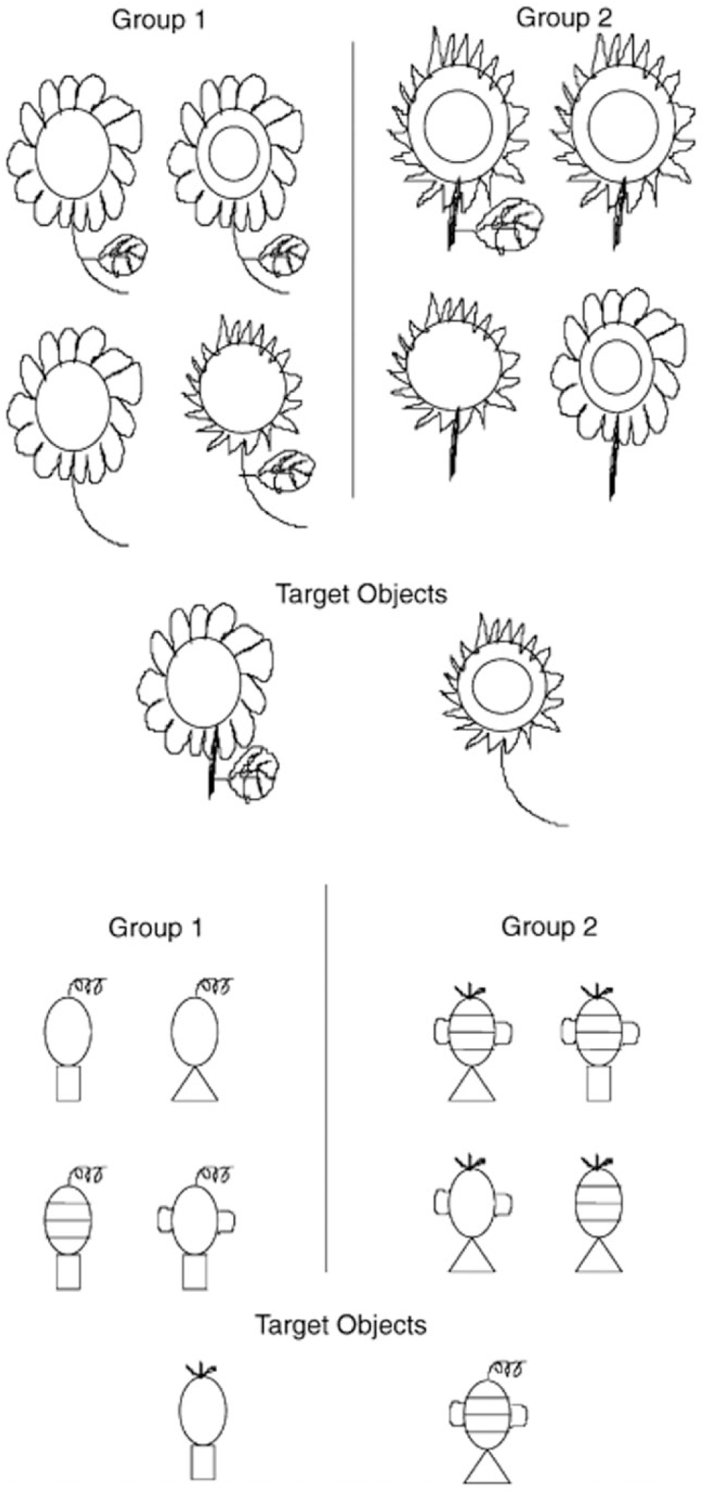
Examples of targets and groups used in the replication of Norenzayan, Smith, Kim, and Nisbett’s (2002) Study 2. Each of the two target objects in each set was presented separately with the two groups in order to achieve a counterbalanced design. For the flowers, the defining feature was the stem length; for the geometric figures, it was the topmost string.
Replication
For the replication, we preregistered a plan to compare the percentage of rule-based responses between the belong-to and similar-to conditions. In the original study, European Americans showed no difference between these conditions (d = 0.00, 95% CI = [−0.15, 0.15]), but East Asians were more likely to give rule-based responses in the belong-to condition than in the similar-to condition (d = 0.67, 95% CI = [0.52, 0.81). Note that we planned a comparison between the experimental conditions, whereas Norenzayan et al. (2002) focused their analysis and theoretical interest on comparisons between cultural groups within each experimental condition.
We computed the percentage of rule-based responses for each participant and then tested whether the mean percentages for the two experimental conditions were equal, using a t test for independent samples. In the aggregate replication sample (N = 7,396), participants who were asked “which group the target object belongs to” were more likely to classify on the basis of a rule (M = 64%, SD = 25%) than on the basis of family resemblance (M = 36%, SD = 25%), and participants who were asked “which group the target object is more similar to” were more likely to classify on the basis of family resemblance (M = 56%, SD = 21%) than on the basis of a rule (M = 44%, SD = 21%). The likelihood of using a rule was higher in the belong-to condition compared with the similar-to condition, t(7227.59) = 37.05, p = 3.04e−275, d = 0.86, 95% CI = [0.81, 0.91]. This pattern was in the same direction as the original aggregate result, and the effect size was somewhat larger: People were more likely to categorize on the basis of a rule when they considered what group the target belonged to and more likely to categorize on the basis of family resemblance when they considered what group the target was similar to. 5
Follow-up analyses
We identified a priori that this effect and the one reported by Tversky and Gati (1978) both involved similarity judgments and thus that the order of these study materials in Slate 2 might be particularly relevant. We tested whether Norenzayan et al.’s (2002) effect was moderated by whether its materials came before or after Tversky and Gati’s and observed very weak moderation by task order, t(7392) = 2.34, p = .02, d = 0.05, 95% CI = [0.01, 0.10].
21. Less-is-better effect (Hsee, 1998, Study 1)
Hsee (1998) demonstrated the less-is-better effect, wherein a less expensive gift can be perceived as more generous than a more expensive gift when the less expensive gift is a high-priced item compared with other items in its category, and the more expensive item is a low-priced item compared with other items in its category. In Hsee’s Study 1, 83 participants imagined that they were about to study abroad and had received a goodbye gift from a friend. In one condition, participants imagined receiving a $45 scarf bought in a store where the prices of scarves ranged from $5 to $50. In the other condition, participants imagined receiving a $55 coat bought in a store where the prices of coats ranged from $50 to $500. Participants in the scarf condition considered their gift giver significantly more generous (M = 5.63; scale from 0, not generous at all, to 6, extremely generous) than did those in the coat condition (M = 5.00), t(82) = 3.13, p = .002, d = 0.69, 95% CI = [0.24, 1.13], despite the gift being objectively less expensive.
In the replication, the dollar values were approximately adjusted for inflation. We converted the amounts to local currencies at sites where U.S. dollars would be relatively unfamiliar to participants. In the aggregate replication sample (N = 7,646), participants in the scarf condition considered their gift giver significantly more generous (M = 5.50, SD = 0.89) than did those in the coat condition (M = 4.61, SD = 1.34), t(6569.67) = 34.20, p = 4.5e−236, d = 0.78, 95% CI = [0.74, 0.83]. This result is consistent with the less-is-better effect, and the effect size was slightly larger than in the original demonstration (d = 0.78, 95% CI = [0.74, 0.83], vs. original d = 0.69).
22. Moral typecasting (Gray & Wegner, 2009, Study 1a)
Gray and Wegner (2009) examined the attribution of intentionality and responsibility as a function of perceived moral agency—the ability to direct and control one’s moral decisions. In their Study 1a, 69 participants read about an event involving a person high on moral agency (an adult man) and a person low on moral agency (a baby). In one condition, the man knocked over a tray of glasses, which resulted in harm to the baby. In the other condition, the baby knocked over the tray of glasses, which resulted in harm to the man. Participants then rated the degree to which the person who committed the act was responsible, how intentional the act was, and how much pain was felt by the victim (scales from 1 to 7). The adult man (M = 5.29, SD = 1.86) was evaluated as more responsible for committing the act than was the baby (M = 3.86, SD = 1.64), t(68) = 3.32, p = .001, d = 0.80, 95% CI = [0.31, 1.29]. Likewise, the adult man (M = 4.05, SD = 2.05) was rated as acting more intentionally than the baby (M = 3.07, SD = 1.55), t(68) = 2.20, p = .03, d = 0.53. Finally, when on the receiving end of the act, the adult man (M = 4.63, SD = 1.15) was viewed as feeling less pain compared with the baby (M = 5.76, SD = 1.55), t(68) = 3.49, p = .001, d = 0.85.
Replication
The effect of condition on perceived responsibility was identified as the primary relationship for replication. In the aggregate replication sample (N = 8,002), the adult man (M = 5.41, SD = 1.63) was evaluated as more responsible for committing the act than the baby (M = 3.77, SD = 1.79), t(7913.89) = 42.62, p < 3.32e−285, d = 0.95, 95% CI = [0.91, 1.00]. This result is consistent with the hypothesis that an adult’s perceived responsibility for harming a baby is greater than a baby’s perceived responsibility for harming an adult. The effect size in the replication was slightly larger than the original result (d = 0.95, 95% CI = [0.91, 1.00], vs. original d = 0.80).
Follow-up analyses
There were two additional dependent variables for secondary analysis: perceived intentionality and pain felt by the victim. The adult man (M = 3.62, SD = 1.89) was rated as acting more intentionally than the baby (M = 2.73, SD = 1.64), t(7864.62) = 22.51, p = 8.3e−109, d = 0.50, 95% CI = [0.46, 0.55]. And, when on the receiving end of the act, the adult man (M = 4.66 SD = 1.25) was viewed as feeling less pain compared with the baby (M = 5.44, SD = 1.25), t(7989) = 27.54, p = 1.5e−159, d = 0.62, 95% CI = [0.57, 0.66].
23. Moral violations and desire for cleansing (Zhong & Liljenquist, 2006, Study 2)
Zhong and Liljenquist (2006) investigated whether moral violations can induce a desire for cleansing. In their Study 2, under the guise of a study on the relationship between personality and handwriting, 27 participants hand-copied a first-person account of an ethical act (helping a coworker) or unethical act (sabotaging a coworker). Then, participants rated the desirability of five cleansing products and five noncleansing products (scale from 1, not at all, to 7, very much). Participants who copied the unethical account (M = 4.95, SD = 0.84) reported that the cleansing products were more desirable than did participants who copied the ethical account (M = 3.75, SD = 1.32), F(1, 25) = 6.99, p = .01, d = 1.02, 95% CI = [0.39, 2.44]. There was no difference between the unethical (M = 3.85, SD = 1.21) and ethical (M = 3.91, SD = 1.03) conditions in ratings of noncleansing products, F(1, 25) = 0.02, p = .89, d = 0.05.
Replication
The effect of interest for replication was whether condition affected ratings of the cleansing products. In the aggregate replication sample (N = 7,001), after participants who copied less than half of the first-person account were removed, participants who copied the unethical account (M = 3.95, SD = 1.43) and those who copied the ethical account (M = 3.95, SD = 1.45) rated the cleansing products as similarly desirable, t(6999) = −0.11, p = .91, d = 0.00, 95% CI = [−0.05, 0.04]. This result is not consistent with the hypothesis that copying an account of an unethical action increases the desirability of cleansing products compared with copying an account of an ethical action.
Follow-up analyses
The original study revealed no difference by condition in ratings of noncleansing products. In the replication, a 2 (condition) × 2 (type of product) linear mixed-effects model with participant as a random effect yielded no interaction, t(6999) = −0.57, p = .57, d = −0.01, 95% CI = [−0.06, 0.03]. Moreover, there was no difference between the ethical (M = 3.12, SD = 1.08) and unethical (M = 3.11, SD = 1.05) conditions in ratings of noncleansing products, t(6999) = 0.63, p = .53, d = 0.02, 95% CI = [−0.03, 0.06].
24. Assimilation and contrast effects in question sequences (Schwarz, Strack, & Mai, 1991, Study 1)
In this study, 100 participants answered a question about life satisfaction in a specific domain, “How satisfied are you with your relationship?” and a question about life satisfaction in general, “How satisfied are you with your life-as-a-whole?” Participants were randomly assigned to the order in which they answered the specific and general questions. When the specific question was asked first, the correlation between the responses to the two questions was strong (r = .67, p < .05). When the specific question was asked second, the correlation between the responses was weaker (r = .32, p < .05). The difference between these correlations was significant, z = 2.32, p < .01, q = 0.48, 95% CI = [0.07, 0.88].
The authors suggested that the specific-first condition made the relationship more accessible, so that participants were more likely to incorporate information about their relationship when evaluating their life satisfaction more generally. Because responses to the two items were linked by the accessibility of relationship information, they were correlated. In contrast, in the specific-second condition, relationship satisfaction was not necessarily accessible when participants evaluated their overall life satisfaction, so they could draw on any number of different areas to generate their response to the general question. Thus, the correlation between responses to the two items was weaker than in the specific-first condition.
Replication
In the aggregate replication sample (N = 7,460), when the specific question was asked first, the correlation between the responses to the two questions was moderate (r = .38). When the specific question was asked second, the correlation between the responses was slightly stronger (r = .44). The difference between these correlations was significant, z = −3.03, p = .002, q = −0.07, 95% CI = [−0.12, −0.02]. The replication effect was in the direction opposite that of the original effect, and the replication effect size was much smaller than the original result (q = −0.07, 95% CI = [−0.12, −0.02], vs. q = 0.48).
Follow-up analysis
In the original procedure, no other measures preceded the questions. This particular effect concerns the influence of question context, so it is reasonable to presume that task order will have an impact on it. Therefore, the data for the most direct comparison with the original were provided by the sites where this task was administered first in the slate. In that subsample (N = 470), when the specific question was asked first, the correlation between the responses to the two questions was strong (r = .41). When the specific question was asked second, the correlation between the responses was the same (r = .41). The difference between these correlations was not significant, z = 0.01, p = .99, q = 0.00, 95% CI = [−0.18, 0.18].
25. Effect of choosing versus rejecting on relative desirability (Shafir, 1993, Study 1)
In this study, 170 participants imagined that they were on the jury of a custody case and had to choose between two parents. One of the parents had both more strongly positive and more strongly negative characteristics (the extreme parent) than the other parent (the average parent). Participants were randomly assigned to either decide to award custody to one parent or decide to deny custody to one parent. Participants were more likely to both award (64%) and deny (55%) custody to the extreme parent than to the average parent, and the sum of these probabilities was significantly greater than 100%, z = 2.48, p = .013, d = 0.35, 95% CI = [−0.04, 0.68]. This finding was consistent with the hypothesis that negative features are weighted more strongly than positive features when people are rejecting options, and positive features are weighted more strongly than negative features when people are selecting options (Shafir, 1993).
In the aggregate replication sample (N = 7,901), participants were less likely to both award (45.5%) and deny (47.6%) custody to the extreme parent than to the average parent, and the sum of these probabilities (93%) was significantly smaller than the 100% one would expect if choosing and rejecting were complementary, z = −6.10, p = 1.1e−9, d = −0.13, 95% CI = [−0.18, −0.09]. This result was small in magnitude and in the direction opposite that of the original finding, and it is incompatible with the hypothesis that negative features are weighted more strongly when people are rejecting options and positive features are weighted more strongly when people are selecting options.
26. Priming “heat” increases belief in global warming (Zaval, Keenan, Johnson, & Weber, 2014, Study 3a)
Zaval et al. (2014) investigated how beliefs in climate change could be influenced by immediately available information about temperature. In their Study 3a, 300 Mechanical Turk workers reported their beliefs about global warming after completing one of three scrambled-sentence tasks; one task primed the concept of “heat,” another primed the concept of “cold,” and the third had no theme (control condition). There was a significant effect of condition on both belief in global warming, F(2, 288) = 3.88, p = .02, and concern about it, F(2, 288) = 4.74, p = .01, controlling for demographic and actual-temperature data. Post hoc pairwise comparisons revealed that on a 4-point scale (from 1, not at all convinced, to 4, completely convinced), participants in the heat-priming condition expressed stronger belief (M = 2.7, SD = 1.1) in global warming than did both participants in the cold-priming condition (M = 2.4, SD = 1.1), t(191) = 1.9, p = .06, d = 0.27, 95% CI = [0.05, 0.49], and participants in the control condition (M = 2.3, SD = 1.1), t(193) = 2.23, p = .03, d = 0.37, 95% CI = [0.14, 0.59]. Likewise, participants in the heat-priming condition expressed greater concern (M = 2.4, SD = 1.0) about global warming than did both participants in the cold-priming condition (M = 2.1, SD = 1.0; scale from 1, not at all worried, to 4, completely worried), t(191) = 2.15, p = .03, d = 0.31, 95% CI = [0.03, 0.59], and participants in the control condition (M = 2.1, SD = 1.0), t(193) = 2.23, p = .02, d = 0.31, 95% CI = [0.02, 0.59].
Replication
For the direct replication, the mean difference in concern about global warming between the heat- and cold-priming conditions was evaluated. In the aggregate replication sample, after participants who made errors in the sentence-unscrambling task were excluded (remaining N = 4,204), participants in the heat-priming condition (M = 2.47, SD = 0.90) and participants in the cold-priming condition (M = 2.50, SD = 0.89) expressed similar levels of concern about global warming, t(4202) = −1.09, p = .27, d = −0.03, 95% CI = [−0.09, 0.03]. This result is not consistent with the hypothesis that temperature priming alters concern about global warming. The effect was small, much weaker than the original finding, and in the opposite direction (d = −0.03, 95% CI = [−0.09, 0.03], vs. original d = 0.31).
Translations of the scrambled-sentence task may have disrupted the effectiveness of the manipulation. Therefore, the most direct comparison with the original effect size was provided by the sites where the test was administered in English only. In this subsample (N = 2,939), participants in the heat-priming condition (M = 2.40, SD = 0.90) also expressed similar concern about global warming compared with participants in the cold-priming condition (M = 2.44, SD = 0.89), t(2937) = −0.18, p = .24, d = −0.04, 95% CI = [−0.12, 0.03].
Follow-up analyses
Belief in global warming was included as a secondary dependent variable. In the aggregate replication sample (N = 4,212), participants in the heat-priming condition (M = 3.25, SD = 0.84) and participants in the cold-priming condition (M = 3.25, SD = 0.82) expressed similar belief in global warming, t(4210) = 0.50, p = .62, d = 0.00, 95% CI = [−0.06, 0.06]. In the subsample of participants who took the test in English, participants in the heat-priming condition (M = 3.25, SD = 0.86) and participants in the cold-priming condition (M = 3.23, SD = 0.85) also expressed similar belief in global warming, t(2940) = 1.40, p = .16, d = 0.02, 95% CI = [−0.05, 0.09]. Neither of these follow-up analyses was consistent with the original study’s finding that temperature priming influenced belief in global warming.
27. Perceived intentionality for side effects (Knobe, 2003, Study 1)
Knobe (2003) investigated whether helpful and harmful side effects are differentially perceived as being intended. Consider, for example, an agent who knows that his or her behavior will have a particular side effect, but does not care whether the side effect does or does not occur. If the agent chooses to go ahead with the behavior and the side effect occurs, do people believe that the agent brought about the side effect intentionally? Knobe had participants read vignettes about such situations and found that participants were more likely to believe the agent brought about the side effect intentionally when the side effect was harmful compared with when it was helpful. Eighty-two percent of participants in the harmful-side-effect condition said that the agent brought about the side effect intentionally, whereas 23% of those in the helpful-side-effect condition said that the agent brought about the side effect intentionally, χ2(1, N = 78) = 27.2, p < .001, d = 1.45, 95% CI = [0.79, 2.77]. Also, ratings of the blame deserved by agents who brought about harmful side effects were higher than ratings of the praise deserved by agents who brought about helpful side effects (scales from 1 to 7), t(120) = 8.4, p < .001, d = 1.55, 95% CI = [1.14, 1.95]. The total amount of blame or praise attributed to the agent was associated with belief that the agent brought about the side effect intentionally, r(120) = .53, p < .001, d = 0.63, 95% CI = [0.26, 0.99].
Replication
For the direct replication, ratings of intentionality in the harmful- and helpful-side-effect conditions were compared using a 7-point scale rather than a dichotomous judgment. In the aggregate replication sample (N = 7,982), participants in the harmful-side-effect condition (M = 5.34, SD =1.94) said that the agent brought about the side effect intentionally to a greater extent than did participants in the helpful-side-effect condition (M = 2.17, SD = 1.69), t(7843.86) = 78.11, p < 1.68e−305, d = 1.75, 95% CI = [1.70, 1.80]. This is consistent with the original result, and the effect was somewhat stronger in the replication (d = 1.75, 95% CI = [1.70, 1.80], vs. original d = 1.45).
Follow-up analyses
Blame and praise ratings were assessed as a secondary replication. Ratings of the blame deserved by agents who brought about harmful side effects were higher (M = 6.03, SD = 1.26) than ratings of the praise deserved by agents who brought about helpful side effects (M = 2.54, SD = 1.60), t(7553.82) = 108.15, p < 1.68e−305, d = 2.42, 95% CI = [2.36, 2.48]. This is also consistent with the original result, and the effect size is notably larger (2.42 vs. 1.55).
28. Directionality and similarity (Tversky & Gati, 1978, Study 2)
Tversky and Gati (1978) investigated the relationship between directionality and similarity. In their Study 2, 144 participants made 21 similarity ratings of country pairs in which one country (e.g., the United States) was shown in a pretest to be more prominent than the other (e.g., Mexico). In a between-participants manipulation, the pair was presented with either the more prominent country first (e.g., United States-Mexico) or the less prominent country first (e.g., Mexico-United States). Two counterbalanced versions of the survey were created such that the more prominent country and the less prominent country were presented first “about an equal number of times” (p. 87). Results indicated that participants’ similarity ratings were higher when less prominent countries were displayed first than when more prominent countries were displayed first, t(153) = 2.99, p = .003, d = 0.48, 95% CI = [0.16, 0.80], and that higher similarity ratings were given to the version of each pair that listed the more prominent country second, t(20) = 2.92, p = .001, d = 0.64, 95% CI = [0.16, 1.10].
A follow-up study (N = 46) with the same design examined ratings of differences rather than similarities. Results were consistent with the first study: Participants’ difference ratings were higher when the more prominent countries were displayed first than when the less prominent countries were displayed first, t(45) = 2.24, p < .05, d = 0.66, 95% CI = [0.06, 1.25], and higher difference ratings were given to the version of each pair that listed the more prominent country first, t(20) = 2.72, p < .01, d = 0.59, 95% CI = [0.12, 1.05].
Replication
For the replication, participants were randomly assigned to one of the two counterbalanced versions of the survey and were randomly assigned to rate either similarities or differences between the two countries in each pair. Following the design of the original studies, we considered the participants who provided similarity and difference judgments to be two independent samples. Therefore, each site had about half as much data for its critical test as for the tests of the other 27 effects. The similarity ratings were the primary focus for direct replication, and the difference ratings were examined in a secondary analysis.
For each participant in the aggregate similarities sample (N = 3,549), we created an asymmetry score, calculated as the average similarity rating when the prominent country appeared second minus the average similarity rating when the prominent country appeared first. Across participants, the asymmetry score was not different from zero, t(3548) = 0.60, p = .55, d = 0.01, 95% CI = [−0.02, 0.04]; the order of presentation of more and less prominent countries did not influence evaluations of their similarity. In addition, we observed that the average similarity ratings in one counterbalancing condition were 8.78 (SD = 2.44) and 8.84 (SD = 2.43) when the more prominent country was presented first and second, respectively, whereas the corresponding average similarity ratings in the other counterbalancing condition were higher, M = 10.14 (SD = 2.42) and M = 10.09 (SD = 2.44), respectively. In summary, there was no evidence of the key effect of country order (prominent country first vs. second), and similarity ratings were different between the counterbalancing conditions, a procedural effect.
Then, we reproduced the original by-item analysis. Participants’ similarity ratings were nearly identical when the less prominent country was displayed first (M = 9.42, SD = 2.61) and when the more prominent country was displayed first (M = 9.43, SD = 2.57), t(20) = −0.29, p = .78, d = −0.04, 95% CI = [−0.35, 0.26]. Thus, the overall replication effect size was near zero, and the effect was in the direction opposite the original findings.
Follow-up analyses
We conducted the same analyses on the difference ratings (N = 3,582). The asymmetry score was not different from zero, t(3581) = 1.70, p = .09, d = 0.03, 95% CI = [−0.004, 0.061]; the order of presentation of more and less prominent countries did not influence evaluations of their difference.
The by-item analysis showed that participant’s difference ratings were very similar when the more prominent country was displayed first (M = 11.19, SD = 2.54) compared with when the less prominent country was displayed first (M = 11.25, SD = 2.54), t(20) = 1.1, p = .29, d = 0.17, 95% CI = [−0.14, 0.47].
Order effects in general are reported in the Results section. As noted earlier, we identified a priori that this effect and Norenzayan et al.’s (2002) effect both involved similarity judgments and thus that the order of these study materials might be particularly relevant. We compared whether the asymmetry score for Tversky and Gati’s (1978) effect was moderated by whether the measures for Norenzayan et al.’s effect appeared before or after, and observed no moderation for the primary similarities test, t(3547) = −0.48, p = .63, d = −0.02, 95% CI = [−0.08, 0.05], or for the secondary differences test, t(3580) = −0.23, p = .82, d = −0.01, 95% CI = [−0.07, 0.06].
Results
For each of the 28 effects, Table 2 presents the original study’s effect size (with 95% CI), the median effect size for the replication samples, and the weighted mean of the replication effect sizes (with 95% CI) after pooling the data of all the samples. It also shows the percentage of samples in which the null hypothesis was rejected and the effect was in the expected direction, the percentage of samples in which the null hypothesis was rejected and the effect was in the unexpected direction, and the percentage of samples in which the null hypothesis was not rejected. The effects are ordered from the largest global replication effect size consistent with the original study, at the top of the table, to the largest opposite-direction effect, at the bottom. For original studies that had shown cultural differences, we present results separately for cultures with WEIRD scores above the mean (classified as “WEIRD” samples) and those with WEIRD scores below the mean (classified as “less WEIRD” samples), to avoid aggregating results when effects might be anticipated in some samples but not others (see the next section for an explanation of how WEIRD scores were calculated). (In these cases, the effects are ordered according to the global replication effect size in the WEIRD samples.) However, the differences observed between samples in the original research may not be expected to be replicated in our comparisons of aggregated cultural contexts. Therefore, we avoid drawing conclusions about replication of original cultural differences beyond what we have already discussed in reporting the findings for individual studies and what we discuss later in presenting our exploratory cultural comparisons.
Summary of Effect Sizes and Results of Significance Tests Across Replication Samples for Each of the 28 Effects
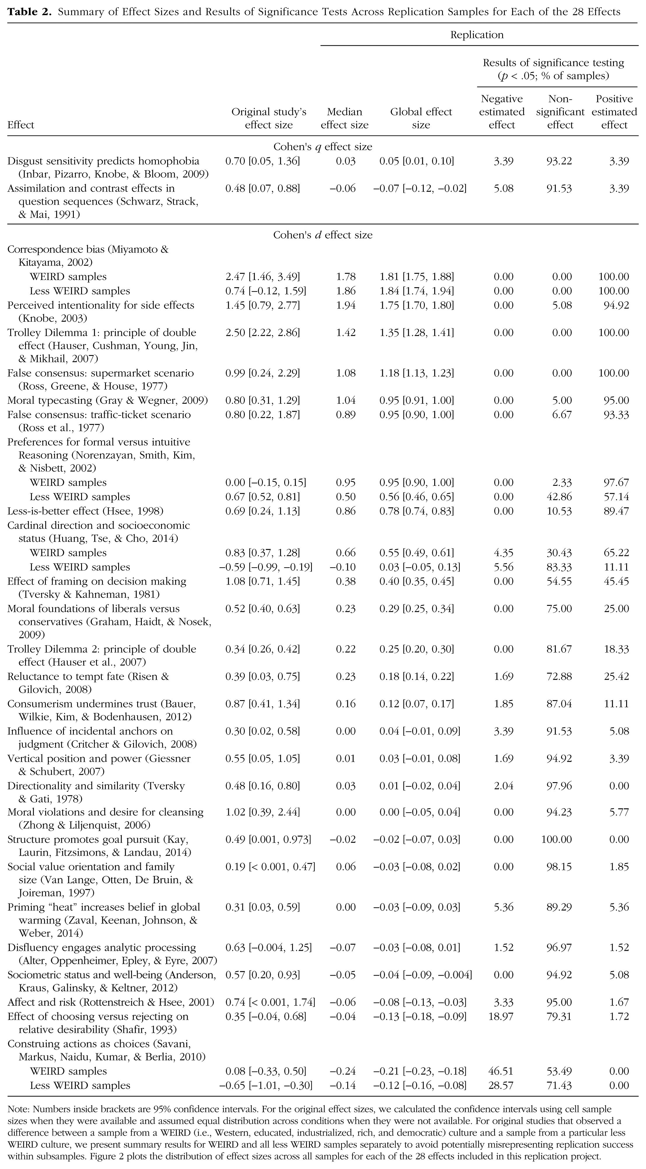
Note: Numbers inside brackets are 95% confidence intervals. For the original effect sizes, we calculated the confidence intervals using cell sample sizes when they were available and assumed equal distribution across conditions when they were not available. For original studies that observed a difference between a sample from a WEIRD (i.e., Western, educated, industrialized, rich, and democratic) culture and a sample from a particular less WEIRD culture, we present summary results for WEIRD and all less WEIRD samples separately to avoid potentially misrepresenting replication success within subsamples. Figure 2 plots the distribution of effect sizes across all samples for each of the 28 effects included in this replication project.
Overall, after we adjusted for multiple comparisons, the replications for 14 of the 28 effects (50%) showed significant evidence in the same direction as the original finding, 1 replication provided evidence that was weakly consistent with the original (4%), 6 and 13 replications (46%) yielded a null effect or evidence in the direction opposite the original finding. 7 Larger aggregate effects tended to have a higher percentage of significant positive results than smaller aggregate effects, as would be expected given the power of the individual samples to detect the observed aggregate effect size. For 8 of the supported effects, 89% to 100% of the individual samples had significant results, and for the other 6, 11% to 46% of the individual samples had significant results. As would be expected, for effects that were null in the aggregate, there were occasional significant results both in the original finding’s direction and in the opposite direction, but more than 90% of the individual samples typically showed a null effect. Most observed pooled effect sizes (21 of 28; 75%) were smaller than the original findings in WEIRD samples, but some (7 of 28; 25%) were larger.
Figure 2 provides a summary illustration of the 28 studies including (a) estimates of the aggregate effect sizes, (b) the effect-size estimate for each individual sample, and (c) the original studies’ effect-size estimates (results for samples from WEIRD and less WEIRD cultures are identified separately for the 4 original studies that had samples from two cultures). A figure showing separate distributions for WEIRD and less WEIRD replication samples is available in at https://osf.io/5yzn8/.
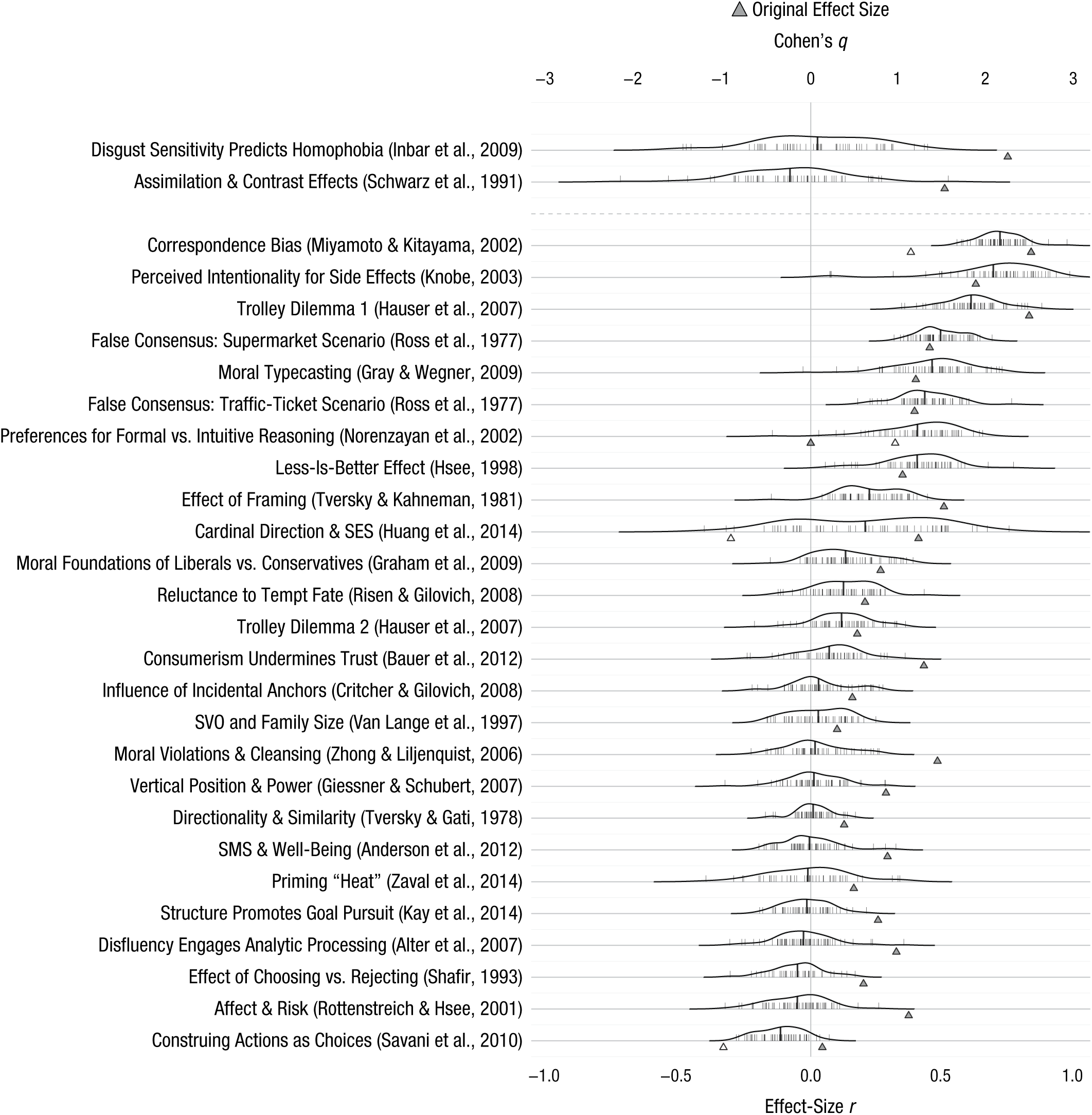
Effect-size distributions for the 28 effects. The effect size for each replication sample is plotted as a short vertical line; the aggregate estimates are plotted as longer, thick vertical lines. Results for samples with fewer than 15 participants because of exclusions are not plotted, and some samples were excluded because of errors in administration. A detailed accounting of all exclusions is available at https://manylabsopenscience.github.io/ML2_data_cleaning. Positive effect sizes indicate effects consistent with the direction of the original findings in the original Western samples. Original effect sizes are indicated by the gray-filled triangles. If the original study had a cultural comparison, the gray triangle shows the result for the WEIRD (Western, educated, industrialized, rich, and democratic) sample, and the open triangle shows the results for the less WEIRD sample. Note that for the top two rows of the figure, effect sizes were calculated as Cohen’s q (the estimate of the difference between two correlations); all other effect sizes were calculated as r. SES = socioeconomic status; SVO = social value orientation; SMS = sociometric status.
Variation across samples and settings
Our central interest was the variation in effect estimates across all samples and settings. In a linear mixed model with samples and studies as random effects, we compared the intraclass correlation (ICC) of samples across effects (ICC =.782), which was quite large, with the intraclass correlation of effects across samples (ICC = .004), which was near zero. In other words, to predict effect sizes across the 28 findings and dozens of samples studied in this project, it is very useful to know the effect in question and barely useful to know the sample in which it was being studied.
Next, we examined whether specific effects were sensitive to variation in sample or setting. For each of the 28 replication studies, we examined variability in effect sizes using a random-effects meta-analysis (with restricted maximum likelihood as the estimator for between-study variance) and established heterogeneity estimates—Q, I2, and tau—to determine if the amount of variability across samples exceeded that expected as a result of measurement error (see Table 3). Because the study procedures were nearly identical (except for language translations) across the individual studies, variation exceeding measurement error was likely to be due to effects of sample or setting and interactions between sample and materials. Eleven of the 28 effects (39%) showed significant heterogeneity according to the Q test (p < .001). Notably, of those showing such variability, the effect sizes for 8 were among the 10 largest effect sizes. Only one of the nonsignificant replication effects (i.e., replication of Van Lange et al., 1997) showed significant heterogeneity according to the Q test.
Results of Heterogeneity Tests for Each of the 28 Effects
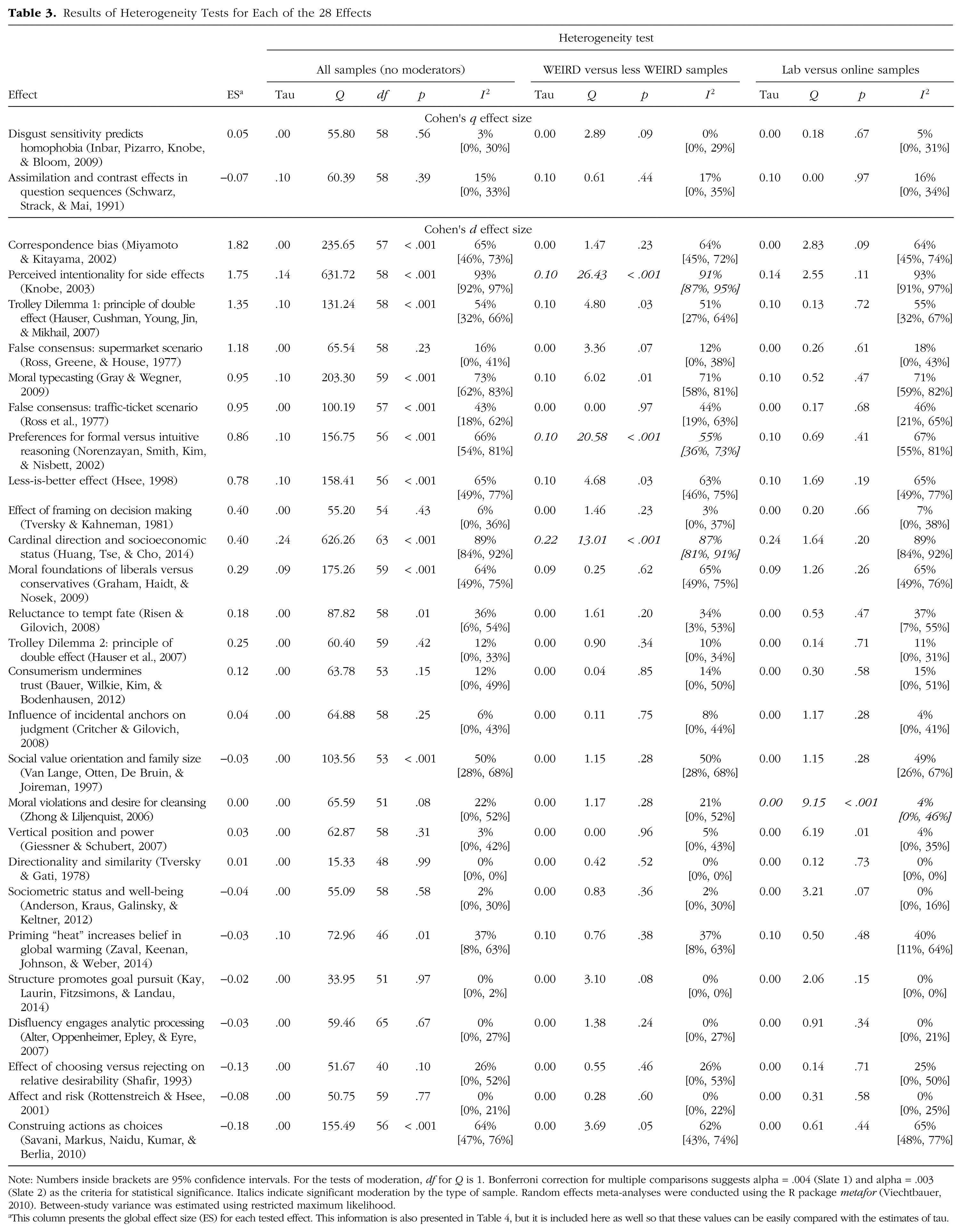
Note: Numbers inside brackets are 95% confidence intervals. For the tests of moderation, df for Q is 1. Bonferroni correction for multiple comparisons suggests alpha = .004 (Slate 1) and alpha = .003 (Slate 2) as the criteria for statistical significance. Italics indicate significant moderation by the type of sample. Random effects meta-analyses were conducted using the R package metafor (Viechtbauer, 2010). Between-study variance was estimated using restricted maximum likelihood.
This column presents the global effect size (ES) for each tested effect. This information is also presented in Table 4, but it is included here as well so that these values can be easily compared with the estimates of tau.
The I2 statistic indicated substantial heterogeneity for some of the tests; 10 (36%) showed at least medium heterogeneity (I2 ≥ 50%), and 2 showed heterogeneity larger than 75% (tests of Huang et al., 2014, and Knobe, 2003; see Table 3). Note, however, that estimation of heterogeneity is rather imprecise, as evidenced by the many large confidence intervals for I2, particularly for the cases with low estimates of heterogeneity. Fifteen I2 effects had a lower bound of 0%. Also, the I2 statistic increases if sample size increases, so the large samples in this project may explain the large I2 statistics that were observed (Rücker, Schwarzer, Carpenter, & Schumacher, 2008). As in the first Many Labs project (Klein et al., 2014a), heterogeneity was greater for large effects than for small effects. The Spearman rank-order correlation between aggregate effect size and I2 was .56.
Finally, as estimated with tau, only 1 effect (replication of Huang et al., 2014) showed substantial standard deviation among effect sizes (.24), and 8 others showed modest heterogeneity near .10. Most of the effects, 19 of 28 (68%), showed near zero heterogeneity as estimated by tau. Thus, according to this test, there was modest evidence of heterogeneity overall, and when it was observed in individual effects, it was quite small.
Table 3 summarizes the tests of moderation by lab versus online setting. After we adjusted for multiple comparisons, just one result showed a significant difference between lab and online samples (replication of Zhong & Liljenquist, 2006). For this effect, the overall result was not different from zero, and approximately 95% of the individual samples showed null effects. These results suggest the need for some caution in concluding that effects are moderated by whether data are collected in the lab or online.
For exploratory cultural comparisons, we computed a WEIRDness (Henrich et al., 2010) score for each sample based on its country of origin, using public country rankings. Western countries were given a score of 1, and Eastern countries were given a score of 0. Developed countries were given a score of 1, and emerging countries were given a score of 0. The list of developed countries was obtained from the United Nations (United Nations, Department of Economic and Social Affairs, Development Policy and Analysis Division, 2014). Scores for education, industrialization, and democratization were taken from the United Nations’ Education Index (Education Index, 2017) and Industrial Development Report (United Nations Industrial Development Organization, 2015) and from the Global Democracy Ranking (Campbell, Pölzlbauer, Barth, & Pölzlbauer, 2015). We then computed a global WEIRDness score for each sample by taking the mean across its scores. Details on the computation and specific links to the country rankings are available at https://osf.io/b7qrt/. Samples from countries with WEIRDness scores above the mean across samples were categorized as WEIRD (Slate 1: n = 42; Slate 2: n = 44), and samples from countries with WEIRDness scores below the mean were categorized as “less WEIRD” (Slate 1: n = 22; Slate 2: n = 17; see Fig. 3 for the distribution of WEIRDness scores).
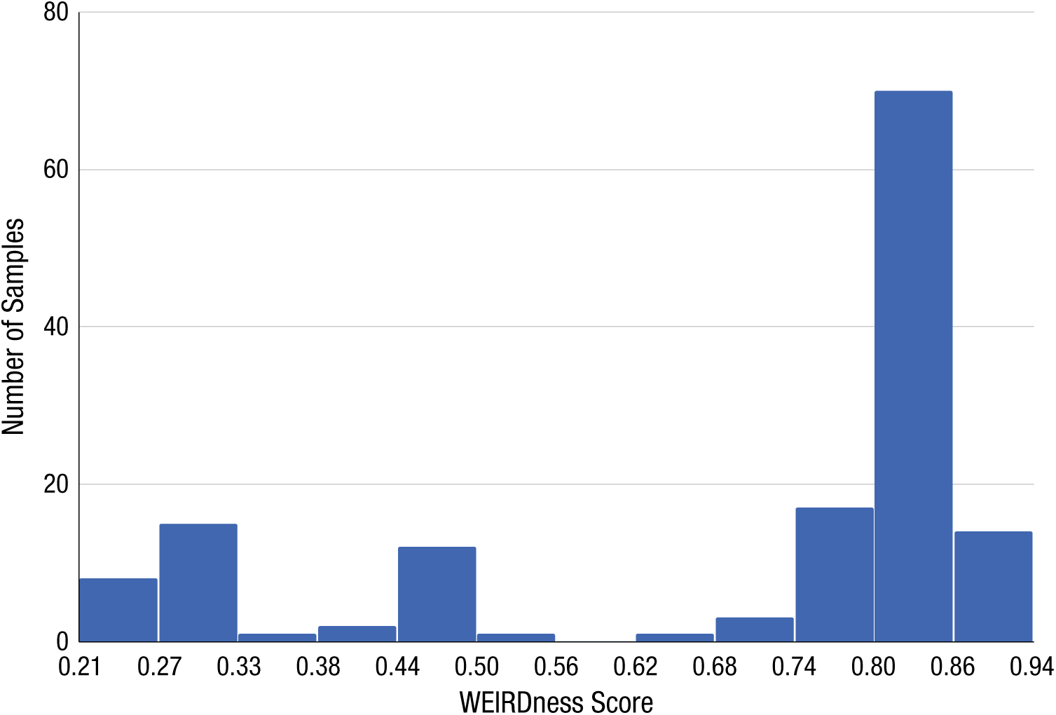
Histogram of the WEIRDness (Western, educated, industrialized, rich, democratic) scores of the samples.
Table 3 also presents heterogeneity statistics for comparisons of the WEIRD and less WEIRD cultures. For 13 of the 14 replication effects that were reliable and in the same direction as the effects in the original studies, the effect was observed with similar magnitude in the WEIRD and the less WEIRD samples. The only exception was Huang et al.’s (2014) effect; in this case, the WEIRD samples showed an effect in the same direction as the original WEIRD sample, and the less WEIRD samples showed no overall effect. Both showed wide variability across samples. This result is relatively consistent with the original study, in which Hong Kong and U.S. participants showed effects in opposite directions, presumably because of observed between-sample differences in whether wealthy people tended to live in the north or south. It is likely that there is wide variability in whether wealthy people tend to live in the north or south of the many different settings within our WEIRD and less WEIRD samples, and that this produced the high observed variability. Among the 14 effects that were null in the aggregate or in the direction opposite the effect in the original WEIRD sample, there was little evidence for the original finding in most WEIRD and less WEIRD samples. However, in the case of Savani et al.’s (2010) effect, both the WEIRD and the less WEIRD replication samples showed effects that were in the direction of the effect in the original Indian sample.
Ultimately, just three effects (those originally reported by Huang et al., 2014; Knobe, 2003; and Norenzayan et al., 2002) showed significant evidence for moderation by WEIRDness after correction for multiple comparisons. However, for Norenzayan et al.’s effect, the cultural difference was the inverse of the original result, though we note that the original study did not have a theoretical commitment regarding the cultural difference in the condition effect that we tested. Norenzayan et al. focused on rule-based responses across conditions and predicted that their European American sample would show greater rule-based responses than the East Asian sample within each condition (see note 5).
Influence of task order
The order in which tasks are presented could moderate effect sizes. Across a 30-min session, effects may weaken if participants tire or if earlier procedures interfere with later procedures. We did not observe this pattern in prior Many Labs investigations with the same design (Ebersole et al., 2016; Klein et al., 2014a), but task order remains a potential moderator. Order of administration in the current project was randomized, so we were able to test this possibility directly. Figure 4 shows the magnitude of each effect for each position in which it was presented in its slate (i.e., from 1, presented first, to 13 or 15, presented last). For each of the 28 effects, Table 4 shows the aggregate effect size, the effect size when the study was administered first, and the effect size when the study was administered last. Across the 28 findings, we observed little systematic evidence that effects were stronger (or weaker) when administered first compared with last. Also, there was no evidence of linear, quadratic, or cubic trends by task order (for analytic details, see https://osf.io/z8dqs/). Examination of all task positions for all 28 findings revealed that the aggregate effect size fell outside of the 95% CI for 29 of the 394 estimates (7.4%), a percentage that is not much different from what would be expected by chance (5%). Also, the distribution of the significant effects appears to have been relatively random across effects and positions (Fig. 4).
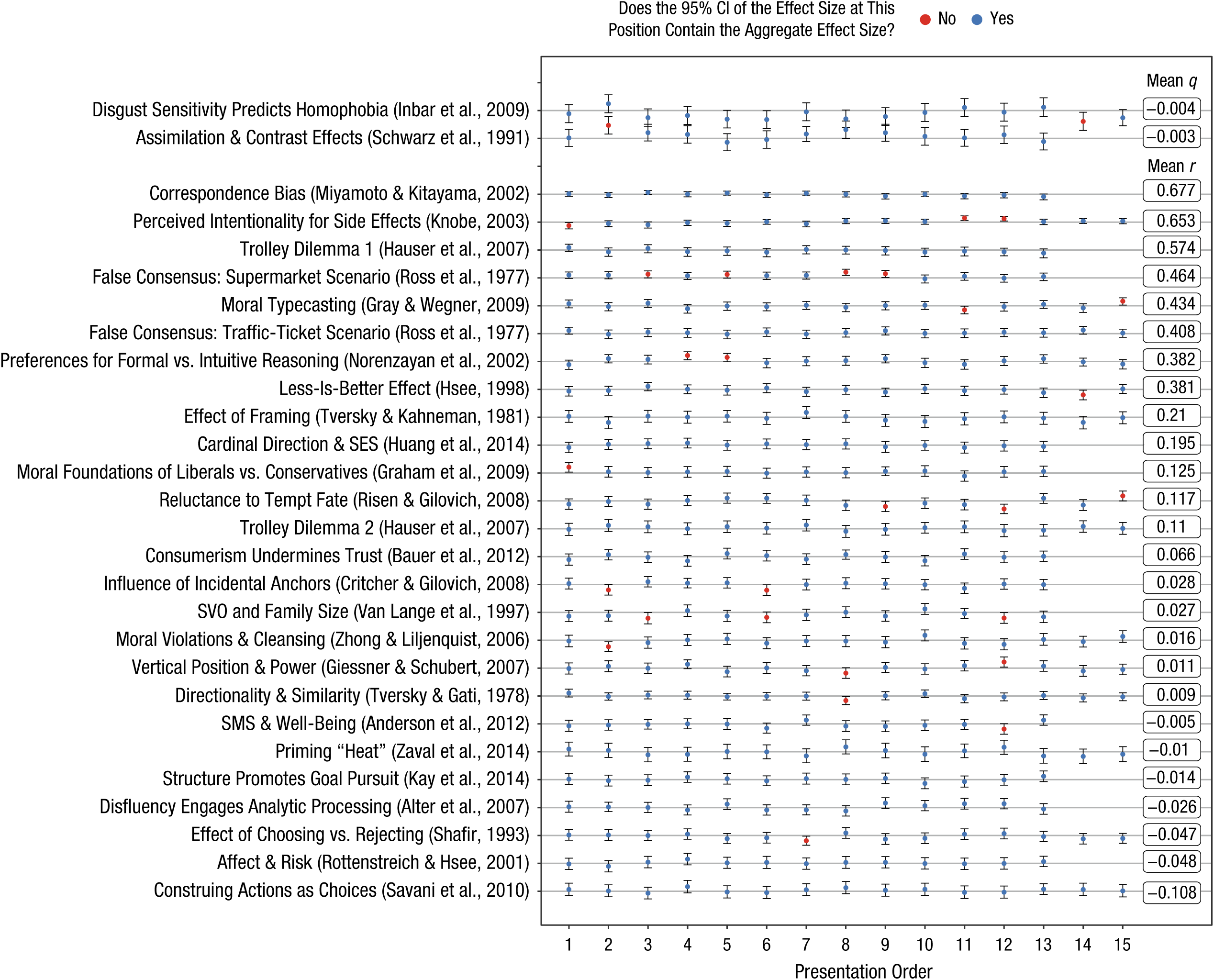
Effect-size estimates for each study for each position in which it was presented. For comparison, the aggregate effect size for each of the 28 effects is presented at the right. Error bars represent 95% confidence intervals (CIs). SES = socioeconomic status; SVO = social value orientation; SMS = sociometric status.
Comparison of Each Study’s Global Effect Size With Its Effect Size When the Study Was Administered First and Last in Its Slate
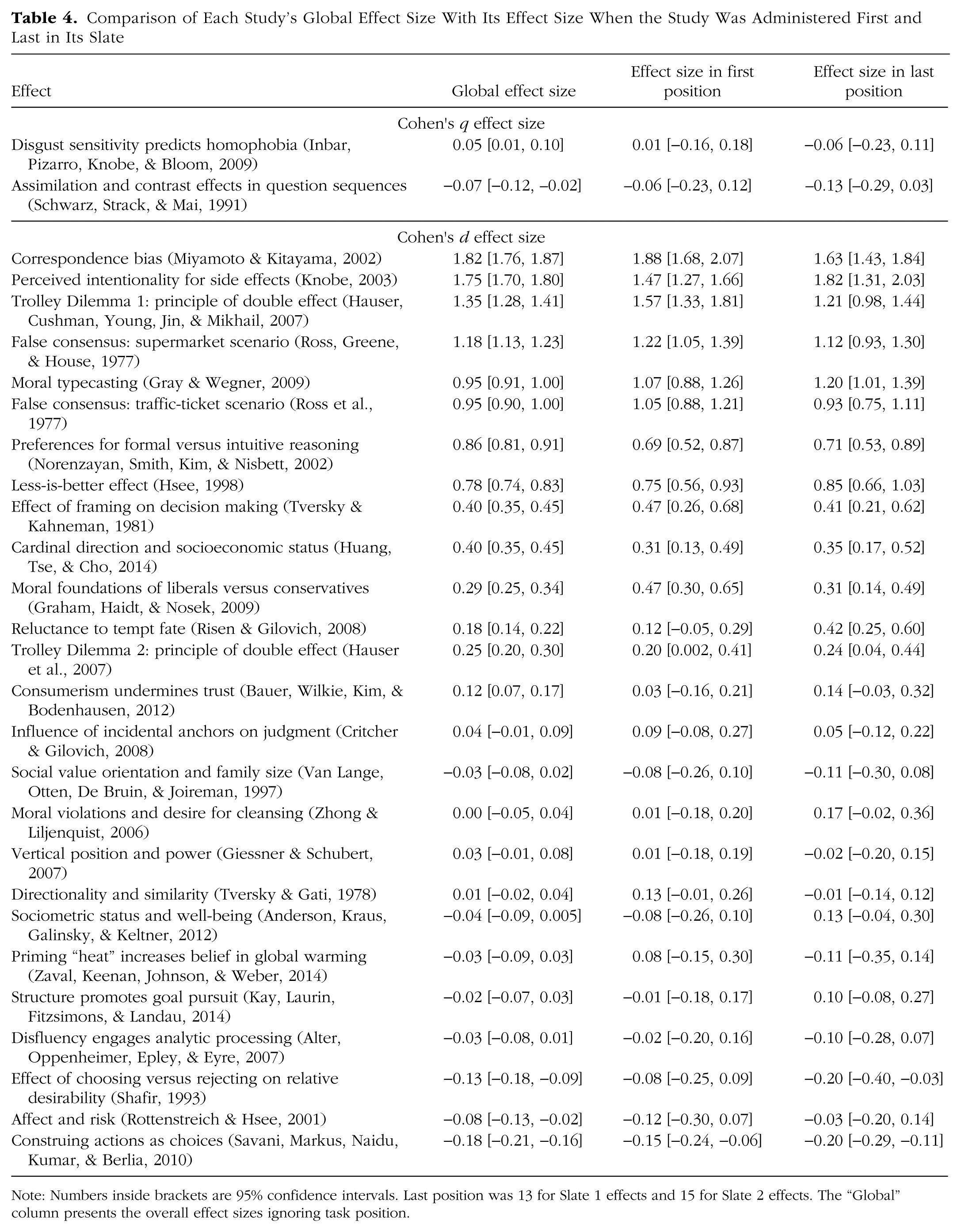
Note: Numbers inside brackets are 95% confidence intervals. Last position was 13 for Slate 1 effects and 15 for Slate 2 effects. The “Global” column presents the overall effect sizes ignoring task position.
Authors of four of the original articles (Alter et al., 2007; Giessner & Schubert, 2007; Miyamoto & Kitayama, 2002; Schwarz et al., 1991) noted a priori that their findings might be sensitive to order of administration. However, there was no evidence for systematic variation in magnitude by task order for any of these effects. It is still possible that there are specific order effects, such as when a particular procedure immediately precedes another particular procedure; but these analyses confirm that the findings, in the aggregate, are robust to task order and, particularly, that task order cannot account for observation of null effects for any of the nonreplicated results.
Discussion
With protocols that were peer reviewed in advance, we conducted preregistered replications of 28 published results, collecting data from 125 samples, including thousands of participants from locations around the world. According to the conventional criterion for statistical significance (p < .05), 15 (54%) of the replications provided significant evidence for an effect in the same direction as the original. According to a strict significance criterion (p < .0001), 14 (50%) of the 28 replications still provided such evidence—a reflection of the extremely high-powered design (for Inbar et al., 2009, the replication p value was .02). Seven (25%) of the replications had effect sizes (Cohen’s d or q) larger than the original, and 21 (75%) had effect sizes smaller than the original. In the WEIRD samples, the median Cohen’s d was 0.60 for the original findings and 0.15 for the replications—a substantial decline (Open Science Collaboration, 2015). 8 Sixteen replications (57%) had small effect sizes (< 0.20), and 9 (32%) replication effects were in the direction opposite that of the original finding. Three of the latter (i.e., replications of Rottenstreich & Hsee, 2001; Schwarz et al., 1991; and Shafir, 1993) had an aggregate replication effect size that was significantly in the opposite direction according to the p < .05 criterion, but only 1 (the replication of Shafir, 1993) was significant at the p < .0001 level.
There is no simple decision rule for declaring success or failure in replication or for detecting positive results (Benjamin et al., 2018; Camerer et al., 2018; Open Science Collaboration, 2015). In Table 5, we summarize the replication success for each of the 28 global effects according to five possible criteria. Each criterion evaluates whether the observed effect size would be considered statistically significant under different conditions. Two criteria used the replication data as reported in this article and applied either a loose significance criterion (p < .05) or a strict significance criterion (p < .0001). According to these criteria, the success rate was 54% or 50%, respectively. Other approaches considered what the p value would have been if the effect size we observed had been obtained with different sample sizes: the original study’s sample size, a sample 2.5 times the original study’s sample size (Simonsohn, 2015), or 50 participants per group—a reasonably large sample compared with historical trends (Fraley & Vazire, 2014). With the significance criterion set to p < .05 for all three cases, the success rate was 41%, 44%, or 35%, respectively. Ten of the effects (36%) were successfully replicated according to all the criteria that could be applied, and 13 (46%) were unsuccessfully replicated according to all the criteria that could be applied. 9 Five findings (18%) varied in replication success depending on the criterion used, usually because the replication effect size was substantially smaller than the original effect size.
Summary of Replication Success and Failure According to Different Criteria
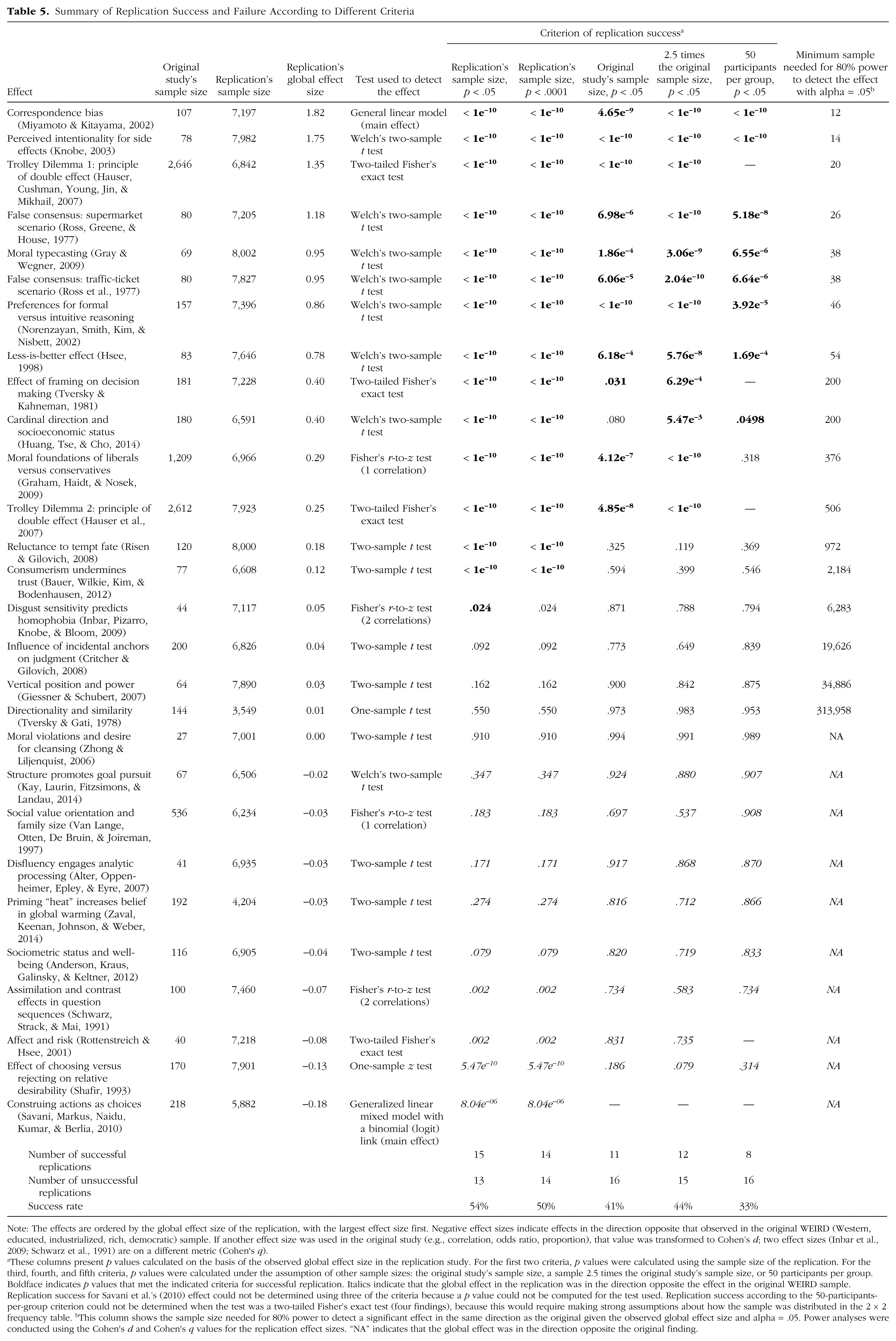
Note: The effects are ordered by the global effect size of the replication, with the largest effect size first. Negative effect sizes indicate effects in the direction opposite that observed in the original WEIRD (Western, educated, industrialized, rich, democratic) sample. If another effect size was used in the original study (e.g., correlation, odds ratio, proportion), that value was transformed to Cohen’s d; two effect sizes (Inbar et al., 2009; Schwarz et al., 1991) are on a different metric (Cohen’s q).
These columns present p values calculated on the basis of the observed global effect size in the replication study. For the first two criteria, p values were calculated using the sample size of the replication. For the third, fourth, and fifth criteria, p values were calculated under the assumption of other sample sizes: the original study’s sample size, a sample 2.5 times the original study’s sample size, or 50 participants per group. Boldface indicates p values that met the indicated criteria for successful replication. Italics indicate that the global effect in the replication was in the direction opposite the effect in the original WEIRD sample. Replication success for Savani et al.’s (2010) effect could not be determined using three of the criteria because a p value could not be computed for the test used. Replication success according to the 50-participants-per-group criterion could not be determined when the test was a two-tailed Fisher’s exact test (four findings), because this would require making strong assumptions about how the sample was distributed in the 2 × 2 frequency table. b This column shows the sample size needed for 80% power to detect a significant effect in the same direction as the original given the observed global effect size and alpha = .05. Power analyses were conducted using the Cohen’s d and Cohen’s q values for the replication effect sizes. “NA” indicates that the global effect was in the direction opposite the original finding.
The final column in Table 5 indicates the sample size that would be needed to have 80% power to detect each original effect given the observed global effect size and alpha of .05. Effects that were highly replicable across all the criteria were relatively large in magnitude and would be relatively efficient to investigate (i.e., they would require modest sample sizes: Ns from 12 to 54 except for one N of 200 and another of 506). Effects that were inconsistently replicated across criteria would need more substantial sample sizes to study efficiently (Ns from 200 to 2,184). Effects that were in the same direction as in the original study but too weak for us to reject the null hypothesis of no effect with our large samples would need massive samples to reject the null hypothesis (Ns from 6,283 to 313,958). Finally, for the 10 findings that had replication effect sizes of 0 or replication effects that were in the direction opposite the original, the null hypothesis cannot be rejected no matter what sample size is used.
The high proportion of failures to replicate, despite our extremely large samples, is consistent with the accumulating evidence from other systematic replication studies (Camerer et al., 2016; Camerer et al., 2018; Ebersole et al., 2016; Klein et al., 2014a; Open Science Collaboration, 2015). We cannot identify whether these results are due to errors in replication design, p-hacking in original studies, or publication bias in which positive results are selected despite pervasive low-powered research. However, it is notable that surveys and prediction markets in which researchers predicted and bet on whether these original effects would be replicated were effective at predicting replication success. For example, the correlation between market price and replication success for the Many Labs 2 studies was .755. These results are reported in a separate article (Forsell et al., in press) and replicate other studies using prediction markets and surveys to predict replication success (Camerer et al., 2016; Camerer et al., 2018; Dreber et al., 2016). In any case, these findings provide further justification for improving the transparency of research (Miguel et al., 2014; Nosek et al., 2015), preregistering studies to make all findings discoverable even if they are not published, and preregistering analysis plans to make clear the distinction between confirmatory tests and exploratory discoveries (Nosek, Ebersole, DeHaven, & Mellor, 2018; Wagenmakers, Wetzels, Borsboom, van der Maas, & Kievit, 2012).
The main purpose of this investigation was to assess variability in effect sizes by sample and setting. It is reasonable to expect that many psychological phenomena are moderated by variation in sample, setting, or procedural details, and that this variation may impact reproducibility (Henrich et al., 2010; Klein et al., 2014a, 2014b; Markus & Kitayama, 1991; Schwarz & Strack, 2014; Van Bavel, Mende-Siedlecki, Brady, & Reinero, 2016). However, we found a very strong correlation of samples across effects (ICC = .782), and we found a nearly zero correlation of effects across samples (ICC = .004). As one would expect, knowing the effect being studied provides much more information about effect size than does knowing the sample being studied. Just 11 of the 28 effects (39%) showed significant heterogeneity according to the Q test, and most of these 11 were among the effects with the largest overall magnitude. Only one of the near-zero replication effects (Van Lange et al., 1997) showed significant heterogeneity with the Q test. In other words, if no effect was observed overall, there was also very little evidence for heterogeneity among the samples.
The I 2 statistic indicated at least medium heterogeneity across samples for approximately one third of all the effects studied (36%), but almost all the I 2 estimates had high uncertainty (i.e., wide confidence intervals). Taken at face value, the I 2 statistics in Table 3 indicate that heterogeneity in the samples was high for some of the findings, even when there was little evidence for an effect. For example, for Zaval et al. (2014), the main effect was not distinguishable from zero, and 89% of the individual samples showed nonsignificant effects, which is close to expectation if the samples were drawn from a null distribution, and yet the I 2 was 37%. However, even if the average effect size is 0 and a majority of the results are null, there can be strong heterogeneity as measured with I 2 (see https://osf.io/frbuv/ for an explanation). I 2 compares variability in the dependent variable across samples with variability within samples. With increasing power, I 2 will tend toward 100% if there is any evidence for heterogeneity no matter how small the effect. Thus, our I 2 estimates likely reflect our extremely large sample sizes rather than the amount of heterogeneity in absolute terms.
By comparison, the estimates for tau in Table 3 indicate a small standard deviation in effect sizes for all studies except one (tau = .24 for Huang et al., 2014). In fact, 19 of the 28 effects (68%) had an estimated tau near 0, an indication of minimal heterogeneity, and 8 (29%) had an estimated tau near .10, an indication of a small amount of heterogeneity. It is not so surprising that this was the case for the effects that failed to be replicated globally, but it was also occasionally the case for successful replications. More important, even among the successful replications, when heterogeneity was observed with tau, it was relatively weak. As a consequence, at least for the variation investigated here, heterogeneity across samples does not provide much explanatory power for failures to replicate.
Our estimates of average effect size and effect-size heterogeneity may have been affected by imperfect reliabilities of the instruments that measured the outcome variables. For instance, Hunter and Schmidt (1990) showed how imperfect reliabilities attenuate effect-size estimates and suggested correcting for these imperfections when estimating effect size. As imperfect reliabilities were not corrected for in the original studies or our replications, systematic differences in effect-size estimates between the original and replication studies cannot be explained by imperfect reliabilities, unless the measurement instruments were systematically much less reliable in the replications than in the original studies; we have no evidence that this is the case. Differences across labs in reliabilities of measurement instruments may also result in overestimation of effect-size heterogeneity in cases of a true nonzero effect size. Insofar as these differences existed in the current investigation, our results likely overestimate heterogeneity, as our analyses did not take imperfect reliabilities of variables into account.
For 12 of the 28 effects, moderators or sample characteristics that may be necessary to observe the effect were identified a priori by the original authors or other experts during the Registered Report review process. These effect-specific analyses were reported in the section on the individual effects. For 7 of those 12, the pooled result was null or in the direction opposite the original; for the other 5, the pooled results showed evidence for the original finding. Evidence consistent with the hypothesized moderation was obtained for just 1 of the 12 effects (8% of the total; Hauser et al., 2007: Trolley Dilemma 1), and weak or partial evidence was obtained for 2 (17%; Miyamoto & Kitayama, 2002; Risen & Gilovich, 2008). For the other 9 (75%), there was little evidence that narrowing the data sets to the samples and settings deemed most relevant affected the likelihood of observing the effects or the original effect magnitudes. This does not mean that moderating effects do not occur, but it may mean that psychological theory is not yet advanced enough to predict them reliably.
Another possible moderating influence was task order. Participants completed their slate of 13 or 15 effects in a randomized order. It was possible that performance on tasks completed later in the sequence would be affected by tasks completed earlier in the sequence, either because of the specific content of the tasks or because of interference, fatigue, or other order-related influences (Ferguson, Carter, & Hassin, 2014; Kahneman, 2016; Schnall, 2014). Contrary to this prediction, we observed little evidence for systematic order effects for the 28 findings investigated. This replicates the lack of evidence for task-order effects observed in Many Labs 1 (Klein et al., 2014a) and Many Labs 3 (Ebersole et al., 2016). Across 51 total replication tests (28 reported here; 13 in Klein et al., 2014a; and 10 in Ebersole et al., 2016), we have observed little evidence for reliable effects of task order. The idea that whether a study comes first in a sequence, in the middle, or at the end has an impact on the magnitude of the observed effect is appealing but, so far, unsupported.
The same is true for effects of administration in lab versus online. Since the Internet became a source for behavioral research, there has been interest in the degree to which lab and online results are consistent with one another (Birnbaum, 2004; Dandurand, Shultz, & Onishi, 2008; Hilbig, 2016). As is the case for task order, across Many Labs projects we have observed little evidence for an effect of mode of administration. There may be conditions under which it is consequential whether a study is administered in the lab versus online, but we have not observed meaningful evidence for such an impact.
Finally, we included an exploratory analysis of the moderating influence of cultural differences between WEIRD and less WEIRD samples. We sampled from 125 highly heterogeneous sources (39 U.S. samples and 86 samples from 35 other countries and territories) to maximize the possibility of observing variation in effects based on sample characteristics. Ultimately, we found compelling evidence for differences between our WEIRD and less WEIRD samples for just three effects (those originally reported by Huang et al., 2014; Knobe, 2003; and Norenzayan et al., 2002).
However, our approach characterized cultural differences at the most general level possible—a dichotomy of WEIRDness—and ignored the rich diversity within that categorization. The distribution of WEIRDness scores was such that the WEIRD samples were highly similar in WEIRDness, and the less WEIRD samples varied substantially in WEIRDness. Figure 3 illustrates the highly skewed distribution. Countries with scores above 0.70 were categorized as WEIRD, and the rest were categorized as less WEIRD. Our summary analyses also did not address the possibility of highly specific regional variations, such as differences between U.S. and British samples, nor did they examine why differences were observed. Nor did these analyses investigate many interesting sampling moderators available in this data set, such as individual differences, gender, and ethnicity. Some moderating influences could be evaluated using the present data set; testing others will require new data collections. Also, a true examination of WEIRDness would need to more deliberately vary sampling across each of the WEIRD dimensions. Further analyses of the present data set may inspire hypotheses to be tested in future studies.
Implications
It is practically a truism that the human behavior observed in psychological studies is contingent on the cultural and personal characteristics of the participants under study and the setting in which they are studied. The depth with which this idea is embedded in present psychological theorizing is illustrated by the appeals to “hidden moderators” as explanations of failures to replicate when there have been no empirical tests of whether such moderators are operative (Baumeister & Vohs, 2016; Crisp, Miles, & Husnu, 2014; Gilbert, King, Pettigrew, & Wilson, 2016; Ramscar, Shaoul, & Baayen, 2015; Schwarz & Clore, 2016; Stroebe & Strack, 2014; Van Bavel et al., 2016). The present study suggests that dismissing failures to replicate as a consequence of such moderators without conducting independent tests of the hypothesized moderators is unwise. Collectively, we observed some evidence for effect-specific heterogeneity, particularly for relatively large effects; occasional evidence for cultural variation; and little evidence for moderation by procedural factors, such as task order and lab versus online administration.
There have been a variety of failures to replicate effects that were quite large in the original investigation (e.g., Doyen, Klein, Pichon, & Cleeremans, 2012; Hagger et al., 2016; Hawkins, Fitzgerald, & Nosek, 2015; Johnson, Cheung, & Donnellan, 2014). If effects are highly contingent on the sample and setting, then they could be large and easily detected in some samples and negligible in other samples. We did not observe this. Rather, evidence for moderation or heterogeneity was mostly observed in the large, consistently detectable effects.
Further, we observed some heterogeneity between samples, but a priori predictions (e.g., original authors’ predictions of moderating influences) and prior findings (e.g., previously observed cultural differences) were minimally successful in accounting for it. For the effects tested in Many Labs 2 at least, it appears that the cumulative evidence base has not yet matured enough for moderating influences to be predicted reliably. Simultaneously, there is accumulating evidence that researchers can predict the likelihood that an effect of interest will be replicated (Camerer et al., 2016; Camerer et al., 2018; Dreber et al., 2016; Forsell et al., in press).
For many multistudy investigations, a common template is to identify an effect in a first study and then report evidence for a variety of moderating influences in follow-up studies. A pessimistic interpretation would suggest that this template may be a consequence of practices that inflate the likelihood of false positives. Consider the context, in which positive results are perceived as more publishable than negative results (Greenwald, 1975) and common analytic practices may inadvertently increase the likelihood of obtaining false positives (Simmons et al., 2011). In a program of research, researchers might eventually obtain a significant result for a simple effect and call that Study 1. In follow-up studies, they might fail to observe the original effect and then initiate a search for moderators. Such post hoc searches necessarily increase the likelihood of false positives, but finding one may simultaneously reinforce belief in the original effect despite failure to replicate it. That is, identifying a moderator may feel like unpacking the phenomenon and explaining why the main effect “failed.”
An ironic consequence is that the identification of a moderator may simultaneously increase confidence in an effect and decrease its credibility. Investigating moderating influences is much harder than presently appreciated in practice. A 2 × 2 × 2 ANOVA has a nominal false positive rate of approximately .30 for one or more of its seven tests (1 – .957), yet correcting for multiple tests in multivariate analyses is rare (Cramer et al., 2016). Also, typical study designs are woefully underpowered for studying moderation (Frazier, Tix, & Barron, 2004; McClelland, 1997), perhaps because researchers intuitively overestimate the power of various research designs (Bakker, Hartgerink, Wicherts, & van der Maas, 2016). The combination of low power and lack of correction for multiple tests means that every study offers ample opportunity for “detecting” moderating influences that are not there.
Ultimately, the main implication of the present findings is a plain one: It is not sufficient to presume that moderating influences account for observed variation in a phenomenon. Cultural, sample, or procedural variation could be a reasonable hypothesis as an account for differences in observed effects, but it is not a credible hypothesis until it survives a confirmatory test (Nosek et al., 2018).
Limitations
The present study has the strength of data collected from very large samples from a wide variety of settings. Nevertheless, the generalizability of these results to other psychological findings is unknown. Fifty percent of the original effects we tested were reproduced, which is roughly consistent with the rate of replication success in other large-scale investigations (Camerer et al., 2016; Camerer et al., 2018; Ebersole et al., 2016; Klein et al., 2014a; Open Science Collaboration, 2015). However, the findings selected for this investigation were not a random sample of any definable population, nor did they constitute a large sample. It may be surprising that just 50% of the findings were reproduced under the circumstances of this project (original materials, peer review in advance, extremely high power, multiple samples), but that does not mean that 50% of all findings in psychology will be reproduced, or fail to be reproduced, under similar circumstances.
This study has the advantage over prior work by having included many tests and large samples, to achieve relatively precise estimation. Nevertheless, the failures to replicate do not necessarily mean that the tested hypotheses are incorrect. The lack of an effect may be limited to the particular procedural conditions of the test. Future theory and evidence will need to account for why the effects were not observed in these circumstances if they are replicable in others. Conversely, the successful replications add substantial precision for effect-size estimation and extend the generalizability of those phenomena across a variety of samples and settings.
Data availability
The amassed data set is very rich for exploring the individual effects, potential interactions between specific effects, and alternate ways to estimate heterogeneity and analyze the aggregate data. Our analysis plan focused on the big picture and not, for example, exploring potential moderating influences on each of the individual effects. These would be worthy analyses, but they are beyond the scope of a single report. Follow-up investigations using these data could provide substantial additional insight. For the accompanying Commentaries solicited by Advances in Methods and Practices in Psychological Science, we leveraged the extremely high-powered design of this study to demonstrate the productive interplay of exploratory and confirmatory analysis strategies. Commenters received a third of the data set for analysis. Upon completion of an exploratory analysis, the analytic scripts were registered and applied to the holdout data for a mostly confirmatory test (Nosek et al., 2018). The analysts’ decisions could have been influenced by advance observation of the summary results in this article, but use of the holdout sample reduced other potential biasing influences. Finally, the full data set (plus the portions used for the exploratory-confirmatory Commentaries) and all study materials are available at https://osf.io/8cd4r/ so that other teams can use them for their own investigations.
Conclusion
Our results suggest that variation across samples, settings, and procedures has modest explanatory power for understanding variation in the 28 effects included in this project. These results do not indicate that moderating influences never occur. Rather, they suggest that hypothesizing a moderator to account for observed differences in results between contexts is not equivalent to testing moderation with new data. The Many Labs paradigm allows testing across a broad range of contexts to probe the variability of psychological effects across samples. Such an approach is particularly valuable for understanding the extent to which given psychological findings represent general features of the human mind.
Supplemental Material
Klein_Open_Practices_Disclosure – Supplemental material for Many Labs 2: Investigating Variation in Replicability Across Samples and Settings
Supplemental material, Klein_Open_Practices_Disclosure for Many Labs 2: Investigating Variation in Replicability Across Samples and Settings by Richard A. Klein, Michelangelo Vianello, Fred Hasselman, Byron G. Adams, Reginald B. Adams, Sinan Alper, Mark Aveyard, Jordan R. Axt, Mayowa T. Babalola, Štěpán Bahník, Rishtee Batra, Mihály Berkics, Michael J. Bernstein, Daniel R. Berry, Olga Bialobrzeska, Evans Dami Binan, Konrad Bocian, Mark J. Brandt, Robert Busching, Anna Cabak Rédei, Huajian Cai, Fanny Cambier, Katarzyna Cantarero, Cheryl L. Carmichael, Francisco Ceric, Jesse Chandler, Jen-Ho Chang, Armand Chatard, Eva E. Chen, Winnee Cheong, David C. Cicero, Sharon Coen, Jennifer A. Coleman, Brian Collisson, Morgan A. Conway, Katherine S. Corker, Paul G. Curran, Fiery Cushman, Zubairu K. Dagona, Ilker Dalgar, Anna Dalla Rosa, William E. Davis, Maaike de Bruijn, Leander De Schutter, Thierry Devos, Marieke de Vries, Canay Doğulu, Nerisa Dozo, Kristin Nicole Dukes, Yarrow Dunham, Kevin Durrheim, Charles R. Ebersole, John E. Edlund, Anja Eller, Alexander Scott English, Carolyn Finck, Natalia Frankowska, Miguel-Ángel Freyre, Mike Friedman, Elisa Maria Galliani, Joshua C. Gandi, Tanuka Ghoshal, Steffen R. Giessner, Tripat Gill, Timo Gnambs, Ángel Gómez, Roberto González, Jesse Graham, Jon E. Grahe, Ivan Grahek, Eva G. T. Green, Kakul Hai, Matthew Haigh, Elizabeth L. Haines, Michael P. Hall, Marie E. Heffernan, Joshua A. Hicks, Petr Houdek, Jeffrey R. Huntsinger, Ho Phi Huynh, Hans IJzerman, Yoel Inbar, Åse H. Innes-Ker, William Jiménez-Leal, Melissa-Sue John, Jennifer A. Joy-Gaba, Roza G. Kamiloğlu, Heather Barry Kappes, Serdar Karabati, Haruna Karick, Victor N. Keller, Anna Kende, Nicolas Kervyn, Goran Knežević, Carrie Kovacs, Lacy E. Krueger, German Kurapov, Jamie Kurtz, Daniël Lakens, Ljiljana B. Lazarević, Carmel A. Levitan, Neil A. Lewis, Samuel Lins, Nikolette P. Lipsey, Joy E. Losee, Esther Maassen, Angela T. Maitner, Winfrida Malingumu, Robyn K. Mallett, Satia A. Marotta, Janko Međedović, Fernando Mena-Pacheco, Taciano L. Milfont, Wendy L. Morris, Sean C. Murphy, Andriy Myachykov, Nick Neave, Koen Neijenhuijs, Anthony J. Nelson, Félix Neto, Austin Lee Nichols, Aaron Ocampo, Susan L. O’Donnell, Haruka Oikawa, Masanori Oikawa, Elsie Ong, Gábor Orosz, Malgorzata Osowiecka, Grant Packard, Rolando Pérez-Sánchez, Boban Petrović, Ronaldo Pilati, Brad Pinter, Lysandra Podesta, Gabrielle Pogge, Monique M. H. Pollmann, Abraham M. Rutchick, Patricio Saavedra, Alexander K. Saeri, Erika Salomon, Kathleen Schmidt, Felix D. Schönbrodt, Maciej B. Sekerdej, David Sirlopú, Jeanine L. M. Skorinko, Michael A. Smith, Vanessa Smith-Castro, Karin C. H. J. Smolders, Agata Sobkow, Walter Sowden, Philipp Spachtholz, Manini Srivastava, Troy G. Steiner, Jeroen Stouten, Chris N. H. Street, Oskar K. Sundfelt, Stephanie Szeto, Ewa Szumowska, Andrew C. W. Tang, Norbert Tanzer, Morgan J. Tear, Jordan Theriault, Manuela Thomae, David Torres, Jakub Traczyk, Joshua M. Tybur, Adrienn Ujhelyi, Robbie C. M. van Aert, Marcel A. L. M. van Assen, Marije van der Hulst, Paul A. M. van Lange, Anna Elisabeth van ’t Veer, Alejandro Vásquez- Echeverría, Leigh Ann Vaughn, Alexandra Vázquez, Luis Diego Vega, Catherine Verniers, Mark Verschoor, Ingrid P. J. Voermans, Marek A. Vranka, Cheryl Welch, Aaron L. Wichman, Lisa A. Williams, Michael Wood, Julie A. Woodzicka, Marta K. Wronska, Liane Young, John M. Zelenski, Zeng Zhijia and Brian A. Nosek in Advances in Methods and Practices in Psychological Science
Footnotes
Appendix
Demographic, Data-Quality, and Individual Difference Measures, With Citation Counts
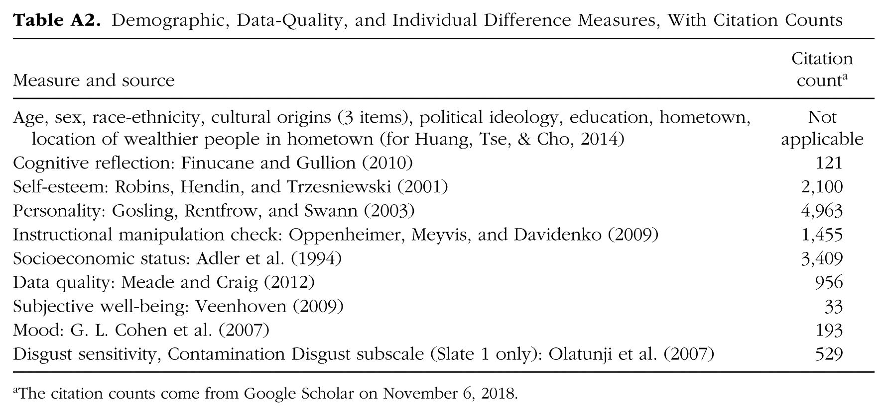
| Measure and source | Citation count a |
|---|---|
| Age, sex, race-ethnicity, cultural origins (3 items), political ideology, education, hometown, location of wealthier people in hometown (for Huang, Tse, & Cho, 2014) | Not applicable |
| Cognitive reflection: Finucane and Gullion (2010) | 121 |
| Self-esteem: Robins, Hendin, and Trzesniewski (2001) | 2,100 |
| Personality: Gosling, Rentfrow, and Swann (2003) | 4,963 |
| Instructional manipulation check: Oppenheimer, Meyvis, and Davidenko (2009) | 1,455 |
| Socioeconomic status: Adler et al. (1994) | 3,409 |
| Data quality: Meade and Craig (2012) | 956 |
| Subjective well-being: Veenhoven (2009) | 33 |
| Mood: G. L. Cohen et al. (2007) | 193 |
| Disgust sensitivity, Contamination Disgust subscale (Slate 1 only): Olatunji et al. (2007) | 529 |
The citation counts come from Google Scholar on November 6, 2018.
Acknowledgements
We thank Cameron Anderson, Adam Baimel, Galen Bodenhausen, Emma Buchtel, Zeynep Cemalcilar, Clayton Critcher, Itamar Gati, Kurt Gray, Christopher Hsee, Yanli Huang, Daniel Kahneman, Aaron Kay, Shinobu Kitayama, Joshua Knobe, Michael Kubovy, Yuri Miyamoto, Ara Norenzayan, Jane Risen, Lee Ross, Yuval Rottenstreich, Krishna Savani, Norbert Schwarz, Eldar Shafir, Chi-Shing Tse, Lisa Zaval, and Chen-Bo Zhong for helping develop and review materials, and for providing additional details from the original studies when needed.
Action Editor
Daniel J. Simons served as action editor for this article.
Author Contributions
F. Hasselman, R. A. Klein, B. A. Nosek, and M. Vianello coordinated the project. Š. Bahník, J. Chandler, K. S. Corker, F. Hasselman, H. IJzerman, R. A. Klein, B. A. Nosek, K. Schmidt, M. A. L. M. van Assen, L. A.Vaughn, M. Vianello, and A. L. Wichman designed the study. J. R. Axt, Š. Bahník, M. A. Conway, P. G. Curran, R. A. Klein, N. P. Lipsey, J. E. Losee, G. Pogge, and K. Schmidt developed the materials. J. R. Axt, Š. Bahník, M. Berkics, J. Chandler, E. E. Chen, S. Coen, M. A. Conway, K. S. Corker, W. E. Davis, T. Gnambs, F. Hasselman, H. IJzerman, R. A. Klein, C. A. Levitan, W. L. Morris, B. A. Nosek, K. Schmidt, V. Smith-Castro, J. Stouten, M. A. L. M. van Assen, L. A. Vaughn, M. Vianello, and A. L. Wichman wrote the proposal for the project. The data were collected by B. G. Adams, R. B. Adams, Jr., S. Alper, M. Aveyard, M. T. Babalola, Š. Bahník, R. Batra, M. Berkics, M. J. Bernstein, D. R. Berry, O. Bialobrzeska, E. D. Binan, K. Bocian, M. J. Brandt, R. Busching, A. Cabak Rédei, H. Cai, F. Cambier, K. Cantarero, C. L. Carmichael, F. Ceric, J. Chandler, J.-H. Chang, A. Chatard, E. E. Chen, W. Cheong, D. C. Cicero, S. Coen, J. A. Coleman, B. Collisson, K. S. Corker, P. G. Curran, F. Cushman, Z. K. Dagona, I. Dalgar, A. Dalla Rosa, W. E. Davis, M. de Bruijn, L. De Schutter, T. Devos, M. de Vries, C. Doğulu, N. Dozo, K. N. Dukes, Y. Dunham, K. Durrheim, C. R. Ebersole, J. E. Edlund, A. Eller, A. S. English, C. Finck, N. Frankowska, M.-Á. Freyre, M. Friedman, E. M. Galliani, J. C. Gandi, T. Ghoshal, S. R. Giessner, T. Gill, T. Gnambs, Á. Gómez, R. González, J. Graham, J. E. Grahe, I. Grahek, E. G. T. Green, K. Hai, M. Haigh, E. L. Haines, M. P. Hall, F. Hasselman, M. E. Heffernan, J. A. Hicks, P. Houdek, J. R. Huntsinger, H. P. Huynh, Hans IJzerman, Y. Inbar, Å. H. Innes-Ker, W. Jiménez-Leal, M.-S. John, J. A. Joy-Gaba, R. G. Kamiloğlu, H. B. Kappes, S. Karabati, H. Karick, V. N. Keller, A. Kende, N. Kervyn, R. A. Klein, G. Knežević, C. Kovacs, L. E. Krueger, G. Kurapov, J. Kurtz, D. Lakens, L. B. Lazarević, C. A. Levitan, N. A. Lewis, Jr., S. Lins, E. Maassen, A. T. Maitner, W. Malingumu, R. K. Mallett, S. A. Marotta, J. Međedović, F. Mena-Pacheco, T. L. Milfont, W. L. Morris, S. C. Murphy, A. Myachykov, N. Neave, K. Neijenhuijs, A. J. Nelson, F. Neto, A. L. Nichols, A. Ocampo, S. L. O’Donnell, H. Oikawa, M. Oikawa, E. Ong, G. Orosz, M. Osowiecka, G. Packard, R. Pérez-Sánchez, B. Petrović, R. Pilati, B. Pinter, L. Podesta, M. M. H. Pollmann, A. M. Rutchick, P. Saavedra, A. K. Saeri, E. Salomon, F. D. Schönbrodt, M. B. Sekerdej, D. Sirlopú, J. L. M. Skorinko, M. A. Smith, V. Smith-Castro, K. C. H. J. Smolders, A. Sobkow, W. Sowden, P. Spachtholz, M. Srivastava, T. G. Steiner, J. Stouten, C. N. H. Street, O. K. Sundfelt, S. Szeto, E. Szumowska, A. C. W. Tang, N. Tanzer, M. J. Tear, J. Theriault, M. Thomae, D. Torres, J. Traczyk, J. M. Tybur, A. Ujhelyi, R. C. M. van Aert, M. A. L. M. van Assen, M. van der Hulst, P. A. M. van Lange, A. E. van ’t Veer, A. Vásquez-Echeverría, L. A. Vaughn, A. Vázquez, L. D. Vega, C. Verniers, M. Verschoor, I. P. J. Voermans, M. A. Vranka, C. Welch, A. L. Wichman, L. A. Williams, M. Wood, J. A. Woodzicka, M. K. Wronska, L. Young, J. M. Zelenski, and Z. Zhijia. F. Hasselman, M. Vianello, and R. A. Klein analyzed the data, with support from K. S. Corker, B. A. Nosek, R. C. M. van Aert, and M. A. L. M. van Assen. F. Hasselman and B. A. Nosek designed the figures. R. A. Klein, B. A. Nosek, and M. Vianello wrote the report. All the authors commented on, edited, and approved the submitted manuscript.
Declaration of Conflicting Interests
Brian A. Nosek is Executive Director of the nonprofit Center for Open Science, which has a mission to increase openness, integrity, and reproducibility of research. The authors declared no additional potential conflicts of interest with respect to the authorship or the publication of this article.
Funding
This research was supported by the Center for Open Science and by a grant through the Association for Psychological Science from the Laura and John Arnold Foundation. The research in Chile was supported by Fondap Grant 15130009 from the Center for Social Conflict and Cohesion Studies.
Open Practices
All data and materials have been made publicly available via the Open Science Framework and can be accessed at https://osf.io/8cd4r/. The design and analysis plans were preregistered at the Open Science Framework and can be accessed at https://osf.io/c97pd/. The complete Open Practices Disclosure for this article can be found at http://journals.sagepub.com/doi/suppl/10.1177/2515245918810225. This article has received badges for Open Data, Open Materials, and Preregistration. More information about the Open Practices badges can be found at ![]() .
.
Notes
References
Supplementary Material
Please find the following supplemental material available below.
For Open Access articles published under a Creative Commons License, all supplemental material carries the same license as the article it is associated with.
For non-Open Access articles published, all supplemental material carries a non-exclusive license, and permission requests for re-use of supplemental material or any part of supplemental material shall be sent directly to the copyright owner as specified in the copyright notice associated with the article.