Sage Journals: Discover world-class research

Abstract

Hypothesis testing is a special form of model selection. Once a pair of competing models is fully defined, their definition immediately leads to a measure of how strongly each model supports the data. The ratio of their support is often called the likelihood ratio or the Bayes factor. Critical in the model-selection endeavor is the specification of the models. In the case of hypothesis testing, it is of the greatest importance that the researcher specify exactly what is meant by a “null” hypothesis as well as the alternative to which it is contrasted, and that these are suitable instantiations of theoretical positions. Here, we provide an overview of different instantiations of null and alternative hypotheses that can be useful in practice, but in all cases the inferential procedure is based on the same underlying method of likelihood comparison. An associated app can be found at https://osf.io/mvp53/. This article is the work of the authors and is reformatted from the original, which was published under a CC-By Attribution 4.0 International license and is available at https://psyarxiv.com/wmf3r/.

Keywords

Bayesian inference Bayesian statistics Bayes factor testing the null philosophy of science

Just as a computer stands ready to perform any calculation we ask of it, our present theory of Bayesian inference stands ready to answer any question we put to it.

—E. T. Jaynes (Rosenkrantz, 1983, p. 382)

The topic of this special section of Advances in Methods and Practices in Psychological Science is “providing evidence against the presence of a (meaningful) effect.” Here, we provide a few examples of how such evidence can be quantified. Once evidence is quantified, it can easily be combined with existing knowledge to evaluate the probability that an effect is (practically) nonexistent.

However, owing to the advancement of statistical computing power, it is not the computation of evidence or of probabilities that is most challenging in scientific inference. What is critical in the evaluation of theories, models, and hypotheses is that they are specified clearly and unambiguously. Indeed, once a model is sufficiently specified, the scientist only has to “turn the crank” of inference to calculate the evidence for or against the theory in question (Edwards, Lindman, & Savage, 1963). Both for quantifying evidence and for combining evidence with prior knowledge, researchers can turn to probability theory. The use of probability theory for scientific inference started with Bayes (1763), and subsequent seminal advances were contributed by de Finetti (1974), Jeffreys (1961), Laplace (1829), and Savage (1951). Several tutorials on Bayesian inference, including our most recent ones (Etz & Vandekerckhove, 2018, and Rouder & Morey, 2017), are available in the literature.

Here, we provide a theoretical introduction to the step that precedes these computational steps: stating a question clearly. We illustrate how slightly different questions can lead to different outcomes, and how models that seem qualitatively different are sometimes very difficult to distinguish statistically. In order to set up our discussion of precise scientific hypotheses, we first introduce some relevant concepts from the philosophy of science and statistics.

Occam’s Razor and Russell’s Teapot

It should be self-evident that no statistical procedure can discriminate between two models if they make exactly the same predictions for all scenarios (Wrinch & Jeffreys, 1921). Similarly, if one of the models is so flexible that it generates predictions that are arbitrarily close to the predictions of the other, they cannot be distinguished, strictly speaking. For example, if theory A says that some difference is 0 IQ points, theory B says the difference is 10^–12 IQ points, and modern studies have a maximum precision of roughly 5 points of difference, then intelligence researchers will simply have to make peace with the fact that IQ data alone cannot provide strong support for one theory over the other. If, on the other hand, theory C says that the difference can be anywhere from −100 to +100, and the available data happen to indicate that the difference is very close to zero, researchers are justified in concluding that the more complex, less parsimonious theory C should probably be discarded.

A famous argument by Bertrand Russell (1957) involves a mysterious teapot orbiting the Sun, somewhere between Earth and Mars. The argument can be summarized as follows: No observations that are available can conclusively rule out the existence of such a teapot—the “teapot theory” and the “no teapot theory” make essentially identical predictions about the data received by even the strongest telescopes.¹ However, the litany of additional assumptions that one would need in order to make the teapot theory likely is so extensive that any rational observer (justly) rejects the claim out of hand. The theory is not per se falsified by any data, but it lacks parsimony, and so with each observation that fails to confirm the existence of the teapot, evidence for its nonexistence accrues. Figure 1 provides a modern example of the same line of reasoning. This concept—that all other things being equal, simpler theories are preferred to more complex theories—is alternatively known as Occam’s razor, the principle of parsimony, and the simplicity rule (Myung & Pitt, 1997; Vandekerckhove, Matzke, & Wagenmakers, 2015).

Fig. 1.

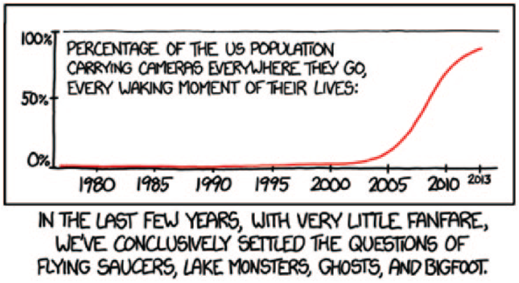
“Settled,” copyright 2014 by Randall Munroe (xkcd.com/1235). This comic makes the point that the existence of flying saucers and a number of unlikely creatures, such as lake monsters and Bigfoot, has gradually become falsified over the past decade or so as mobile cameras have become ubiquitous. The implication of this ubiquity is that if such creatures did exist, there is a high probability that clear photographic evidence of them would be available by now. By contrast, if they did not exist, any photographic evidence would be unclear and unconvincing, as it always has been. Given that clearer photographs have not emerged, and there are no strong prior reasons to believe in these phenomena, one may reasonably conclude that they do not exist. However, the jury is still out on the Grinch, Whos, and other snowflake dwellers.

Both of these insights from the philosophy of science—that some theories are impossible or impractical to distinguish from one another and that the more parsimonious explanation is preferable—are independently codified by probability theory, as we demonstrate in the remainder of this article.

Jeffreys’s Platitude

As cell-phone cameras have become more ubiquitous, the likelihood that Bigfoot exists has gradually dwindled. Similarly, as telescopes have grown more and more powerful, the existence of Russell’s teapot has gradually been falsified. However, an important realization about falsification claims is that the “mere existence” hypothesis is often underspecified. Suppose, for example, that Russell had specified that his teapot is approximately the size of Mars, and that it always resides close to that planet. This particularization of the teapot theory, though valid, is clearly falsified by the available data (because such an object would be visible to the naked eye). There is a clear distinction between the questions “Does the celestial teapot exist?” and “Does a celestial teapot with a volume of about 1.6 × 10¹¹ km³ exist?”

Jeffreys’s (1939) Platitude is, to paraphrase slightly, “Answers depend on questions.” In the context of statistical testing, it should be a platitude that if a researcher changes the definition of a statistical model, the evidence for or against this model may change as a result. Note that such model changes include changes in the prior knowledge regarding the values that parameters can and do take (such as the supposed volume of Russell’s teapot).

Statistical Inference

We have emphasized that the crux of inference is formulating the scientific question of primary interest. Once the question is formulated, the next step is to construct a statistical model to represent the scientific problem and identify the quantities of interest (e.g., what represents a “meaningful” or “practically relevant” effect?), before seeing how the data affect the probability of these quantities. Within the framework of Bayesian inference, this process is essentially automatic, following naturally from probability theory and Bayes’s famous theorem in particular.

We do not go into the finer details here (see Kass & Raftery, 1995, for a more detailed discussion) except to point out that in Bayesian inference, the probabilistic framework is used to update the prior probability of a theory (i.e., its plausibility before the data are seen) into its posterior probability (after the data are seen). The change in the relative probability of any two models after the data are observed is captured by the Bayes factor (Jeffreys, 1961). Specifically, when one is testing whether or not a meaningful effect exists, the Bayes factor (B) is

B = \frac{P (data | meaningful effect)}{P (data | no meaningful effect)} .

To obtain the posterior odds in favor of a meaningful effect, one multiplies the prior odds in favor of a meaningful effect with the Bayes factor (B):

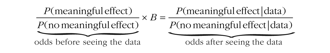
\underset{odds before seeing the data}{\underset{︸}{\frac{P (meaningful effect)}{P (no meaningful effect)}}} \times B = \underset{odds after seeing the data}{\underset{︸}{\frac{P (meaningful effect | data)}{P (no meaningful effect | data)}}}

If the Bayes factor is larger than 1, the data increase the odds in favor of the existence of a meaningful effect, and if the Bayes factor is less than 1, the data decrease these odds.

The Bayes factor updates the prior odds in favor of a meaningful effect to the posterior odds in favor of a meaningful effect by comparing the probabilities the two positions give to the observed data. In the following sections, we demonstrate how this comparison can be made across a number of scenarios, in which what constitutes a meaningful effect is determined primarily by context. We show that there is no such thing as “the” unique Bayes factor for any given data set: The Bayes factor expresses a relationship between the available data, on the one hand, and the question being asked, on the other (Morey & Rouder, 2011). As we argued earlier in the context of Jeffreys’s Platitude, it is both just and proper that the question being asked of the data affects the answer obtained, and one should be highly skeptical of any inferential method that ignores such important context.

Possible Scenarios

One way of putting Jeffreys’s Platitude in context is to draw a distinction between theoretical positions and model instantiations. A theoretical position is a verbal statement such as “there is no true effect” or “there is some true effect.” A model instantiation, or statistical hypothesis, takes a theoretical position and makes it sufficiently precise that it predicts where the data should occur before they are seen. The verbal statement “there is some true effect” fails this prediction test—on the basis of this statement, one cannot place a probability distribution over where the data are likely to occur. Rouder, Morey, and Wagenmakers (2016) noted that there are often many ways to instantiate hypotheses such as “there is no effect” or “there is some effect.” Jeffreys’s Platitude is a reminder that instantiations matter. Rouder et al. explored this important observation by positing that several research teams might instantiate different models of the existence of an effect. Here we expand that approach to the case in which one model specifies the presence of an effect and another specifies its absence.

Once competing models have been carefully constructed, one can activate the Bayesian machinery that makes it possible to determine how much evidence there is for each account. As has been argued elsewhere (e.g., Cox, 1946, Jaynes, 2003), probability theory is not merely one way of doing this but indeed is uniquely suited to it. The problem of assigning plausibility to competing hypotheses is solved exclusively by probability theory.

The point null hypothesis

Consider the popular example of “feeling the future” (Bem, 2011), or extrasensory perception (ESP). There are very specific hypotheses about what its nonexistence would look like. If ESP does not exist, there is not a smidgen of it. Performance on a chance task is at chance. The null hypothesis that accurately captures this account is a point null hypothesis. Under this hypothesis, the accuracy, θ, on a guessing task with two alternatives is exactly one half. We illustrate this hypothesis in Figure 2 (top panel) as a spike distribution (i.e., a vertical line).

Fig. 2.

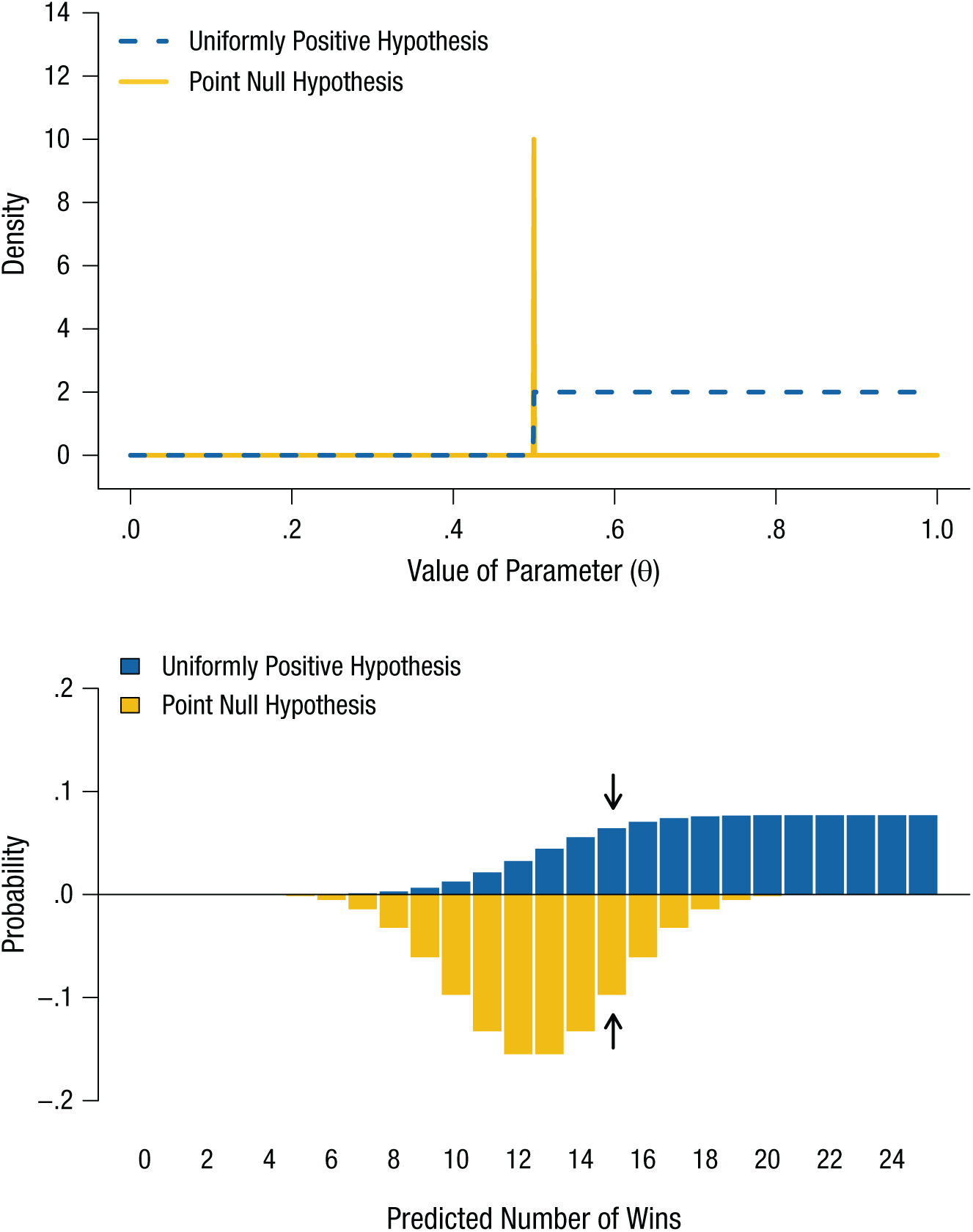
Illustration of competing point null and uniformly positive hypotheses regarding the existence of extrasensory perception, as applied to a binary guessing task. The probability densities of the two hypotheses are shown in the top panel. The point null hypothesis is represented by a spike at accuracy of .5, and the uniformly positive alternative spans from .5 to 1. The predictions of the two hypotheses are shown in the bottom panel; the Bayes factor is the ratio of the heights of the two bars for a given number of successes. The arrows highlight the probabilities of 15 successes out of 25 attempts. The Bayes factor given these data is approximately 1.51 in favor of the point null hypothesis.

What remains is to define an appropriate alternative with which this point hypothesis is to be compared. Here one runs into what might be called a teapot problem: Any amount of ESP would be a discovery for the ages, but just as it is impossible to devise an instrument that could detect a celestial teapot that is arbitrarily small, it is impossible to devise a test that can detect an arbitrarily small deviation in θ. Thus, the theoretical limits of inference have been reached. Now what?

One way to address this issue is to thoughtfully craft an alternative theoretical account informed by the specific context of the problem. In just the same way that a carefully devised null hypothesis can accurately capture what one thinks the absence of ESP should look like, an alternative that captures what ESP would look like, should it exist, can also be crafted.

The uniformly positive hypothesis

One possible conception of ESP is that a person who has it outperforms chance to some extent, but that all extents are equally likely. Under this alternative hypothesis, all values for θ that exceed one half are equally plausible, and all other values are ruled out. This uniformly positive hypothesis is shown in Figure 2 (top panel) as a uniform distribution from .5 to 1.

The Bayes Factor

Each of the two models now defined—the null hypothesis as a point and the alternative as an interval over one half of the range of possible values—implies a statement about what the data of some experiment would look like if the model were true. Suppose that we conducted some experiment on ESP with 25 trials with two choice options. Under the null hypothesis, in such an experiment there is approximately a .10 chance of being correct on 10 trials, a .13 chance of being correct on 11 trials, and so on (Fig. 2, bottom panel; see Box 1 for the prior and predictive distributions and the likelihood of 15 successes in 25 trials for each of the ESP hypotheses discussed in this article). Under the alternative hypothesis, these outcomes have a probability of only .01 and .02, respectively. Thus, statisticians might say that the null “predicts” or “expects” these outcomes more strongly than does the alternative, but it is important to note that this jargon has, for example, nothing to do with temporal order (i.e., a model can predict or expect observations that have occurred in the past), which is why some of the authors of this article prefer to refer to “support” for the data.

Box 1.

Definitions and Equations for the Models Introduced in the Text

For the purposes of statistical inference, a model is defined in sufficient detail if one can compute its predictive distribution P(data|H), that is, the probability of the data given the hypothesis. In our ESP example, the data are the number of wins k in a sequence of n trials, so that the predictive distribution is more precisely P_n(k | H).

The predictive distribution describes the relationship between the model and the data. Determining it is a matter of combining the relationship between the model and the parameter (i.e., the prior distribution of the parameter, θ, as defined by the model) with the relationship between the parameter and the data (i.e., the likelihood of the data given a particular value of θ). Per the sum rule of probability, the probability of getting k wins on n trials, given some hypothesis H is equal to the integral over the product of the likelihood and the prior:

P_{n} (k | H) = \int_{0}^{1} P (θ | H) P_{n} (k | θ) d θ .

Both components (the prior and the likelihood) are known for the models discussed in this article. Because the data are a number of wins, the likelihood is a Bernoulli distribution:

P_{n} (k | θ) = (\begin{matrix} n \\ k \end{matrix}) θ^{k} {(1 - θ)}^{n - k} .

The prior is unique to each model, and Table 1 presents each model’s prior and predictive distribution, along with the amount of support for each model given observed data of 15 wins out of 25 bets at the roulette table. These calculations and their background are covered in greater depth in Etz and Vandekerckhove (2018).

Table 1.

Model Equations for the Example Tests in the Article, With Predicted Probabilities of 15 Wins in 25 Bets at the Roulette Table

Hypothesis	Prior: p(θ \| H)	Predictive distribution: P_n(k \| H)	P₂₅(15 \| H)
Point null hypothesis	H₀: θ = .5	$(\begin{matrix} n \\ k \end{matrix}) {. 5}^{k} {(1 - . 5)}^{n - k}$	.0974
Competing-point hypothesis	H_A: θ = .53	$(\begin{matrix} n \\ k \end{matrix}) {. 53}^{k} {(1 - . 53)}^{n - k}$	.1257
Uniformly positive hypothesis	H₊: p(θ) = u(θ \| .5,1.0)	$\int_{0}^{1} u (θ \| . 5, 1.0) (\begin{matrix} n \\ k \end{matrix}) θ^{k} {(1 - θ)}^{n - k} d θ$	.0643
Uniformly negative hypothesis	H_–: p(θ) = u(θ \| .0,.5)	$\int_{0}^{1} u (θ \| . 0, . 5) (\begin{matrix} n \\ k \end{matrix}) θ^{k} {(1 - θ)}^{n - k} d θ$	.0126
Negligible-effect hypothesis	H_N: p(θ) = u(θ \| .47,.53)	$\int_{0}^{1} u (θ \| . 47, . 53) (\begin{matrix} n \\ k \end{matrix}) θ^{k} {(1 - θ)}^{n - k} d θ$	.0974
Nonnegligible-effect hypothesis	H_L: p(θ) = .5 × u(θ \| .0,.47) + .5 × u(θ \| .53,1.0)	$\int_{0}^{1} . 5 [u (θ \| . 0, . 47) + u (θ \| . 53, 1.0)] \times (\begin{matrix} n \\ k \end{matrix}) θ^{k} {(1 - θ)}^{n - k} d θ$	.0347
Slab hypothesis	H_S: p(θ) = u(θ \| .0,1.0)	$\int_{0}^{1} u (θ \| . 0, 1.0) (\begin{matrix} n \\ k \end{matrix}) θ^{k} {(1 - θ)}^{n - k} d θ$	.0385

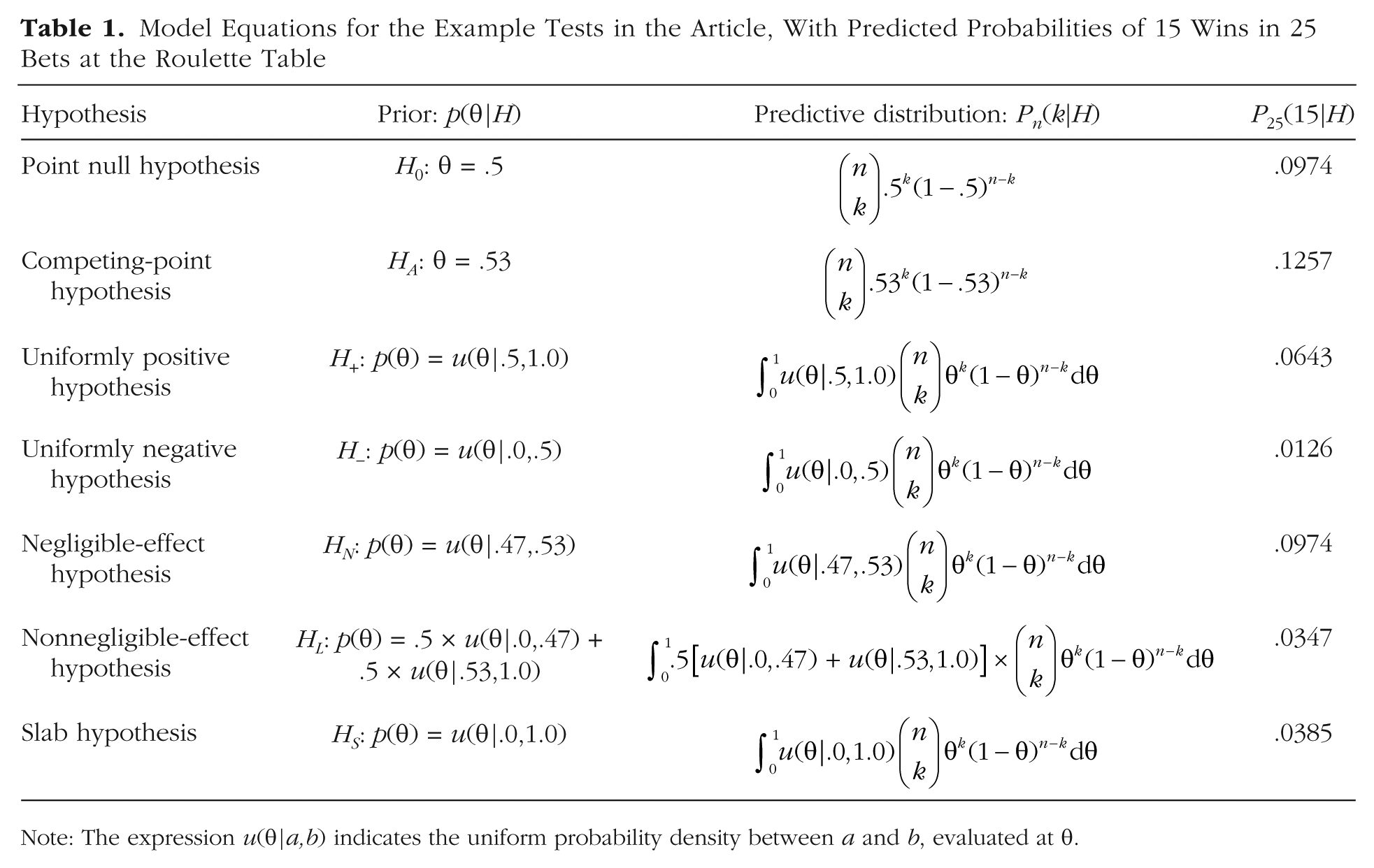
Note: The expression u(θ | a,b) indicates the uniform probability density between a and b, evaluated at θ.

The inference procedure consists of three steps. First, if possible, one determines the prior probability that the null hypothesis is true. For illustrative purposes, we assume equiprobability: that the prior odds are 1:1. Second, one uses the data to compute the Bayes factor. Third, one uses the Bayes factor to turn the prior odds into the posterior odds, by multiplying the prior odds with the Bayes factor.

Direct computation of the Bayes factor can be challenging when dealing with complicated models, often requiring numerical approximation, but conceptually the Bayes factor is always the relative strength with which the observed data were expected under each model. Suppose, for example, that a participant in our experiment got 15 of the 25 answers correct. The point null hypothesis gives this outcome a .0974 probability, whereas the alternative hypothesis gives it only a .0643 probability (see the arrows in the bottom panel of Fig. 2), so the Bayes factor is 1.51 (.0974/.0643) in favor of the null. Multiplying 1.51 with the prior odds of 1:1 gives posterior odds of 1.51:1, or a posterior probability on the null hypothesis of just above .60.

Other Possible Scenarios

We cannot emphasize enough the importance of Jeffreys’s Platitude to the practice of model selection (and hypothesis testing). To illustrate this point, in this section we discuss additional conceptualizations of the presence and absence of effects.

The competing-point hypothesis

The simplest bet in a game of American roulette is to pick one color (e.g., red). The odds of winning this bet are 18:20 (there are 18 red pockets, 18 black pockets, and 2 green pockets), so there is approximately a .53 chance of losing. The .03 difference from parity is called the house advantage, which is created by the carefully controlled way in which casinos “stack the deck” to ensure profit. Suppose that we think that, if ESP exists, it gives the clairvoyant a subtle edge at roulette—just enough to give the clairvoyant the .03 advantage over parity. We might now say that this .53 chance is the magnitude at which we expect ESP to be expressed in our data. Thus, we now have the most informative alternative hypothesis possible: an exact specification of θ.

The top panel in Figure 3 shows the probability densities for this competing-point hypothesis and the point null hypothesis, and the associated predictions about the data are displayed in the bottom panel as two histograms. One salient feature of these histograms is that they are very similar. The Bayes factor in favor of the competing-point hypothesis given 15 wins in 25 bets (highlighted by the arrows in Fig. 3) is small—a mere 1.29 (.1257/.0974)—and even at the very extreme ends of the possible observations (0 and 25 wins out of 25 bets), the support for the two hypotheses differs at most by a factor of 4.7. That is, even the most diagnostic data set of 25 observations imaginable would not deliver very much evidence to discriminate between these two accounts. We have another teapot problem and need to gather more data (if we really do care about distinguishing between two so similar hypotheses).

Fig. 3.

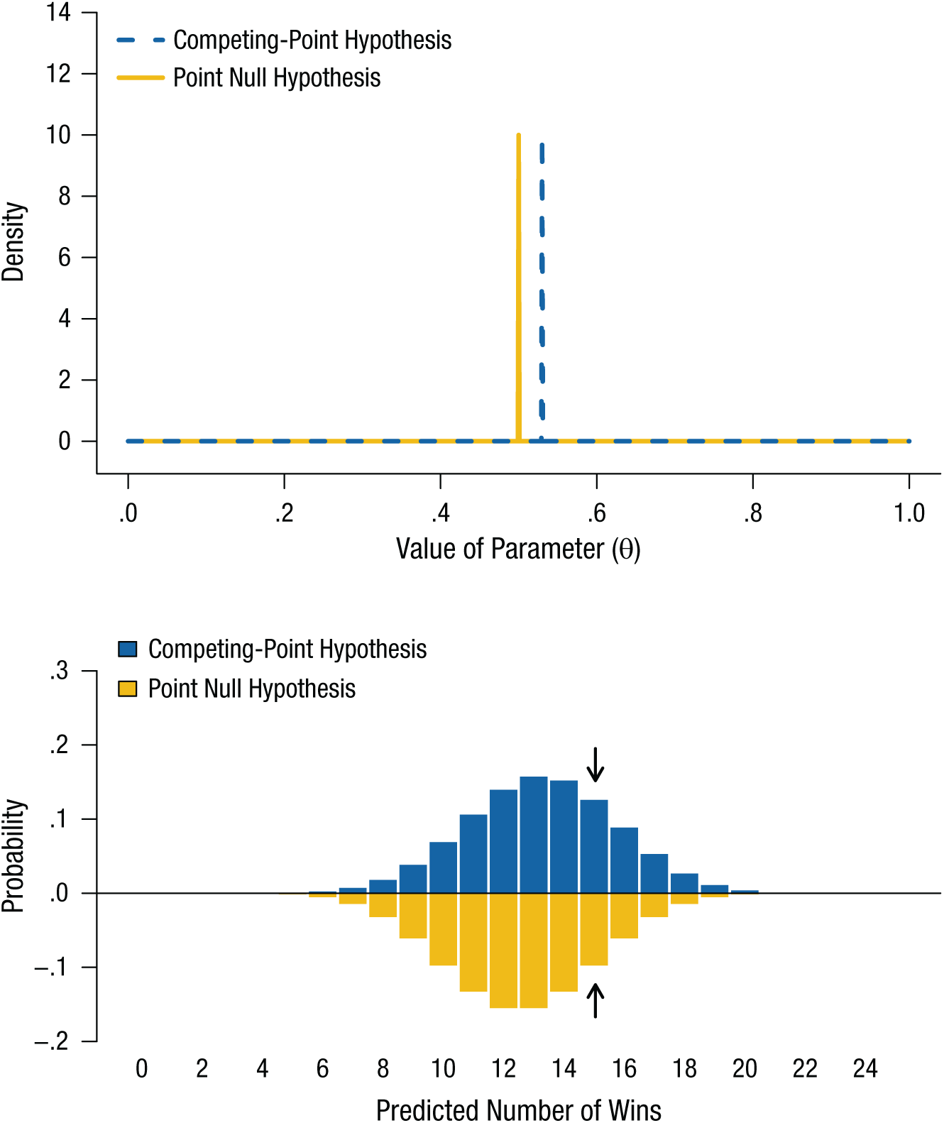
Illustration of point null and competing-point hypotheses regarding the existence of extrasensory perception, as applied to betting at roulette. The probability densities of the two hypotheses are shown in the top panel. The point null hypothesis is represented by a spike at accuracy of .50, and the competing-point hypothesis is represented by a spike at accuracy of .53. The predictions of the two hypotheses are shown in the bottom panel; the Bayes factor is the ratio of the heights of the two bars for a given number of wins. Note that because the predictions are hard to distinguish, it is not possible to obtain much evidence for one hypothesis over the other. The arrows highlight the predicted probabilities of 15 successes out of 25 attempts.

The positive-decay hypothesis

Rouder, Morey, and Province (2013) instantiated the “there is some effect” position with a hypothesis stipulating that if ESP exists, people should outperform chance, but that different levels of better-than-chance performance have different probabilities. More specifically, according to this hypothesis, higher performance levels have lower probabilities, so that .51 is more likely than .52, and so on. This is a flexible hypothesis, which allows for all possible values that are greater than chance, but prioritizes small effects over larger ones. Because they believed that this hypothesis made reasonable commitments, Rouder et al. emphasized this positive-decay hypothesis in their meta-analysis of ESP effects.

The negligible-effect hypothesis

A researcher may also choose different instantiations of the null position. Another aspect of statistical inference that is often neglected is the practical significance of an effect. Suppose that the goal is not simply to establish that ESP exists, but rather to monetize future telling at a casino—for example, at the roulette table. In order to reliably outperform the house, gamblers who bet according to their predictions would have to be at least 53% accurate. However, clever gamblers who are reliably less than 47% accurate in their predictions can also outperform the house if they simply play the color opposite the one they predict.

These observations suggest a new instantiation of the null hypothesis that does not, strictly speaking, say that ESP does not exist, but says merely that its effect is negligible for practical purposes. Such a hypothesis involves what is often called an equivalence region (Rogers, Howard, & Vessey, 1993), and it can be tested with exactly the same procedure as before. First, one defines the smallest nonnegligible departure from chance, which in this case is .03, and uses that value to define the negligible-effect hypothesis. In this case, this hypothesis states that only values of θ between .47 and .53 are plausible (i.e., the equivalence region has a width of .06). Next, one defines a complementary nonnegligible-effect hypothesis, which consists of two regions: in this case, 0 to .47 and .53 to 1.0.

The comparison of these two hypotheses is displayed in Figure 4, which shows more clearly an interesting effect that was less obvious in the previous examples. Because the nonnegligible-effect hypothesis is quite vague—it states that θ can take any value that is sufficiently far away from .50 (see the top panel)—and because the total probability that anything happens has to remain exactly 1, the strength of prediction of each individual outcome (bottom panel) is quite low. That is, to accommodate all the possible outcomes, the model is spread very thin, and there is no strong prediction anywhere.

Fig. 4.

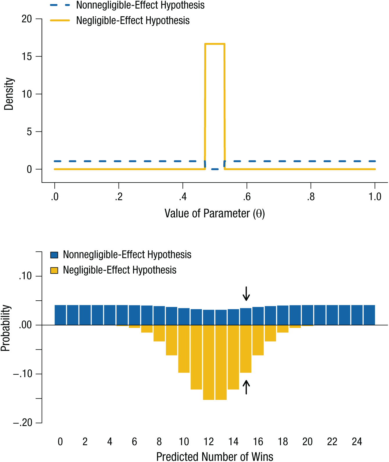
Illustration of negligible-effect and nonnegligible-effect hypotheses regarding the existence of extrasensory perception, as applied to betting at roulette. The probability densities of the two hypotheses are shown in the top panel. The negligible-effect hypothesis is represented by a null interval centered on a probability of .5, and the nonnegligible-effect hypothesis is represented by its complement. The predictions of the two hypotheses are shown in the bottom panel; the Bayes factor is the ratio of the heights of the two bars for a given number of wins. The arrows highlight the predicted probabilities of 15 successes out of 25 attempts. Because the nonnegligible-effect hypothesis spreads its predictions thinly over the space of possible outcomes, the more parsimonious negligible-effect hypothesis has the stronger support given these data.

The fact that every model has the same fixed amount of probability to assign to the possible outcomes leads to an automatic penalty for models that hedge over many different possibilities. This penalty for model freedom is a direct and unavoidable consequence of probability theory, and is a formal implementation of Occam’s razor.

As the bars highlighted by arrows in Figure 4 show, the Bayes factor favoring the negligible-effect hypothesis is about 2.8 if a roulette player wins 15 out of 25 times. If the prior odds were equal, this outcome means that the posterior probability favoring the negligible effect is about .74.

The spike-and-slab comparison

Scientists are often interested in knowing if there is any effect as opposed to no effect. Thus, one particularly common and tempting comparison is between the point null hypothesis of no effect (a spike) and an alternative hypothesis that does not specify any size of effect but simply proclaims that all degrees of nonnull accuracy are of interest and equally plausible (a slab). (This spike and slab terminology was introduced by Mitchell & Beauchamp, 1988.)

The spike-and-slab comparison for the roulette example is displayed in Figure 5. However, it clearly raises the same issue as the comparison between negligible and nonnegligible effects: The probability distribution for the slab hypothesis is spread thinly over the entire range of θ, so this hypothesis makes no strong predictions anywhere and is outperformed by the point null hypothesis even if the roulette player wins 15 out of 25 times (see the bars highlighted by the arrows in the bottom panel of the figure). This shared issue should come as no surprise, because the spike-and-slab comparison is an extreme case of comparing complementary intervals in which the width of the central interval is infinitesimally small.

Fig. 5.

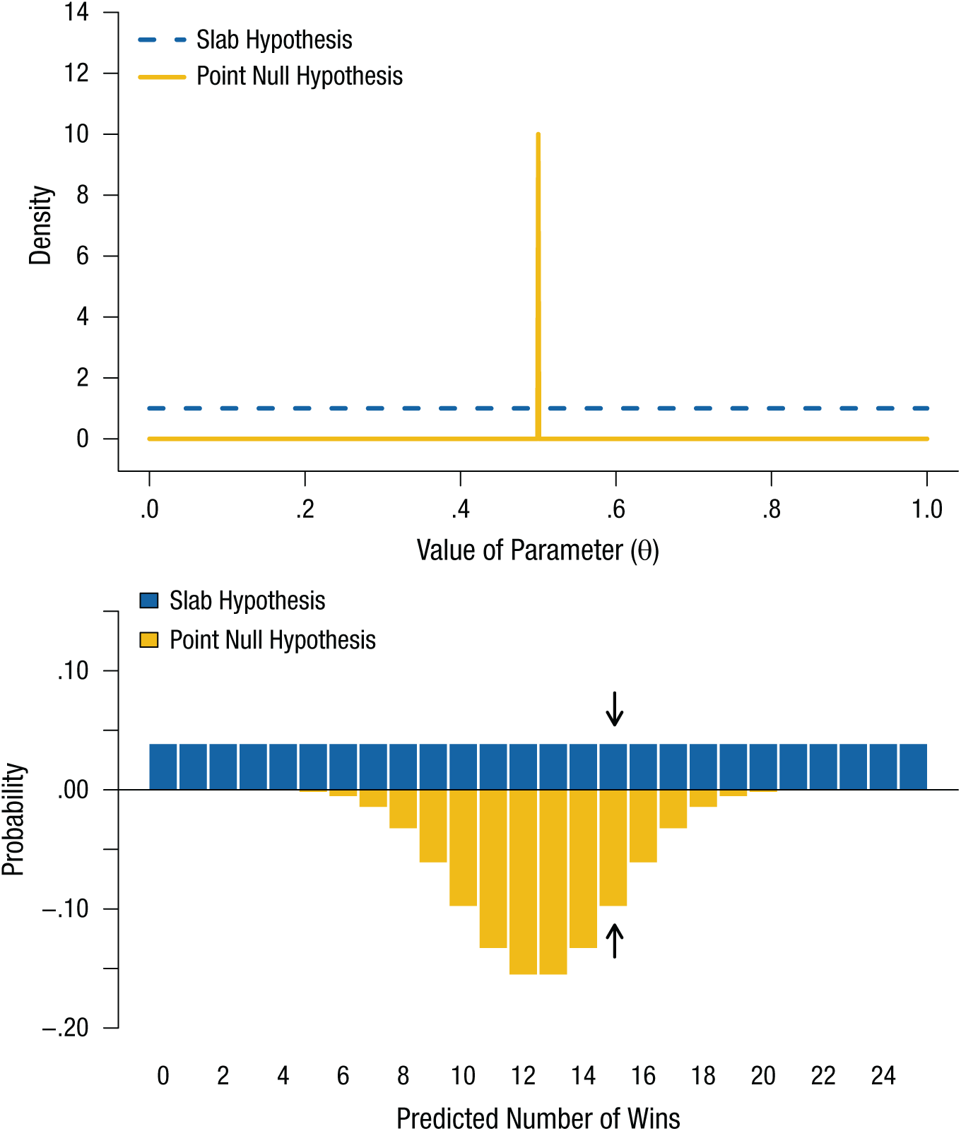
Illustration of point null and slab hypotheses regarding the existence of extrasensory perception, as applied to betting at roulette. The probability densities of the two hypotheses are shown in the top panel. The point null hypothesis is represented by a spike at accuracy of .5, and the slab hypothesis is represented by a horizontal line denoting equal probabilities for all levels of accuracy. The predictions of the two hypotheses are shown in the bottom panel; the Bayes factor is the ratio of the heights of the two bars for a given number of wins. Note that the predictions of the slab hypothesis are similar to those of the nonnegligible-effect hypothesis (shown in the bottom panel of Fig. 4). The arrows highlight the predicted probabilities of 15 successes out of 25 attempts. Like the nonnegligible-effect hypothesis, the slab hypothesis spreads its predictions thinly over the possible range of outcomes, and consequently has lower support than the point null hypothesis given these data.

Two directional hypotheses

Whereas most of the previous comparisons have been for tests of existence, sometimes a researcher is willing to assume the existence of an effect and is interested merely in its direction. This does not seem a desirable approach to investigating ESP, but there are numerous contexts in which such a test might be of interest; for example, a researcher might want to test for a handedness bias or a response bias.

Figure 6 illustrates a comparison of two directional hypotheses. Note that because these hypotheses are clearly separated in the parameter space (top panel), their predictions (bottom panel) are quite different as well. Consequently, comparing directional hypotheses will typically yield stronger discriminative evidence than comparing an existence hypothesis with a nonexistence hypothesis. However, it is important to keep in mind that a comparison between directional hypotheses does not involve any actual null hypothesis—in this example, both the uniformly negative hypothesis and the uniformly positive hypothesis assume the existence of some effect. Consider the case of 15 wins in 25 bets (highlighted by the arrows in Fig. 6). Given such observed data, it would be tempting to compare the two hypotheses and conclude that, because the uniformly positive hypothesis has gained much support, there is evidence for a positive effect and therefore evidence for an effect. But this would be patently wrong—the directional test provides evidence only for a positive effect over a negative effect, assuming there is some effect.² Note especially that this analysis gives zero prior probability to a null effect—in other words, the analysis assumes some effect and could not lead to a conclusion of no effect. One resolution to this problem is discussed in Box 2.

Fig. 6.

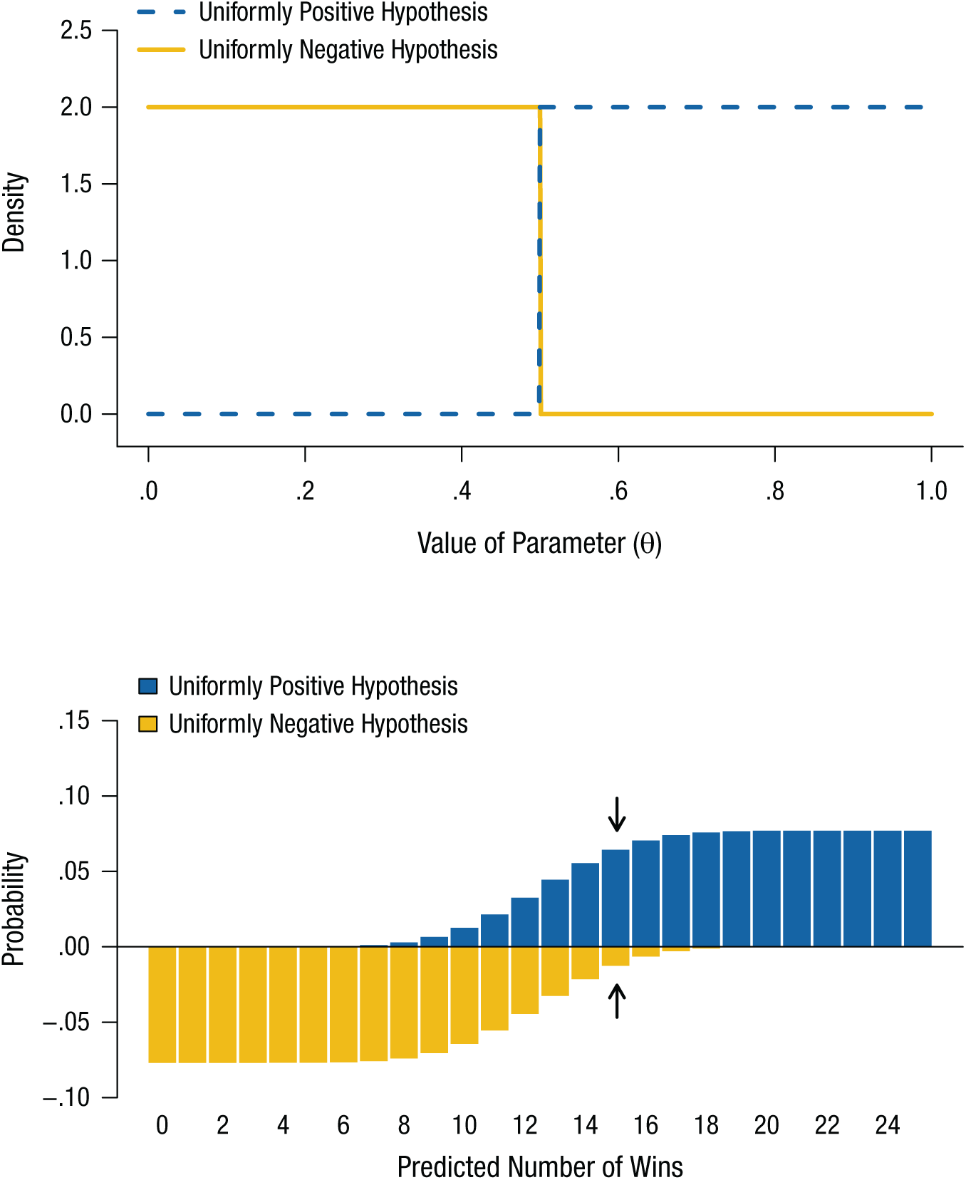
Illustration of uniformly negative and uniformly positive hypotheses regarding the existence of extrasensory perception, as applied to betting at roulette. The probability densities of the two hypotheses are shown in the top panel. The uniformly negative hypothesis is represented by a function with uniformly high probability density in the left half of the interval and 0 density in the right half, and the uniformly positive hypothesis is represented by a function with uniformly high probability density in the right half of the interval and 0 density in the left half. The predictions of the two hypotheses are shown in the bottom panel; the Bayes factor is the ratio of the heights of the two bars for a given number of wins. Note that the predictions of the two hypotheses look quite different and therefore allow for faster accumulation of evidence than do any of the other comparisons of hypotheses in the preceding figures. The arrows highlight the predicted probabilities of 15 successes out of 25 attempts.

Box 2.

Evaluating More Than Two Hypotheses at Once

Not all inference is binary. There are many scenarios under which more than two hypotheses are pitted against one another. We have hinted at one useful example in the main text: One might want to compare two directional hypotheses, a uniformly positive hypothesis (H₊) and a uniformly negative hypothesis (H_–), and a point null hypothesis (H₀), all at once. Nothing prevents researchers from doing this—except perhaps for the fact that they are not accustomed to thinking of evidence for one model over two or more others, and this concept is perhaps somewhat more difficult to communicate than binary comparisons are. Although one can logically and formally work with concepts such as “the odds of H₀:(H₊ ∨ H_–)” (where ∨ means “or” and the colon indicates the odds notation), this is cognitively taxing and a seemingly poor way to communicate.

On the other hand, researchers are quite comfortable talking about probabilities as measures of plausibility. One can use the same predictive probabilities as in Equation 1 to reallocate plausibility across three or more hypotheses. In the case of K hypotheses H₁, H₂, . . . , H_K, the posterior probability of one of them, say H₁, would traditionally be computed with Bayes theorem as follows:

P (H_{1} | D) = \frac{P (H_{1}) P (D | H_{1})}{P (D)},

where D is the observed data and the denominator can be rewritten as

P(D) = P(H₁)P(D | H₁) + P(H₂)P(D | H₂) + . . . + P(H_K)P(D | H_K).

Dividing the numerator and denominator of the right-hand side of Bayes theorem by P(D | H₁), the probability of the data given hypothesis H₁ (known as the likelihood; see Etz, 2018) yields the following useful reformulation of Bayes theorem:

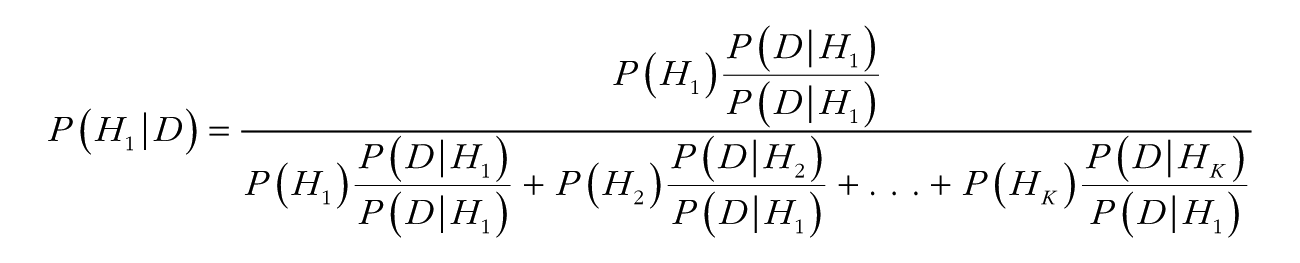
\begin{matrix} P (H_{1} | D) = \frac{P (H_{1}) \frac{P (D | H_{1})}{P (D | H_{1})}}{P (H_{1}) \frac{P (D | H_{1})}{P (D | H_{1})} + P (H_{2}) \frac{P (D | H_{2})}{P (D | H_{1})} + . . . + P (H_{K}) \frac{P (D | H_{K})}{P (D | H_{1})}} \end{matrix}

= \frac{P (H_{1})}{P (H_{1}) + P (H_{2}) B_{2 : 1} + . . . + P (H_{K}) B_{K : 1}},

where B_j_:i is the Bayes factor of hypothesis j over hypothesis i. Using this formula, one can combine the Bayes factors with prior probabilities to obtain posterior probabilities of all the hypotheses in a set of any size.

For example, suppose that in our ESP experiment, we observe 15 wins in 25 attempts (i.e., k = 15 and n = 25), and we want to consider H₀, H₊, and H_–. As shown in Box 1 (Table 1), P(k | H₀) = .0974, P(k | H_–) = .0126, and P(k | H₊) = .0643. We then take the ratios of these probabilities to obtain the following Bayes factors: B_0:– = 7.73, B_0:+ = 1.51, and B_+:– = 5.10. If we say that P(H₀) = .50, P(H₊) = .25, and P(H_–) = .25, then we can combine these with the Bayes factors to obtain the following: P(H₀ | D) = .717, P(H₊ | D) = .237, and P(H_– | D) = .046. Now we are able to make simultaneous statements about the probabilities of some effect (.283) and its direction: If the effect exists, the probability that it is positive is .837 (.237/(.237 + .046)).

Other pairwise comparisons

Hypothesis testing is not limited to comparing two particular values (e.g., .50 vs. .60). As in many of the examples we have presented, researchers can test hypotheses that are statements about ranges of parameters (e.g., θ is greater than .5 or in some small region).

Because the value of θ is not exactly given in such models (in statistics, such a free parameter is sometimes called a nuisance parameter), outside of the simplest cases they cannot be analyzed with classical statistical methods, and a Bayesian approach is required. Fortunately, in the Bayesian framework, these models can be dealt with in the same way as any others: All inferential steps are canonical applications of the calculus of probability.

Of course, our short list of possible null and alternative hypotheses is not exhaustive; the only limit to the possible comparisons is the imagination of the analyst, whose primary concern should be to match the statistical hypotheses as well as possible to the substantive question at hand. For example, a possibility we have not discussed is the interval-and-slab comparison (of which the spike-and-slab comparison is an extreme case). Interval-and-slab comparisons will usually give results similar to those of spike-and-slab comparisons, as long as the null interval is relatively narrow compared with the precision afforded by the data—another instance of the teapot problem (see Berger & Delampady, 1987). Another feature of Bayes factors that we have not discussed in detail is that the Bayes factor between two models can be derived from other pairwise Bayes factors (see Box 3).

Box 3.

Transitivity of the Bayes Factor

The Bayes factor has a convenient property known as transitivity: For hypotheses H₁, H₂, and H₃, if we have the Bayes factor between H₁ and H₂,

B_{1 : 2} = \frac{P (data | H_{1})}{P (data | H_{2})},

and the Bayes factor between H₂ and H₃,

B_{2 : 3} = \frac{P (data | H_{2})}{P (data | H_{3})},

then the product of B_1:2 and B_2:3 gives us the following:

B_{1 : 2} \times B_{2 : 3} = \frac{P (data | H_{1})}{P (data | H_{2})} \times \frac{P (data | H_{2})}{P (data | H_{3})}

= \frac{P (data | H_{1})}{P (data | H_{3})}

= B_{1 : 3} .

That is, the Bayes factor between hypothesis i and hypothesis j can be obtained from their respective pairwise Bayes factors with a common comparison hypothesis k. This property is often useful when multiple models are compared with one reference model, such as in the case of Bayesian analysis of variance (Rouder, Morey, Speckman, & Province, 2012).

Summary

We have focused on one oddly neglected aspect of hypothesis testing: the hypotheses themselves. It is important to keep in mind that although statistical models are always only surrogates for scientific theories, they are the models actually being tested, and it is critical that the statistical models researchers use accurately capture their substantive theories about the data at hand (see also Rouder, Haaf, & Aust, 2018; Vanpaemel, 2010).

Our examples illustrate that different research questions translate into different formal models, and that the evidence for or against an effect can differ depending on precisely what is meant by “no effect.” However, once this translation from a creative scientific theory to a bespoke statistical model is done, the Bayesian machinery turns, and an answer rolls out: One can evaluate the predictive ability of any well-formulated model, and hypotheses that predict the observed data gain plausibility, whereas hypotheses that do not predict the observed data lose it. The Bayes factor acts as an automatic Occam’s razor, penalizing vague hypotheses and rewarding precise predictions. If the observed data are more consistent with the chosen particularization of “null effect” than with the chosen particularization of “some effect,” then the researcher’s belief in the null grows rationally.

R code and the Build-A-Bayes App

Accompanying this article is an online demonstration, available via https://osf.io/mvp53/. In this app, users can choose from a selection of pairwise comparisons and change the data and additional model specifications. This demonstration allows users to interactively experience the effects of changes in model specification, which can be large (e.g., when a directional test, rather than a spike-and-slab comparison, is used) or surprisingly small (e.g., when a point null hypothesis is used instead of a null hypothesis specifying a narrow region of negligible effect). Additionally, Rouder (2017) has provided a similar demonstration in a blog post titled “Roll Your Own: How to Compute Bayes Factors for Your Priors.” This blog post provides R code to compute Bayes factor in a one-sample design.

Discussion and Recommendations

Scientists are tasked with the difficult job of formulating the appropriate scientific question for their context and needs. Once this job is complete, and the scientific question has been translated into an appropriate statistical model, Bayesian methods make it possible to compute the evidence for or against a potential claim.

Two steps in this procedure are especially challenging. The first is the mapping of a substantive question to a formal model (Lee, 2018; Lee & Vanpaemel, 2018; Lee & Wagenmakers, 2013; Matzke, Boehm, & Vandekerckhove, 2018). This requires expertise, judgment, and a measure of artfulness. The second is the computation of the Bayes factor itself. For many common cases (e.g., t tests, analysis of variance, regression), researchers are now building and publishing easy-to-use software (e.g., jasp-stats.org—Wagenmakers, Love, et al., 2018; Wagenmakers, Marsman, et al., 2018; BayesFactor—Morey & Rouder, 2015). However, it will never be the case that all scientific questions will be well addressed by a small set of predefined models. To account for this, other researchers are producing more generic tools and tutorials (Gronau et al., 2017; Matzke et al., 2018; van Ravenzwaaij, Cassey, & Brown, 2018).

The meteoric rise of Bayesian methods in the social sciences is heartening. The recent crisis of confidence in psychology has amplified calls for more powerful and flexible methods—including those with the ability to provide evidence for the nonexistence of an effect—and Bayesian inference is ideally suited for this challenge. But flexibility and power come at a price: The more flexible a tool is, the more extensive its user guide must be. With Bayesian methods, researchers can test any hypothesis they can specify sufficiently. However, each test carries with it potentially unique implementation (i.e., computational) challenges. In this article, we have illustrated methods for testing the null hypothesis for the simplest possible type of data (binary choice). However, these methods are universal—they apply to all sets of hypotheses and models that are sufficiently quantified to make predictions about the data.

The implementation of useful tests and interesting models remains an active field of research and development (e.g., Haaf & Rouder, 2017; Oravecz & Muth, 2018). The main challenge in this endeavor is specifying models that accurately capture theoretical positions. It is incumbent on researchers to specify such models, justify them, and understand how much their particular specification affects the conclusions that can be drawn. These activities are, in our opinion, how analysts add value in uncovering the structure in data (Rouder et al., 2016). Model specification is a creative, nuanced, intellectual activity that relies on scientists’ substantive expertise. We believe that the field of psychology is up to this challenge.

Footnotes

Action Editor

Daniel J. Simons served as action editor for this article.

Author Contributions

All the authors contributed to writing this manuscript.

Declaration of Conflicting Interests

The author(s) declared that there were no conflicts of interest with respect to the authorship or the publication of this article.

Funding

The authors were supported by National Science Foundation Grant 1534472 to J. Vandekerckhove and by National Science Foundation Graduate Research Fellowship Program Grant DGE-1321846 to A. Etz.

Prior Versions

A prior version of this article is available at .

Notes

References

Bayes

(1763). An essay towards solving a problem in the doctrine of chances. By the late Rev. Mr. Bayes, F. R. S. Communicated by Mr. Price, in a letter to John Canton, A. M. F. R. S. Philosophical Transactions of the Royal Society, 53, 370–418.

Bem

D. J.

(2011). Feeling the future: Experimental evidence for anomalous retroactive influences on cognition and affect. Journal of Personality and Social Psychology, 100, 407–425.

Berger

J. O.

Delampady

(1987). Testing precise hypotheses. Statistical Science, 2, 317–352.

Cox

R. T.

(1946). Probability, frequency and reasonable expectation. American Journal of Physics, 14, 1–13.

de Finetti

(1974). Theory of probability (Vol. 1). New York, NY: John Wiley & Sons.

Edwards

Lindman

Savage

L. J.

(1963). Bayesian statistical inference for psychological research. Psychological Review, 70, 193–242.

Etz

(2018). Introduction to the concept of likelihood and its applications. Advances in Methods and Practices in Psychological Science, 1, 60–69.

Etz

Vandekerckhove

(2018). Introduction to Bayesian inference for psychology. Psychonomic Bulletin & Review, 25, 5–34.

Gronau

Q. F.

Sarafoglou

Matzke

Boehm

Marsman

. . . Steingroever

(2017). A tutorial on bridge sampling. Journal of Mathematical Psychology, 81, 80–97.

10.

Haaf

J. M.

Rouder

J. N.

(2017). Developing constraint in Bayesian mixed models. Psychological Methods, 22, 779–798.

11.

Jaynes

E. T.

(2003). Probability theory: The logic of science. Cambridge, England: Cambridge University Press.

12.

Jeffreys

(1939). Theory of probability (1st ed.). Oxford, England: Oxford University Press.

13.

Jeffreys

(1961). Theory of probability (3rd ed.). Oxford, England: Oxford University Press.

14.

Kass

R. E.

Raftery

A. E.

(1995). Bayes factors. Journal of the American Statistical Association, 90, 773–795.

15.

Laplace

P.-S.

(1829). Essai philosophique sur les probabilités [Philosophical essay on probabilities]. Brussels, Belgium: H. Remy.

16.

Lee

M. D.

(2018). Bayesian methods in cognitive modeling. In Wixted

(Ed.), Stevens’ handbook of experimental psychology and cognitive neuroscience (4th ed., pp. 37–84). Hoboken, NJ: Wiley.

17.

Lee

M. D.

Vanpaemel

(2018). Determining informative priors for cognitive models. Psychonomic Bulletin & Review, 25, 114–127.

18.

Lee

M. D.

Wagenmakers

E.-J.

(2013). Bayesian cognitive modeling: A practical course. Cambridge, England: Cambridge University Press.

19.

Matzke

Boehm

Vandekerckhove

(2018). Bayesian inference for psychology, part III: Parameter estimation in nonstandard models. Psychonomic Bulletin & Review, 25, 77–101.

20.

Mitchell

T. J.

Beauchamp

J. J.

(1988). Bayesian variable selection in linear regression. Journal of the American Statistical Association, 83, 1023–1032.

21.

Morey

R. D.

Rouder

J. N.

(2011). Bayes factor approaches for testing interval null hypotheses. Psychological Methods, 16, 406–419.

22.

Morey

R. D.

Rouder

J. N.

(2015). BayesFactor: Computation of Bayes factors for common designs (R package Version 0.9.12-2) [Computer software]. Retrieved from https://cran.r-project.org/web/packages/BayesFactor/

23.

Myung

I.-J.

Pitt

M. A.

(1997). Applying Occam’s razor in modeling cognition: A Bayesian approach. Psychonomic Bulletin & Review, 4, 79–95.

24.

Oravecz

Muth

(2018). Fitting growth curve models in the Bayesian framework. Psychonomic Bulletin & Review, 25, 235–255.

25.

Rogers

J. L.

Howard

K. I.

Vessey

J. T.

(1993). Using significance tests to evaluate the equivalence between two experimental groups. Psychological Bulletin, 113, 553–565.

26.

Rosenkrantz

R. D.

(Ed.). (1983). E. T. Jaynes: Papers on probability, statistics and statistical physics (Synthese Library, Vol. 158). Boston, MA: Kluwer Academic.

27.

Rouder

J. N.

(2017). Roll your own: How to compute Bayes factors for your priors [Web log post]. Retrieved from https://psyarxiv.com/nvsm5

28.

Rouder

J. N.

Haaf

J. M.

Aust

(2018). From theories to models to predictions: A Bayesian model comparison approach. Communication Monographs, 85, 41–56.

29.

Rouder

J. N.

Haaf

J. M.

Vandekerckhove

(2018). Bayesian inference for psychology, part IV: Parameter estimation and Bayes factors. Psychonomic Bulletin & Review, 25, 102–113.

30.

Rouder

J. N.

Morey

R. D.

(2017). Teaching Bayes’ theorem: Strength of evidence as predictive accuracy. The American Statistician. Advance online publication. doi:10.1080/00031305.2017.1341334

31.

Rouder

J. N.

Morey

R. D.

Province

J. M.

(2013). A Bayes factor meta-analysis of recent extrasensory perception experiments: Comment on Storm, Tressoldi, and Di Risio (2010). Psychological Bulletin, 139, 241–247.

32.

Rouder

J. N.

Morey

R. D.

Speckman

P. L.

Province

J. M.

(2012). Default Bayes factors for ANOVA designs. Journal of Mathematical Psychology, 56, 356–374.

33.

Rouder

J. N.

Morey

R. D.

Wagenmakers

E.-J.

(2016). The interplay between subjectivity, statistical practice, and psychological science. Collabra: Psychology, 2, Article 6. doi:10.1525/collabra.28

34.

Russell

(1957). Why I am not a Christian and other essays on religion and related subjects. New York, NY: Simon & Schuster.

35.

Savage

L. J.

(1951). The theory of statistical decision. Journal of the American Statistical Association, 46, 55–67.

36.

Vandekerckhove

Matzke

Wagenmakers

E.-J.

(2015). Model comparison and the principle of parsimony. In Busemeyer

Townsend

Wang

Z. J.

Eidels

(Eds.), Oxford handbook of computational and mathematical psychology (pp. 300–319). Oxford, England: Oxford University Press.

37.

Vanpaemel

(2010). Prior sensitivity in theory testing: An apologia for the Bayes factor. Journal of Mathematical Psychology, 54, 491–498.

38.

van Ravenzwaaij

Cassey

Brown

S. D.

(2018). A simple introduction to Markov Chain Monte–Carlo sampling. Psychonomic Bulletin & Review, 25, 143–154.

39.

Wagenmakers

E.-J.

Love

Marsman

Jamil

Verhagen

. . . Morey

R. D.

(2018). Bayesian inference for psychology. Part II: Example applications with JASP. Psychonomic Bulletin & Review, 25, 58–76.

40.

Wagenmakers

E.-J.

Marsman

Jamil

Verhagen

Love

. . . Morey

R. D.

(2018). Bayesian inference for psychology. Part I: Theoretical advantages and practical ramifications. Psychonomic Bulletin & Review, 25, 35–57.

41.

Wrinch

Jeffreys

(1921). On certain fundamental principles of scientific inquiry. Philosophical Magazine, 42, 369–390.

Bayesian Inference and Testing Any Hypothesis You Can Specify

Abstract

Keywords

Occam’s Razor and Russell’s Teapot

Jeffreys’s Platitude

Statistical Inference

Possible Scenarios

The point null hypothesis

The uniformly positive hypothesis

The Bayes Factor

Other Possible Scenarios

The competing-point hypothesis

The positive-decay hypothesis

The negligible-effect hypothesis

The spike-and-slab comparison

Two directional hypotheses

Other pairwise comparisons

Summary

R code and the Build-A-Bayes App

Discussion and Recommendations

Footnotes

Action Editor

Author Contributions

Declaration of Conflicting Interests

Funding

Prior Versions

Notes

References