Database-Centric Method for Automated High-Throughput Deconvolution and Analysis of Kinetic Antibody Screening Data

Abstract

The state-of-the-art industrial drug discovery approach is the empirical interrogation of a library of drug candidates against a target molecule. The advantage of high-throughput kinetic measurements over equilibrium assessments is the ability to measure each of the kinetic components of binding affinity. Although high-throughput capabilities have improved with advances in instrument hardware, three bottlenecks in data processing remain: (1) intrinsic molecular properties that lead to poor biophysical quality in vitro are not accounted for in commercially available analysis models, (2) processing data through a user interface is time-consuming and not amenable to parallelized data collection, and (3) a commercial solution that includes historical kinetic data in the analysis of kinetic competition data does not exist. Herein, we describe a generally applicable method for the automated analysis, storage, and retrieval of kinetic binding data. This analysis can deconvolve poor quality data on-the-fly and store and organize historical data in a queryable format for use in future analyses. Such database-centric strategies afford greater insight into the molecular mechanisms of kinetic competition, allowing for the rapid identification of allosteric effectors and the presentation of kinetic competition data in absolute terms of percent bound to antigen on the biosensor.

Introduction

Monoclonal antibodies (mAbs) represent the largest class of recombinant protein therapeutics within the biopharmaceutical industry. In most high-throughput discovery applications, the directed evolution of mAb-based molecules is conducted using a large library of sequences, on the order of 10¹⁰ molecules, ¹ against a single antigen. After conducting preliminary screening, rounds of affinity maturation (AffMat) are often used to identify the sequence mutations that will improve the affinity of the parental interaction. ² Typically, surface plasmon resonance (SPR) or biolayer interferometry (BLI) instruments are used to measure these in vitro affinities. Both technologies acquire data in real time using a functionalized sensor surface. Exposure of a functionalized sensor to a protein of interest permits capturing the protein to the surface (loading step). The affixed protein is then exposed to a solution containing the binding partner (association step), followed by exposure of the sensor to analyte-free buffer to permit the complex to dissociate (dissociation step). Currently, continuous-flow SPR technology is the industry gold standard for kinetic characterization of mAb-antigen interactions. However, this technology’s limited throughput and lack of flexibility reduce its utility as a high-throughput screening (HTS) technology. For instance, GE Health Science’s (Marlborough, MA) Biacore 8k SPR system can record a maximum of eight reactions per acquisition cycle, whereas the alternative static sample BLI technology can record a maximum of 96 reactions per acquisition cycle using Pall ForteBio’s (Melano Park, CA) Octet HTX instrument. Improvements in throughput of SPR-based instruments have been addressed recently with advances in the development of next-generation SPR imaging (SPRi) instruments. SPRi technology, in the case of Wasatch Microfluidics’ (Salt Lake City, UT) MX96 SPRi instrument, uses microfluidic printing to produce arrays of spotted samples that permit the equivalent throughput of the Octet HTX with a maximum of 96 reactions per acquisition. Although the throughput of both technologies is converging, there remain considerable differences between the two technologies. BLI technology is quantitatively less accurate for measurements of slow dissociation rates ³ and very fast association rates, ⁴ and it is generally less sensitive than SPR-based instrumentation. However, when considering the trade-off of quantitative accuracy for throughput, BLI technology is positioned well for early discovery screening applications. One notable advantage that BLI has over SPR is the minimal experimental preparation and tuning required to interrogate hundreds of samples en masse. Another advantage is the flexibility to operate with any sensor format, ranging from a single sensor to 96 sensors per single acquisition. BLI sensors can also be functionalized, loaded, and blocked offline to maximize the duty cycle of the instrument. In addition, due to BLI being less sensitive to the refractive index of bulk media than SPR-based instruments, sensor consumption can be minimized by eliminating or reducing the number of dedicated reference sensors. Previous work has also demonstrated that the Octet HTX has the additional advantage of being capable of high-throughput loading of material suspended in crude culture supernatant, which further increases the screening throughput by eliminating upstream sample purification steps. ⁵

For typical experiments using the Octet HTX, an investigator loads either an antibody or antigen to the BLI sensor, exposes the sensor to a potential binder of interest, and subsequently exposes the complex to analyte-free buffer to permit dissociation of the complex. Data are collected in real time and subsequently analyzed by fitting analytical models to the raw responses. Successful identification of the appropriate binding equations for each interaction permits the parameterization of the association rates (k_a), dissociation rates (k_d), equilibrium dissociation constant (K_D), and associated amplitudes. For AffMat experiments, these data are used to identify, rank, and filter the mAb clones that have become more desirable than the parental sequence. The Octet HTX instrument can also perform kinetic competition assays to kinetically determine epitope diversity (i.e., binning). In this format, an investigator would repeat the previous kinetic experiment except for the last step where, instead of exposing the complex to analyte-free buffer, the mAb-antigen complex is exposed to a comparison molecule, either an antibody or ligand to the antigen. If this secondary binding event produces a positive amplitude, it is considered to likely bind a different epitope than the primary binder and is therefore in a different epitope bin and considered a noncompetitor. Likewise, if no significant positive amplitude is observed, the secondary antibody would presumably compete for the same epitope bin and would be considered competitors. ⁶

Current commercial software solutions for identifying epitopic kinetic competition generally use a single-amplitude cutoff threshold that is likely not to be appropriate for acquisitions containing proteins ranging in molecular weights. The masses of the molecules being investigated have a direct effect on the maximum achievable amplitude when using either SPR or BLI technologies and should therefore be accounted for in the analysis of the data. Employing a single cutoff threshold requires the experiment to be designed with consideration of the analysis procedure and has the additional disadvantage of ignoring negative amplitudes that could be indicative of allosteric kinetic competition.

Although identification of allostery is not novel, the field currently lacks commercial software tools for the high-throughput identification of such effectors. Allostery is a phenomenon of energetic coupling between two nonoverlapping binding sites that is propagated by changes in local or gross (i.e., conformational) dynamic modes that are induced by a noncovalent interaction at one or more binding sites.^7,8 The combination of kinetic binding and kinetic competition data enables an investigator to identify this energetic coupling in the form of both positive (increase of affinity) and negative (decrease of affinity) allosteric effectors based on differences of the binding kinetics in the presence and absence of an effector molecule. Recent work from Wasatch Microfluidics recently proposed an alternative displacement phenomenon that is similarly observed with its analysis. Using the MX96 SPRi instrument, Abdiche et al. ⁹ were able to conduct high-density binning experiments and identify kinetic competitors that have overlapping epitopes and thus potentially operate via a mechanism not entirely consistent with allostery. This work demonstrates the need for software improvements in the field that can provide improved analytical insight and solutions for the rapid analysis of large volumes of correlated data.

Manufacturer-supplied data analysis software for kinetic binding and competition data currently does not address two outstanding considerations of typical data. First, nonspecific binding can be an issue when screening impure samples or when the biophysical properties of the molecules being surveyed are not optimal ex vivo. Some targets will tend to form soluble and insoluble aggregates, which can lead to nonspecific binding to the sensor or aggregation facilitated by the high local concentration of protein at the sensor surface. Similarly, mAbs surveyed early in the discovery process may have poor biophysical properties since selective pressure and rational engineering to eliminate nonspecific binding often takes place postdiscovery. In instances where using these suboptimal conditions is unavoidable, the observed binding curves are typically multiphasic with both fast and slow association and dissociation components convolved in the observed raw signal. The challenge for analyzing suboptimal data such as these is modeling the nonspecific response component without extending the acquisition times to permit an accurate exponential fit of the slow phase and without running secondary experiments.

Another poorly addressed data analysis consideration involves the assignment of epitopic or allosteric competitors in the absence of the individual binding kinetics and molecular weights (MW) of the comparison molecules. Ideally, the k_d of the primary antibody-antigen pair would have no appreciable decay over the experimental window, but this requirement precludes early screening of bin diversity. Since this is rarely the case during early discovery experiments, consideration of the primary complex’s dissociation rate must be factored in to accurately assign bins. Furthermore, if the antigen and the comparison molecule are of significantly different MW, then the raw binning response will not be scaled appropriately, making the cutoff determination sensitive to the individual pairings.

To address the above concerns, it is of primary importance to first optimize the experimental conditions to reduce heterogeneous binding artifacts as much as possible by adjusting ligand surface density, association and dissociation times, analyte concentrations, and buffer conditions, as well as ensuring all reagents are homogeneous. Quantitative accuracy will always depend on data quality, regardless of the analysis being performed. However, under HTS conditions, compromises between data quality and duty cycle are necessary to strike a suitable balance between efficiency and information content. This ultimately requires that a single set of experimental conditions be applied indiscriminately to all samples, which necessitates that additional experiments on lead molecules be performed downstream to obtain the quantitative accuracy required for thorough characterization of the developed molecules. Herein we describe a method for processing parallelly acquired data from multiple high-throughput instruments using a database-centric method for end-to-end automated analysis. This method only requires users to configure the instrument with the experimental parameters and then start the experiment. Postprocessed data are presented with simple and targeted visualizations and descriptive comments for rapid human validation. Implementation of this automation strategy using forty 96-well plate experiments saves over 9 h of human data processing and analysis time compared to manual analysis using the manufacturer-supplied software. This method also provides expanded and more consistent data interpretation, as well as queryable managed data.

Materials and Methods

Biological Materials

All mAb samples were produced, purified, and validated in-house using Adimab’s proprietary yeast platform. Antigens were purchased from various vendors. Experiments were conducted with either protein A purified immunoglobulin G (IgG) in Phosphate Buffered Saline (PBSF), 0.1% Bovine Serum Albumin or culture supernatant. Fab domains were produced by treating intact IgG samples with Papain. BLI sensors were purchased from ForteBio and regenerated up to 10 times. ⁵

Instrument Configuration

Two ForteBio Octet HTX instruments were used in 96-channel mode with Anti-Mouse IgG Fc Capture (AHC), streptavidin (SA), or Anti-Human IgG Quantitation (AHQ) sensors. Sensors were functionalized with a loading step by dipping the sensors into 100 nM solution of the protein of interest until the acquisition signal reached a 0.8 nm threshold. If required, sensors were blocked offline with the appropriate blocking reagent for 5 min and washed for 30 min in analyte-free buffer. Instrumentation was driven by manufacturer-supplied software (versions 8.2 and 9.0). Sample names and concentrations were input into the plate data page, and sensor-associated proteins were identified in the “information” column on the sensor data page. Kinetic experiments were collected with either a 90 or 180 s baseline, a 180 s association phase, and a 180 s dissociation phase. Binning experiments were collected in five steps: 90 s of baseline 1, 90 s of a sensor binding check with the secondary binder, 90 s of baseline 2, 180 s of association, and 180 s of dissociation in the well containing the secondary mAb. All files were saved into a shared network drive with a naming convention that identifies the format of the experiment.

Database Configuration

Adimab’s Atlas product comprises a PostgresSQL (https://www.postgresql.org/) relational database (version 9.4) and a software application layer developed at Adimab, which consists of both a Microsoft C# ASP.NET component (Micorsoft, Redmond, WA) and Python Django (https://www.djangoproject.com/) framework component. The software application provides a web-based user interface for viewing and interacting with data as well as an application program interface (API) for uploading, downloading, and querying experiment data over the network via HTTP. The API was designed to allow external programs to work with the experiment data in a common nonproprietary machine-readable format, JSON, or as spreadsheets. The queryable experimental data stored in Atlas include kinetics (response curves and fits), molecular masses, and protein sequences.

Automation Configuration

An in-house software tool was installed on a server to watch the shared network drive where data are collected. Upon completion of data collection, processing is initiated using a trigger file. Manipulations of the data are contributed to and depend on the use of the fortebiopkg python package (https://github.com/bostonautolytics/fortebiopkg). During processing of the collected data, any required information from previous experiments that had been stored in the Atlas database is programmatically queried via the Atlas API using unique sample IDs shared across experiments.

With binning data, the automation tool exports an Excel file containing image representations of the data, analysis calls, flags, experimental parameters, and specific comments for each sensor. After manual review of this Excel file, to ensure that the automated calls are consistent with the generated plots, it is uploaded along with the raw data via the Atlas web interface into the Atlas database for future retrieval. In the case of kinetic binding data, the automation tool programmatically uploads the results directly using the Atlas API, where it can be visually reviewed and confirmed in an interactive Atlas web interface, modified if necessary before being finalized, and stored in the Atlas database for future retrieval. In both cases, the manual review generally takes less than 10 min for 96 samples as the automated calls are consistent with human interpretation in approximately 90% of cases. Human interpretation is required in cases where the binning call is ambiguous and additional data need to be considered, as well as to ensure that the generated fits of the kinetic data produce reasonable parameters and have acceptable residuals.

Self-Sensor Baseline Correction

Depending on how long sensors are equilibrated prior to runtime, linear or nonlinear baseline drift may be observed. Manufacturer-supplied software does not provide an option to subtract baseline measurements made with the same sensor, although it does provide reference subtraction options that require the use of additional sensors. However, the use of additional sensors for reference measurements does not account for sensor-to-sensor, channel-to-channel, or well-to-well variability that may lead to sensor-specific drift. To reduce sensor consumption and apply self-sensor corrections, a collection of at least 90 s of baseline data with the loaded sensor is used for self-sensor correction. Baseline data will show no drift, a linear response, or an exponential equilibration phase. The range of modes that can be observed in baseline data renders the automated correction of variable baseline responses challenging, especially when differentiating between a linear and exponential phase over short collection times. ¹⁰ To best accommodate all possible scenarios, only the last third of the baseline data is fit to a linear model and subtracted from the entire run. After subtraction, the physical limits of the experiment are verified and the data are recorrected, if required, by fitting the last 10% of the association data to a linear model. If the slope of the association data is less than 0, the entire data series is corrected to a slope of 0. If the resulting correction produces a positive slope in the association data, no baseline correction is applied.

Linear Approximation of Slow Phases in Kinetic Data

A 1:1 stoichiometry analytical binding model describing the association phase (equation (1)) and dissociation phase (equation (2)) was used for the basis of the kinetic data analysis of baseline

$$R_{on}=\left(\frac{R_{max}}{1+\frac{k_d}{k_a\cdot C_{pro}}}\right)\left(1-e^{-X\left(k_a\cdot C_{pro}+k_d\right)}\right)$$

$$R_{off}=A_s\cdot (A_{on}-B_{NS})\cdot \left(e^{-k_d\left(X-X_0\right)}\right)+B_{NS}$$

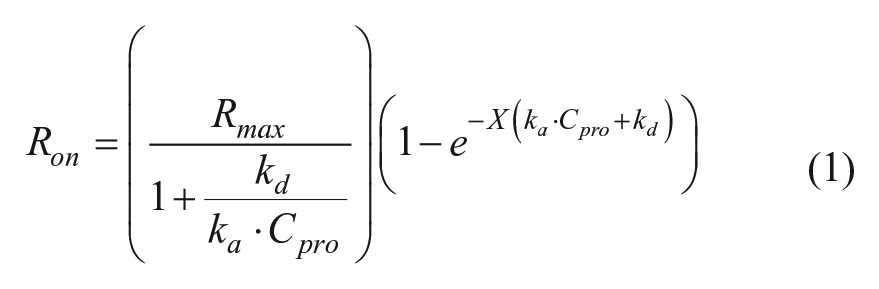
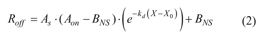
subtracted data, where R_on and R_off are the observed experimental signals of the respective phases, A_s is an arbitrary amplitude scalar that describes the total amplitude (association and dissociation) contribution of the data being ignored by the deconvolution process, A_on is the amplitude of the association phase calculated using equation (1) with X = X₀, R_max is the maximum binding capacity, k_a is the kinetic association constant, k_d is the kinetic dissociation constant, C_pro is the concentration of protein in solution, B_NS is the amplitude contribution of nonspecific binding, and X₀ is the time-zero offset of the dissociation phase. ¹¹ Although A_s and A_on could be combined into a single term, they were kept separate for programmatic convenience due to A_on being dependent on equation (1). In the manufacturer-provided software package, selection of the “1:1 model” uses similar fitting equations where B_NS = 0, but selection of “partial fit” will allow the B_NS term to float. These models work well when B_NS describes irreversible aggregation on the sensor, but in some cases, the nonspecific binding is reversible. In such cases, using either method will result in the model becoming asymptotic through only part of the data at longer times, the exponential phase having poor residuals at early time points, or both. To account for this slow phase, a linear term can be added to the fitting model to approximate the data as long as it is suitably applied (equation (3)).

$$R_{off}=A_s\cdot (A_{on}-c)\cdot \left(e^{-k_d\left(X-X_0\right)}\right)+m\cdot \left(X-X_0\right)+c$$

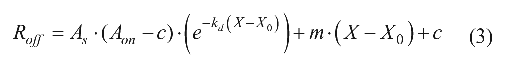
In equation (3), m is the linear slope that is used to approximate the slow exponential response, and c is the sum of the y-intercept of the linear term and B_NS. Equation (3) can only be used in place of equation (2) when the slow phase can realistically be approximated by a linear function, which is when there is no more than ~0.5 lifetimes (τ = k⁻¹) of the slow response in the observed data (equation (4)).

$$M_{co}=-0.01146\cdot e^{\left(\frac{-t}{77.5583}\right)}-0.07192\cdot e^{\left(\frac{-t}{10.3}\right)}$$

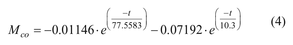
Equation (4) is a look-up formula that describes the relationship of experimental collection time (t) and minimum slope cutoff (M_co) of normalized data. This equation was obtained empirically, by fitting 0.5 τ of data using different experimental window times from 10 to 500 s and varying kinetic rate constants. The result is that m from equation (3) must be ≥ M_co given the experimental collection window, t, for the linear approximation to be valid. In the case that the linear approximation is not valid, a double exponential model can be fit to the dissociation phase by replacing equations (1) and (2) with a 1:2 stoichiometry model. However, such binding events would require additional experiments be performed to accurately differentiate the two dissociation rates. Using a typical dissociation collection time of 180 s, where sensitivity of M_co is maximized, precludes the accurate fitting of a two-state model using the rule of thumb of requiring 95% of the slowest exponential phase (3 τ) be collected to accurately fit a kinetic response having more than one kinetic phase.

Dissociation Model Determination

Equation (2) is first fit to the data with A_on = 1 and B_NS = 0 using a Levenberg-Marquardt optimizer (full fit). If the R² is above 0.95 and the residuals do not exceed 5% of the maximal signal, the model is assumed to be valid. In the case that either of these conditions is not met, equation (2) is fit again with B_NS being allowed to float (partial fit). If the quality conditions are again unmet, equation (3) will be used (decon fit). If the results of fitting the data with equation (3) fail to meet the slope cutoff determined by equation (4), the results of the previous fit will be reported and the sensor will be commented to note the potential multiphasic response.

In cases where the total amplitude change of the dissociation step is less than 20%, the data are treated differently because the lack of signal change indicates poor sample quality with significant nonspecific binding on the sensor or avid binding with insufficient data to accurately fit. In addition, when screening culture supernatant directly, it is possible to observe a fast initial dissociation rate of small amplitude, which is likely nonspecific binding of media-related components. If 15% of the signal change occurs within the first 5 s with a total amplitude change of 20% or less over 180 s, reversible nonspecific binding is assumed to be the cause of the initial signal decay. In this scenario, only data collected after the first 5 s will be considered further using the 5 s point as X₀. The 5% rule^12,13 is applied to the dissociation signal where a 5% decrease in signal at 90 s from X₀ is required to reasonably fit the k_d data. If the 5% rule is met, the data are fit using equation (2) with B_NS = 0 and k_d = –ln(0.95)/t, as has been previously described. ¹² If the 5% rule is not met and the total signal decay is ≤20%, the data will appear linear over the collection window and therefore will not produce a reliable fit with a 180 s acquisition time. In this case, the dissociation rate is estimated as k_d < –ln(0.95)/t for an initial parameter. After fitting, the k_d parameter is compared to the k_d detection limit defined by the 5% rule. If the final k_d parameter exceeds this limit, it will be flagged with a comment by the algorithm. It should be noted that the sensitivity of the Octet instrument operating in the highest throughput mode is much lower than SPR instruments from which the rule was originated. The effect is that some traces may result in erroneous decisions between fitting the data using equation (2) with B_NS = 0 and estimating the dissociation rate as k_d < –ln(0.95)/t. However, the experiments being described occur in nonoptimized sample conditions with a fixed collection time of 180 s. Under these experimental conditions, it is likely that both estimates of these observed slow dissociation rates will be inaccurate, and such samples will require more careful and thorough characterization postdiscovery.

Deconvolution of k_d and k_a with Suboptimal Data Quality

Determination of the dissociation rate model will reveal the deconvolved k_d value after fitting the dissociation phase of the data. Deconvolution of the k_a parameter requires this k_d parameter as well as m and C, if required, to be held constant while globally fitting the sensogram to equations (1) and (2) or equations (1) and (3). If the linear approximation is not required, the data are fit with A_s = 1. The validity of the k_d parameter extracted from the initial fit requires that two assumptions be valid: the dissociation rate is concentration independent, and there is no significant contribution of binding to the sensor. These assumptions will hold true if the dissociation step is performed in dilute buffer. As this is often the case, fixing the value of k_d allows for the solution of the requisite k_a for the dissociation model to be true, given the raw signal of the association phase. This allows for an approximate k_a value to be solved for even when the data are of suboptimal quality, including association phases that saturate the sensor, involve a subpopulation of aggregated species, or contain artifactual binding contributions from performing sensor loading in cell culture supernatant samples. Using this method, the quality of data will obviously have an impact on the quantitative success as the raw signal is assumed to be mostly artifact free and not mass transport limited. Ideal deconvolution would be performed using a known K_D value, but it is unlikely that an investigator would have this information prior to the experiment. Highly convolved association data will produce poor results as the raw signal is still used to constrain the fit of k_a in the absence of a known K_D. For screening purposes under suboptimal conditions, we suggest relying on k_d to rank the resulting data as it is the highest confidence measurement achievable in suboptimal conditions, and it is less susceptible to mass transport artifacts than k_a. The dissociation deconvolution is also less dependent on the raw data, assuming that the dissociation rate of interest is the faster observable rate.

Molecular Weight Correction of Data

SPR data, unlike BLI data, can achieve a quantitative data correction by scaling the amplitude of the response by relative molecular weights of the molecule. The SPR response has previously been shown to be proportional to the refractive index of the sample as well as to the concentration of protein adhered to the sensor.^14,15 It has also been demonstrated that different proteins appear to have nearly identical refractive indices.^15–17 Therefore, the molecular weight of a protein will also scale proportionally with signal amplitude. Thus, scaling of SPR data can reasonably be performed by multiplication of the signal by a scalar, defined by the ratio of molecular weights of the molecules of interest, as this adjusts the amplitude and not the rate constant of the response. Correction of the data is made relative to the MW of the molecule used in the association step in binning experiments.

Using BLI data, only a semiquantitative correction can be achieved as the orientation of the molecules, relative to the light path, can have substantial effects on the measured average thickness of the biolayer. In modeling of experimental solution measurements, proteins are often approximated as solid spheres, which depend on the valid assumption of the molecules being able to freely tumble in 3D space on timescales much faster than the experimental timescale. In direct violation of this assumption is the requirement for molecules to be immobilized on the sensor surface for BLI measurements. Immobilization imposes a significant orientation bias, rendering the typical volumetric relationship invalid. Plotting the unweighted average dimensions of crystal structures of several globular proteins of varying molecular weights (Suppl. Table S1 and Suppl. Fig. S1a) describes the relationship between molecular weight and expected biolayer thickness of a randomly immobilized protein. For molecules having a molecular weight of at least 40 kDa, the relationship can be sufficiently described with either the volumetric model or with a linear approximation using a slope of 2E5 nm·Da⁻¹ and a y-intercept of 3.82 nm. However, the dimensions of a mAb molecule are not approximated well by either model due to its unique Y-shape and the consistent relative location of the binding domains, which impose a significant and consistent orientation bias. Because the complementary determining regions (CDRs) that bind the target molecule are always localized at one end of the molecule, lengthwise, and assuming that it is unlikely that IgG will efficiently bind to the target molecule parallel to the sensor surface due to excluded volume effects, the smallest dimension of the molecule can be de-weighted or removed from the average dimension calculation as there should be a significant orientation bias favoring configurations of the mAb with the longer dimensions approaching parallel angles to the light path. The result is that the same proportionality calculation used for SPR data can be applied to BLI data if the target molecule is a globular protein between approximately 30 and 100 kDa (based on the average dimensional standard deviation) and the secondary binder is either a Fab or mAb molecule (Suppl. Fig. S1a). Experimental results obtained from loading randomly biotinylated antigen to an SA BLI sensor and binding a set of eight Fab molecules or their corresponding mAb molecules of threefold higher MW yield an average scaling factor of 2.51 ± 0.57-fold (Suppl. Table S2 and Suppl. Fig. S1b), consistent with the de-weighted mAb model (Suppl. Fig. S1a). These results suggest that the same scaling procedure applied to SPR data can be reasonably applied to BLI data for semiquantitative results. Notably, these measurements remain sensitive to the orientations of both the primary and secondary binder and, therefore, should only be used for comparisons across data sets of the same molecules throughout screening applications. However, because the scaling is using a linear model instead of an exponential model, the relative amplitude changes within a data set will be uniform, resulting in the valid scaling of kinetic competition data that is collected using molecules with disparate MWs. Such scaling improves the detection of kinetic competitors by reducing ambiguous calls in screening applications. Postdiscovery, SPR experiments will be required for quantitative accuracy.

Kinetic Correction of Binning Data

Binning data are collected in five steps after loading and blocking the sensor with the primary binder. First, 90 s of data is collected in analyte-free media (baseline 1), and then 90 s of data is collected with the sensors dipped into the wells containing the secondary binder (sensor binding check). Even under the best conditions, the secondary binder may have some low levels of nonspecific sensor binding, which is washed off in the third step with a second exposure to analyte-free media for 90 s (baseline 2). The experiment then continues with a 180 s exposure to the analyte of interest (association step) followed by a 180 s exposure to the secondary binder (binning step). Baseline subtraction of baseline 1 is conducted across the entire sensogram. Baseline 2 is then extrapolated to either y = 0 or to the end of the dissociation phase, whichever comes first, and subtracted from itself, the association phase, and the binning phase. The sensor binding check, if it exceeds a signal-to-noise ratio of 3, is fit to a single exponential model and subtracted from the binning response phase. The data are then normalized between 0 and 1 using the first and last points of the association phase such that the data are scaled relative to the amount of antigen on the sensor. Kinetic data are then queried from the database such that the latest acquired data using the same proteins, at the same concentration, on the same sensors, and in the same orientation will be returned. These queried data are likewise normalized between 0 and 1 with respect to the association phase and fit to a single exponential decay. A model of the fit parameters is then subtracted from the signal in the binning response. The corrected binning response approximates what would be observed had the antigen not been able to dissociate from the sensor. Scaling by MW and normalizing the amplitudes result in a scale equivalent to percent bound with respect to available antigen on the sensor, which provides a universal scale that can be used to compare data across data sets and with proteins ranging in size. For SPR data, this scaling is quantitative while BLI data will result in semiquantitative estimates.

Results and Discussion

Dissociation Rate Deconvolution Using Linear Approximation

Screening binding of full-length IgG molecules has the added complication of the cooperative binding effect (avidity) of a single IgG molecule having two binding sites for the same antigen. ¹⁸ To avoid this complication and to ensure that the experimentally observed binding should be well described by a 1:1 stoichiometry binding model, monomeric Ag can be loaded to the sensor and screened against the Fab domains of a mAb molecule. Alternatively, mAbs can be loaded on the sensor to interrogate monomeric antigen in solution. To compare the dissociation rate models, 96 mAbs that originally showed binding to a target by flow cytometry were loaded onto an AHQ sensor directly from yeast culture supernatant and interrogated against an antigen with a known aggregation propensity. Strictly fitting each dissociation phase to both equations (2) and (3) with A_on = 1 allows for the visual comparison of the two models using representative outlier mAbs A, B, and C ( Fig. 1 ) with results ranging from a slightly improved fit ( Fig. 1A ) to a significantly improved fit ( Fig. 1C ) when the linear approximation of the slow phase is used to deconvolve the data. Generally, including the linear approximation for the slow phase permits the exponential phase to be better approximated at early time points and therefore should reveal a more accurate and consistent estimate of k_d. Correlation of the extracted k_d values of both models ( Fig. 1D ) shows a largely consistent trend approximately parallel to unity but shifted toward faster rate estimates when using the linear approximation. This is due to the required amplitude contribution of the linear term that is being fit in all cases for comparison purposes but would not be the case when using the model-picking optimization in the automation. For the linear approximations that are being made that would otherwise be fit to the model without the approximation, the difference in k_d estimates is typically within a factor of 2 because as the slope of the linear term approaches 0, the magnitude of the rate estimate difference will decrease until completely abated at m = 0. A side-by-side comparison of the fitting results using each model, including the parameters, plots, and the decisions being made by the algorithm, is available with the python package (https://github.com/bostonautolytics/fortebiopkg).

Figure 1.

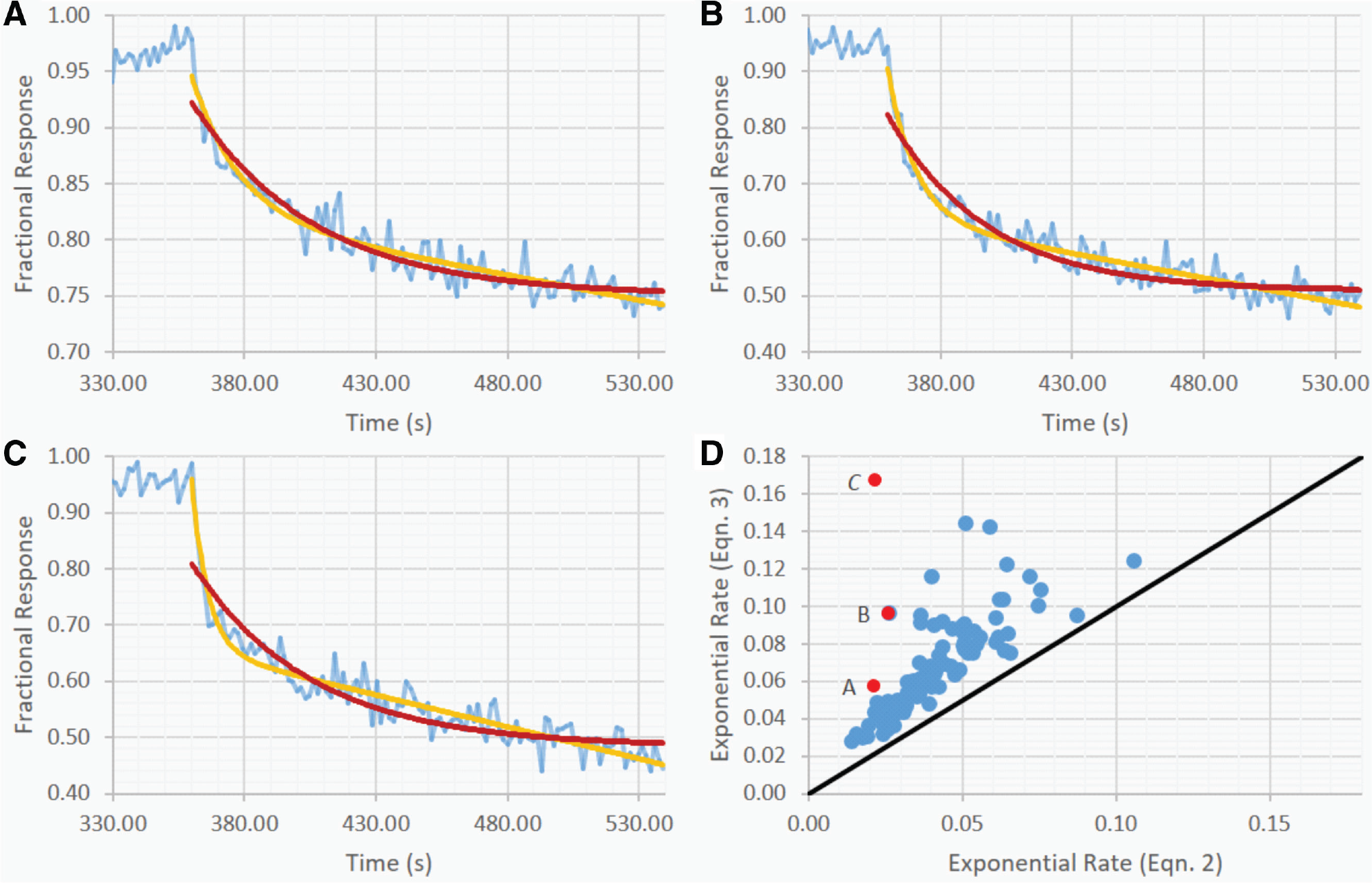
Model comparison for dissociation rate determination. Kinetic data were collected on an Octet HTX in high-throughput mode. Fits of the dissociation data (blue line) for mAbs A, B, and C, using the deconvolution model (yellow line) and the “partial-fit” model (red line), are shown for direct comparison (A–C, respectively) for outliers (red circles) of the correlated data (D).

Association Rate Deconvolution Using Fixed k_d

The observed association phase in suboptimal conditions may have a response convolved with signal contributions from aggregation of analyte on the sensor or nonspecific binding of proteins from direct exposure to culture supernatant. Additional complications include the consideration of the dissociation rates of each compound that may be binding specifically or nonspecifically to the sensor, sensor saturation, and the mass transport limitation ⁴ inherent to the ForteBio BLI platform. Conversely, the response in the dissociation phase is significantly cleaner with signal contributions originating only from molecules releasing from the sensor, assuming infinite dilution of material upon dissociation. With high confidence in the ability to extract k_d from dissociation phases and relatively low confidence in accurately extracting k_a, the former is used as a fixed parameter when globally fitting the data with equations (1) and (2) or equations (1) and (3). The result is the extracted requisite k_a for the k_d parameter to be representative of the data given the concentration of analyte and the raw signal. Data for mAbs A, B, and C were fit in this manner ( Fig. 2A–C ). All three mAbs association phases show a biphasic response with an apparent convolved slow phase of varying amplitude across the samples, which, through the method presented here, is ignored in the extracted k_a parameter. For comparison, this approach was also applied to an additional mAb, which was not an outlier in the correlation, mAb D ( Fig. 1D ), that shows minimal contribution of a slow phase in the association response ( Fig. 2D ). Likewise, the extracted k_a appears to be representative of the observed association phase as indicated by the agreement of the fit with the raw data.

Figure 2.

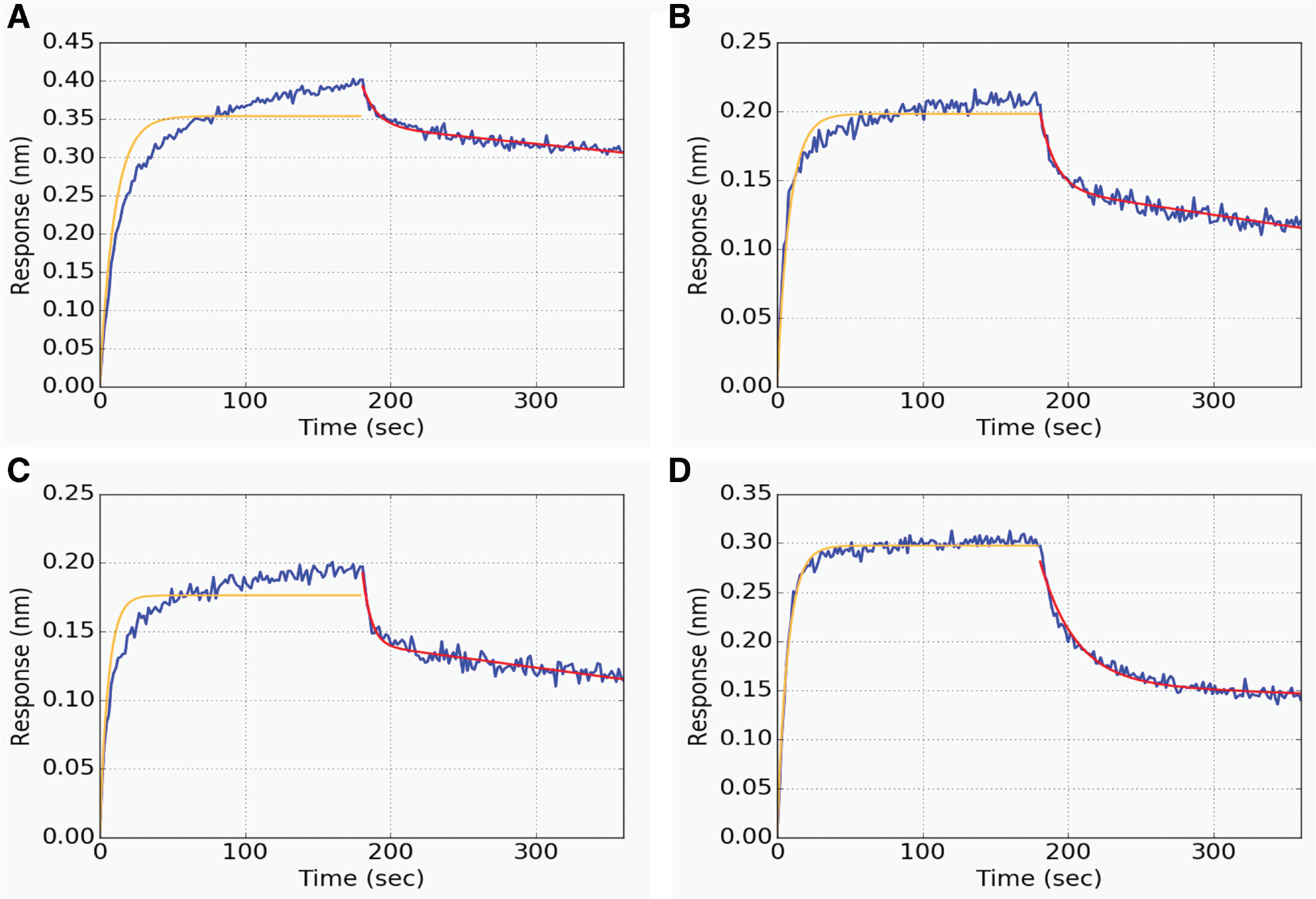
Deconvolution of association rates. Raw data for outlier mAbs A (k_a = 1.19E6 M⁻¹ s⁻¹, k_d = 0.051 s⁻¹), B (k_a = 5.14E5 M⁻¹ s⁻¹, k_d = 0.076 s⁻¹), and C (k_a = 2.24E5 M⁻¹ s⁻¹, k_d = 0.150 s⁻¹) are plotted, respectively. mAb D (k_a = 1.76E6 M⁻¹ s⁻¹, k_d = 0.035 s⁻¹) is included as an example data set that did not trigger the use of the linear approximation (D). The dissociation phases were fit (red line) to extract k_d, which was subsequently held constant for the deconvolution of k_a (orange line).

Binning Deconvolution and Detection of Allosteric Effectors

Epitope binning with kinetic competition experiments requires two molecules that bind to a single target molecule. Any combination, with respect to sensor orientation of the three molecules, can be used to observe kinetic competition, the most challenging of which is when a low-affinity interaction is used in the primary binding interaction. This may be the case when the desired properties to a specific target require low affinities or during early surveys within the discovery process ( Fig. 3 , mAb E). The optimal orientation requires immobilizing the higher affinity interaction on the sensor to interrogate the weaker interaction ( Fig. 3 , mAb F). However, in practice, both interactions may be relatively low affinity for the experimental time scale or when conducting the experiment with mAbs captured from culture supernatant, a process that generally requires the lower affinity interaction to be immobilized on the tip. In addition, when a noncontrol interaction is immobilized on the tip, the affinities of the primary interactions will all vary. The technical obstacle to having the lower affinity interaction bound to the tip is that, over time, the capacity for binding the second interaction will significantly decrease due to the dissociation kinetics of the primary interaction, resulting in a convolved secondary response. This is complicated further by having a multitude of affinities in the primary interactions such that any single amplitude cutoff cannot reliably be used. Without correcting the secondary response with the kinetics of the primary interaction, the convolved amplitude response may not appear positive, resulting in erroneous assignment of kinetic competition ( Fig. 3 , mAb E), making the data difficult to interpret with arbitrary cutoff values alone. Employing cutoff values without consideration for the kinetics of the primary interaction can lead to misidentification of a kinetic noncompetitor as a competitor ( Fig. 3A ). Correction of the binning data with the measured kinetic responses of the primary interaction and consideration for the ratio of molecular weights of each molecule with respect to the primary analyte can substantially improve the accuracy and consistency of such calls by converting the otherwise arbitrary scale to an absolute scale of percent bound with respect to the primary analyte concentration on the sensor ( Fig. 3C ). An additional benefit to this analysis is the facile detection of kinetic competitors that are epitopically distinct but allosterically coupled^19,20 ( Fig. 3 , mAb G), which is possible to obtain without further experiments.

Figure 3.

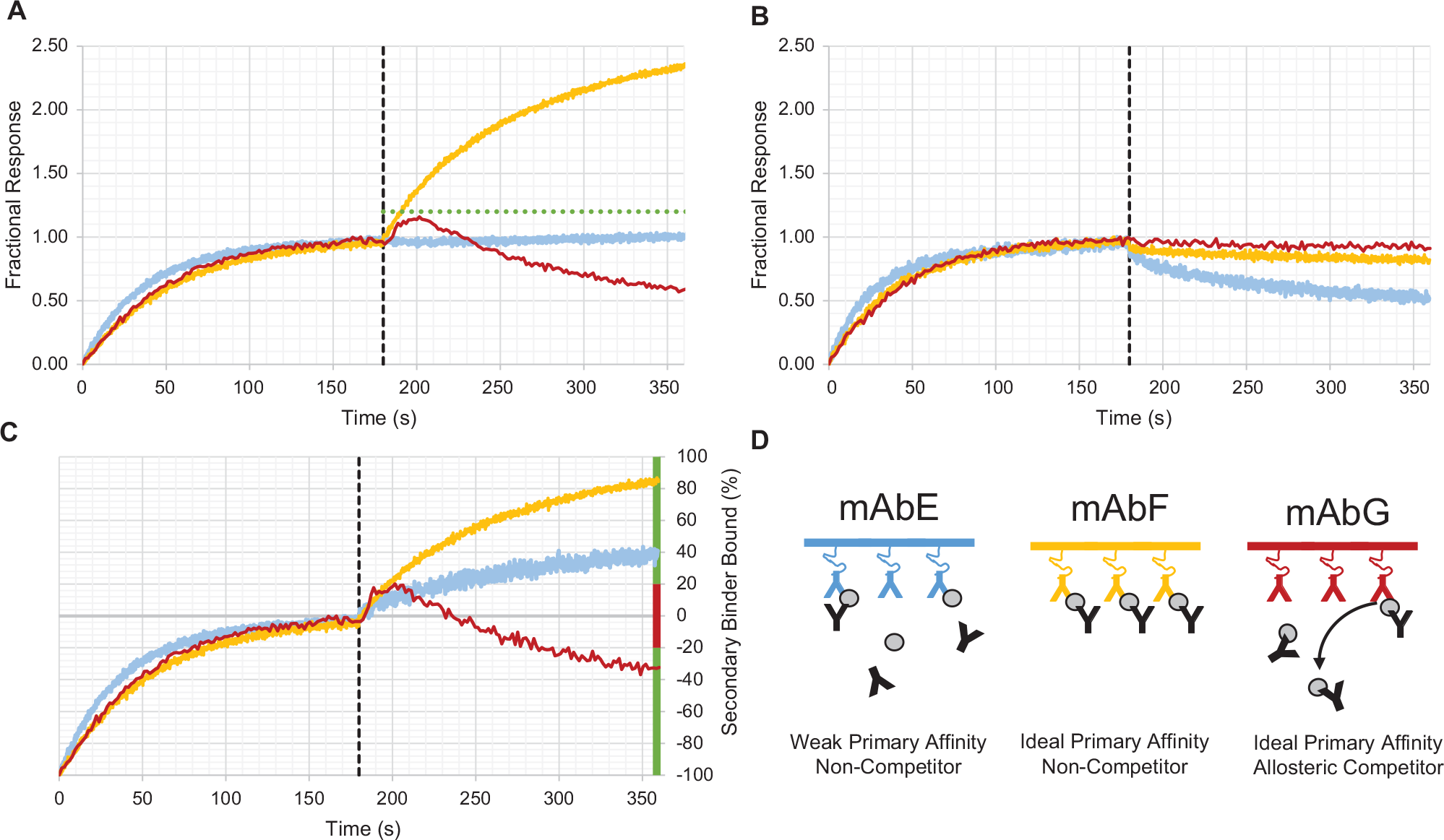
Kinetic correction of binning data. Normalized binning data with respect to the association phase (A) is typically evaluated with an arbitrary response cutoff (green dotted line). Kinetic data of the primary interaction are queried from the database and normalized (B). Correction of the binning data by subtraction of the kinetic data and scaling of binning step by the relative molecular weights transform the y-axis to percent bound of available antigen on the sensor (C). An absolute scale is used to determine if the binning response is indicative of no kinetic competition (green vertical bar, positive values) or kinetic competition (red vertical bar). Kinetic competition can be either epitopic (red vertical bar) or allosteric (green vertical bar, negative values) in nature, using a 20% bound cutoff for epitopic competition. The association and binning steps are indicated by the t₀ of the latter phase (dashed black line). Schematic model representation for each kinetic interaction is coded by color of the kinetic plots (D).

In conclusion, recent advances in biosensor-based molecular binding kinetics instrumentation has focused on hardware improvements for signal resolution and throughput. The volume of data that these instruments produce presents challenges so far unaddressed by commercial software solutions, including the efficient handling of large volumes of data with respect to both speed and analytical utility. In parallelized industrial settings, these limitations produce compounded inefficiencies. The database-centric method presented in this work overcomes these obstacles by providing relevant historical data on demand, defining a new analytical model to account for nonspecific interactions, describing an algorithm for appropriate model selection to adjust the analysis to the data quality, outlining the correction of data for unambiguous cutoff determinations, improving analytical insight with the detection of allosteric effectors, and providing a high-throughput automated analytical solution.