Sage Journals: Discover world-class research

Abstract

Differential evolution (DE) has been applied extensively in drug combination optimization studies in the past decade. It allows for identification of desired drug combinations with minimal experimental effort. This article proposes an adaptive population-sizing method for the DE algorithm. Our new method presents improvements in terms of efficiency and convergence over the original DE algorithm and constant stepwise population reduction–based DE algorithm, which would lead to a reduced number of cells and animals required to identify an optimal drug combination. The method continuously adjusts the reduction of the population size in accordance with the stage of the optimization process. Our adaptive scheme limits the population reduction to occur only at the exploitation stage. We believe that continuously adjusting for a more effective population size during the evolutionary process is the major reason for the significant improvement in the convergence speed of the DE algorithm. The performance of the method is evaluated through a set of unimodal and multimodal benchmark functions. In combining with self-adaptive schemes for mutation and crossover constants, this adaptive population reduction method can help shed light on the future direction of a completely parameter tune-free self-adaptive DE algorithm.

Keywords

differential evolution self-adaptation population size global optimization artificial intelligence

Introduction

Differential evolution (DE) is a simple, reliable, and efficient population-based real-parameter function optimizer derived from the evolutionary algorithm (EA).^1–4 A number of studies have pointed out that compared with other evolutionary-based algorithms, DE is more practical and exhibits much better performance on a wide variety of problems.^5–9 Recently, the DE algorithm has been applied in combinatorial drug studies, in which multiple drugs with multiple dose levels are present and an optimal drug combination is required to develop desired treatment efficacy. To identify the optimal drug combinations from a large pool of drug candidates is traditionally considered a tedious and prohibitive task. With the advancement of technology in the emerging interdisciplinary field of combinatorial drug optimization, feedback system control strategies that were conventionally applied mainly in the engineering domain have gradually been adapted for biological complex systems. The hybrid of biological experimental advancements and engineering optimization platforms has paved the way for a paradigm shift for new drug development in various disease models.^10–16 For instance, Ding et al.¹⁵ applied DE to identify the optimal drug combination to treat herpes simplex virus type 1 (HSV-1). Nowak-Sliwinska et al.¹⁶ demonstrated the application of DE to identify the optimal drug combination to treat cancer angiogenesis. Tsutsui et al.¹⁷ adopted DE in their effort to identify the optimal drug combinations for long-term maintenance of human embryonic stem cells. Honda . et al.¹⁸ proved DE could quickly provide a solution to control the osteogenesis process of human mesenchymal stem cells. The success of DE is found to be due to an implicit self-adaptation contained within the algorithmic structure, which makes it highly explorative at the beginning of the evolution and subsequently becomes more exploitative in the later stage of the optimization.¹⁹

The simplicity, ease of implementation, and the great performance of DE in terms of accuracy, convergence speed, and robustness make it attractive for a diverse domain of real-world optimization problems. DE has been extensively applied in engineering fields such as robotics,⁵ electronics,²⁰ engineering,²¹ financial planning,²² risk management,²³ and medical applications.²⁴ A review of DE applications has been presented by Plagianakos et al.²⁵

Although it is clear to the scientific community that DE is a powerful global optimization algorithm, there still remains considerable margin of improvement. This triggered extensive research efforts over the past decade, resulting in a wealth of variants designed to improve the performance of the original DE.^5,6

The performance of the original DE algorithm is mainly affected by three control parameters: the mutation factor F, the crossover constant CR, and the population size NP. Because these values have to be tuned to fit specific optimization applications, a major problem that researchers face is the choice of a right set of control parameters. This problem is amplified when DE is employed for handling various difficulties in real-world applications such as high dimensionality and noisy optimization problems. In view of this, a wealth of DE variants has been proposed to improve the robustness and efficiency through the application of adaptive or self-adaptive techniques.^26–30

Neri and Tirronen⁵ suggested that, among a selection of DE variants, population size reduction, dynNP-DE, proposed by Brest and Maucec,³¹ is one of the most effective algorithmic components in terms of robustness and efficiency, whereas the self-adaptive control parameter scheme (jDE) proposed by Brest and Maucec³² is superior in terms of robustness and versatility over a diverse benchmark functions.

In this work, we propose a new population reduction method that can dynamically and continuously reduce the population size in response to the optimization progress. Our new method presents improvements in terms of efficiency and convergence over dynNP-DE. The method is DE structure independent, so it can be integrated into any type of DE variant.

This article is organized as follows. The next section reviews the background of the original DE algorithm and surveys recent work on different variants of DE. The third section describes the mechanism of the self-adaptive control parameter DE scheme. The section also provides the detailed mechanism and properties of our new population-based method, which we termed the continuous adaptive population reduction (CAPR) method. The fourth section presents experimental results on the comparisons of the performance between our new method and the well-studied population reduction scheme dynNP-DE, by testing with well-known benchmark functions under a wide range of dimensions. The fifth section discusses the experimental results. The sixth section concludes this work.

Related Works

Most of the DE variants proposed in the literature are based on either adaptation or self-adaptation of the crossover and mutation rate, namely, F and CR.^{26,29,32–35} These variants of DE have been shown to greatly improve the robustness and efficiency by dynamically adjusting the control parameters.

Liu and Lampinen³³ proposed a fuzzy adaptive DE algorithm that uses fuzzy logic controllers to adapt the search parameters for the mutation and crossover operations. Brest et al.²⁷ proposed a self-adaptive scheme (jDE) in which the control parameters F and CR are assigned to each agent in the population. Better agents, resulted from better control parameters, are more likely to produce better offspring to survive the selection process. These offspring in turn enhance the likelihood for the better parameter values to propagate. Das et al.³⁶ modified the original mutation scheme in DE by involving both global and local neighbors, which are defined as the entire population and a portion of the nearby agents in the population, respectively. The combined contributions between these two parts are weighted self-adaptively. Neri and Tirronen³⁵ proposed a scale factor local search DE, which applied a local search with certain probability to the scale factor F, corresponding to the offspring with higher performance, during the generation of an offspring.

Besides the variants that focused on the adaptation and self-adaptation of the control parameters, others focused on the adaptation of various mutation strategies or hybridization with other strategies. Fan and Lampinen³⁷ proposed the trigonometric differential evolution (TDE) in which the mutation operation is replaced by a trigonometric mutation scheme with a prefixed probability. Qin and Suganthan²⁹ proposed a self-adaptive DE (SaDE) algorithm in which different mutation strategies are allowed to switch between each other while F and CR are allowed to self-adapt without any predefinition. Rahnamayan et al.³⁸ proposed an opposition-based DE that applies the logic of opposition points to generate initial population. The method improves the convergence properties of DE on noisy and large-scale problems. Mezura-Montes et al.³⁹ conducted a comparison study on the different DE variants.

Besides controlling the mutation and crossover parameters, it should be obvious that varying the population size during the optimization process could also be a highly rewarding approach. However, population size has so far not been studied as much as the other two control parameters. In contrast, in the context of EAs, population-sizing schemes have long been investigated in a number of works, such as Genetic Algorithm with Varying Population Size (GAVaPS),⁴⁰ Adaptive Population size Genetic Algorithm,⁴¹ Random Variation of Population Size GA,⁴² and Population Resizing on Fitness Improvement GA.⁴³ Lobo and Lima⁴⁴ surveyed a variety of population-sizing schemes for EAs.

The effect of population size NP on the DE algorithm is analogous to the EAs in which too small a population could cause premature convergence and too large a population could lead to stagnation.⁴⁵ In the context of DE, there exist a few works that focused on the population size. Teo³⁴ made the first attempt by self-adapting NP using an absolute and relative encoding scheme which was improved by Teng et al.⁴⁶ Neri et al.²⁴ proposed an integration of fitness diversity into the DE structure where population size and the other parameters encoded within each agent are self-adapted based on a measurement of the fitness diversity. Brest and Maucec³¹ proposed a population size reduction scheme in which the population size is reduced in a stepwise fashion during the optimization process, so as to avoid DE stagnation with high dimensional problems. The idea is shown to significantly improve robustness for large-scale problems.^31,47

In addition, several new variants of population-resizing mechanisms have been proposed recently in the framework of DE. Zhang et al.⁴⁸ recently incorporated the lifetime and extinction mechanisms of GaVAPS to regulate the population size in an adaptive manner. Dziedzic⁴⁹ proposed a clustering-based population size reduction method in which only the best specimens from each of the resulting clusters are transferred to the next generation. Wang and Zhao⁵⁰ proposed a self-adaptive population-resizing mechanism, SapsDE, in which the population size can be adjusted dynamically by eliminating a fixed amount of poorest performing population based on some online solution-search status. Zamuda et al.⁵¹ proposed a structured population size reduction algorithm in which dynNP-DE is combined with multiple population size–dependent mutation strategies using a structured population.

DE and Related Algorithms

DE is a stochastic, population-based algorithm developed for real-valued function optimization problems.² It operates by having a population of agents (x vector) that move around in the search space by recombining through crossover and mutation with other existing agents in the population. Through an aggressive selection process, a newly generated agent is accepted as part of the population if the new agent x is an improvement; otherwise, it is discarded. This iteration process is repeated to find a vector x that optimizes a function f (x).

A brief description of the original DE algorithm² iteration procedures is as follows:

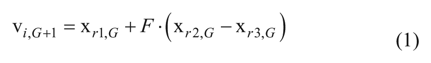
Generate a population of D-dimensional target vectors x_i,G = {x_1i,G, x_2i,G, . . . , x_Di,G}, i = 1, 2, . . . , NP from the solution space S. D is the dimensionality of the function f. S ⊆ R^D is the D-dimensional search space for the problem. NP is the population size, and G is the iterative generation. The initial population is selected randomly from a uniform distribution between upper and lower bounds, x_j,low and x_j,upp, defined for each variable x_j, j ∈{1, . . . , D}.

Generate a trial vector u_i,G+1 for each vector x_i,G in turn by employing mutation, crossover, and selection procedures as follows, until either a value to reach (VTR) or maximum number function evaluations (MaxFES) criterion is reached:

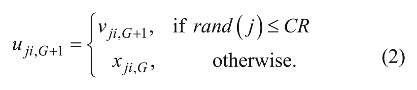
Mutation: Generate a mutant vector v_i,G using DE/rand/1 strategy for each vector x_i,G:

v_{i, G + 1} = x_{r 1, G} + F \cdot (x_{r 2, G} - x_{r 3, G})

where r1, r2, r3 ∈{1, . . . , NP} are random indexes and are mutually different from each other and i. F is the amplification factor ∈[0, 1], which controls the amplification of the differential variation (x_r2,G – x_r3,G).

Crossover: Perform binomial crossover:

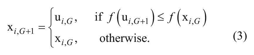
u_{j i, G + 1} = {\begin{matrix} v_{j i, G + 1}, if r a n d (j) \leq C R \\ x_{j i, G}, otherwise . \end{matrix}

where CR is the crossover control parameter.

Selection: Perform selection between the trial vector and target vector using a greedy selection criterion:

x_{i, G + 1} = {\begin{cases} u_{i, G}, if f (u_{i, G + 1}) \leq f (x_{i, G}) \\ x_{i, G}, otherwise . \end{cases}

Output the results of the best target vector.

Self-adaptive DE algorithms eliminate the manual tuning of F and CR for different types of functions. To facilitate the sole comparison with an existing dynamic population reduction algorithm, we used the same self-adaptive schemes and parameter settings as presented in Brest et al.⁵² This self-adaptive scheme has been shown to provide enhanced robustness and great performance for large-scale problems,⁴⁸ constrained optimization,⁵³ and multi-objective problems⁵⁴ and has been extensively discussed.^5,6

The method allows a self-tuning of the control parameters, F and CR, of each individual agent in the population in each iteration. F_i,G+1 and CR_i,G+1 are updated according to the following scheme:

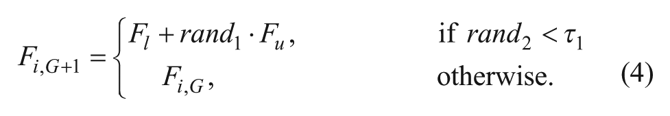
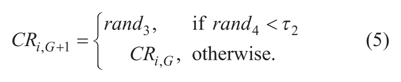
F_{i, G + 1} = {\begin{matrix} F_{l} + r a n d_{1} \cdot F_{u}, if r a n d_{2} < τ_{1} \\ F_{i, G}, otherwise . \end{matrix}

C R_{i, G + 1} = {\begin{matrix} r a n d_{3}, if r a n d_{4} < τ_{2} \\ C R_{i, G}, otherwise . \end{matrix}

where rand_j, j∈{1, 2, 3, 4}, are uniformly distributed random values between 0 and 1; τ₁ and τ₂ are constant values, 0.1, which represent the probabilities that the control parameters F and CR are updated, respectively. F_l and F_u are constant values, 0.1 and 0.9, respectively, which represent the minimum and maximum values that F can take. This allowed F_i,G+1 and CR_i,G+1 to take a value from [0.1, 1.0] and [0, 1], respectively, in a random manner. These parameters are renewed before each trial vector generation and are used during the mutation, crossover, and selection steps during the creation of each offspring x_i,G+1.

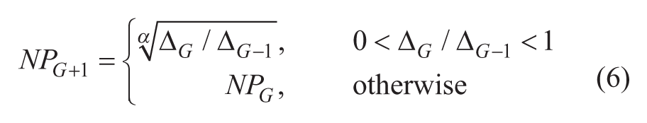
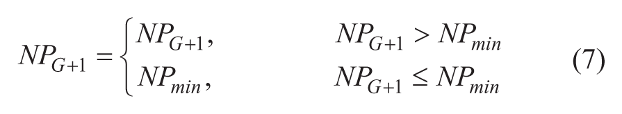
In this section, we introduce our CAPR scheme. We have mentioned in the previous section that two control parameters, F and CR, can be self-adapted within each individual agent during each iteration run, through a self-adaptive DE scheme (jDE).²⁷ To further improve the efficiency of the DE algorithm, we propose a new dynamic population size reduction scheme that eliminates the manual tuning of the third control parameter, NP. The method gradually reduced the population size according to the change of gradient of the fitness value. A new NP is calculated after one cycle of function evaluations for all agents in the population:

N P_{G + 1} = {\begin{matrix} \sqrt[α]{Δ_{G} / Δ_{G - 1}}, 0 < Δ_{G} / Δ_{G - 1} < 1 \\ N P_{G}, otherwise \end{matrix}

N P_{G + 1} = {\begin{matrix} N P_{G + 1}, N P_{G + 1} > N P_{m i n} \\ N P_{m i n}, N P_{G + 1} \leq N P_{m i n} \end{matrix}

where

Δ_{G} = \frac{f_{a v e} (x_{G}) - f_{a v e} (x_{G - 1})}{f_{a v e} (x_{G})}, Δ_{G - 1} = \frac{f_{a v e} (x_{G - 1}) - f_{a v e} (x_{G - 2})}{f_{a v e} (x_{G - 1})}

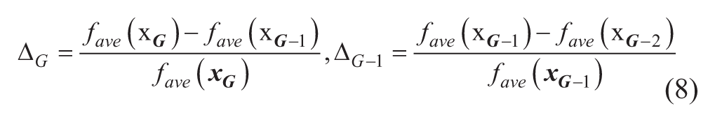
After one cycle of evaluation of all agents in the population (i.e., NP_G function evaluations), the evaluated function values of all agents in the population are averaged to be f _ave(x_G). This value, together with that from the previous evaluation cycle, is used to calculate the normalized gradient value ∆_G (8). Δ_G-1 is calculated in a similar fashion using the previous average function evaluation value, f_ave(x_G-1), and the one before the previous, f_ave(x_G-2). If the ratio Δ_G/Δ_G-1 is within the range of [0, 1], then NP is reduced by a fraction equal to the α-th root of the ratio of Δ_G/Δ_G-1. The reason for taking a root of the ratio is to slow down the population size reduction rate. Unless stated otherwise, the parameter α takes a value of 100.

The design behind our population reduction scheme was inspired by dynNP-DE proposed by Brest and Maucec.³¹ In their method, population reduction was performed in a stepwise fashion a few times throughout the whole optimization process. The numbers of function evaluations are distributed evenly for each population size. More specifically, the algorithm was predefined to reduce the population by pmax number of times. After each size reduction, the new population size is always equal to half of the previous population size. During the population reduction, one individual from each half of the current population is compared based on their fitness values, and the better one becomes the survivor for the next generation. For example, if the total number of function evaluations is predefined as 100,000, pmax = 4, and initial population = 200, the population size for each generation will be NP_i ∈ {200, 100, 50, 25}, and each generation will last for 100,000/pmax/NP_i = {125, 250, 500, 1000} number of function evaluations. This stepwise population size reduction mechanism allows us to wonder about the possibility of a continuous, instead of stepwise, population size reduction scheme that may more efficiently and interactively reduce the population size.

In CAPR, the population size reduction rate is dependent on the gradient of optimization performance. Compared with dynNP-DE, in which the population is always reduced by half of the previous population for a predefined number of times, the population reduction size in CAPR is not a constant but a variable based on the performance of the current and previous iterations. The population is reduced only if the gradient of the current generation, Δ_G, is lower than the gradient of the previous generation, Δ_G-1. As is for all population-based evolutionary algorithms, a large pool of diverse populations is required at the beginning of the optimization process for exploration reasons. In the later stages of the evolutionary process, exploitation should take place to improve the best-so-far individuals. Exploitation should start only when exploration starts to slow down. Therefore, an increase in the gradient simply means the optimization process is still in the exploration phase, and therefore, reduction of population size should not be carried out. For the same reason, if the current gradient has an opposite sign of the previous gradient, which means the performance of the current iteration is worse than the previous iteration, the population will also not be reduced.

Moreover, because of the fast population reduction rate of CAPR, we do not perform any sorting or comparison, which keeps only the best individuals in the reduced NP population. Instead, we simply randomly truncate the excessive agents in the population. This prevents the method from always picking the best individuals, which may trap the optimization into local optimum. This also avoids any addition on the time complexity to the algorithm.

We have limited the minimum population size, NP_min, to be the same as the dimension. This is higher than the minimum requirement of standard DE, which is 4 (r1, r2, r3, and i itself), for the crossover step. We found that the higher NP_min is helpful to our algorithm. As we will notice in the later sections, our algorithm indeed reduces the population quite fast ( Figs. 1 and 2 ), and thus a higher NP_min could help to reduce the chance of being trapped in local optimum.

Figure 1.

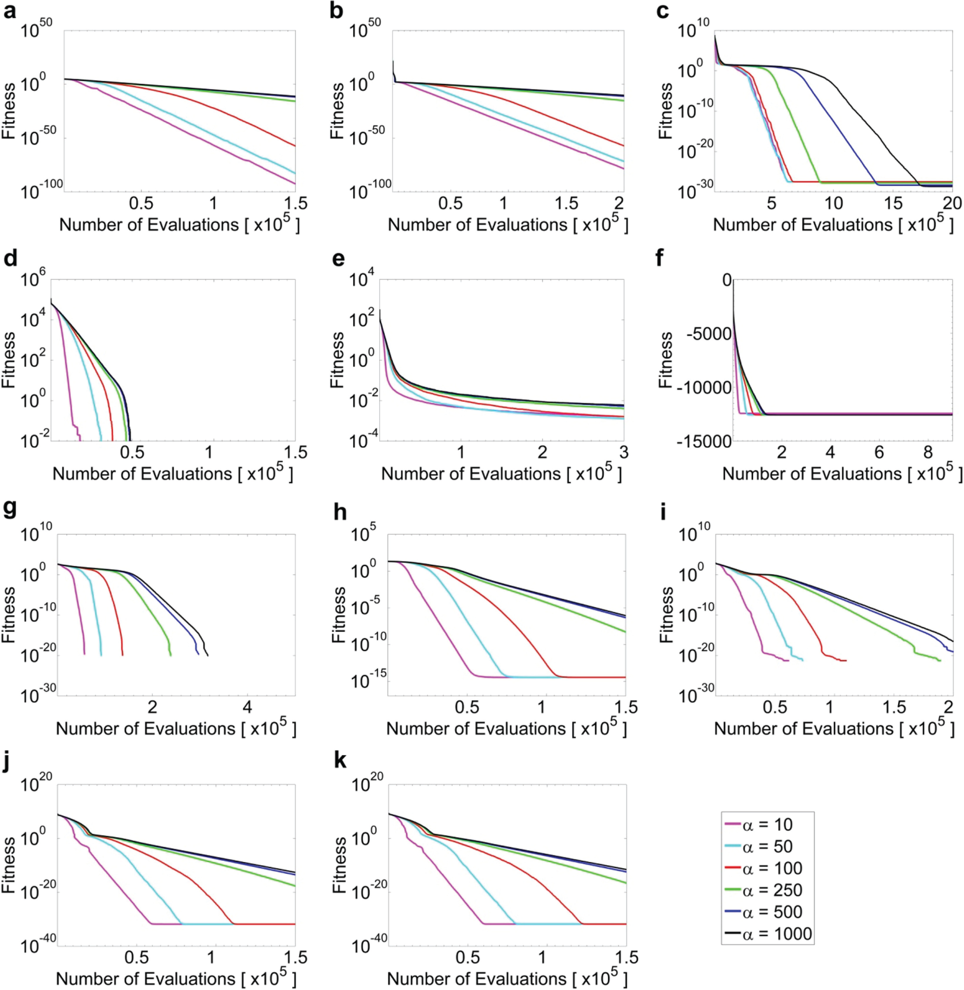
Average fitness value of all performing agents averaged over 100 independent experiments for f₁ (a), f₂ (b), f₅ (c), f₆ (d), f₇ (e), f₈ (f), f₉ (g), f₁₀ (h), f₁₁ (i), f₁₂ (j), and f₁₃ (k) at D = 30 at different α values (see legends).

Figure 2.

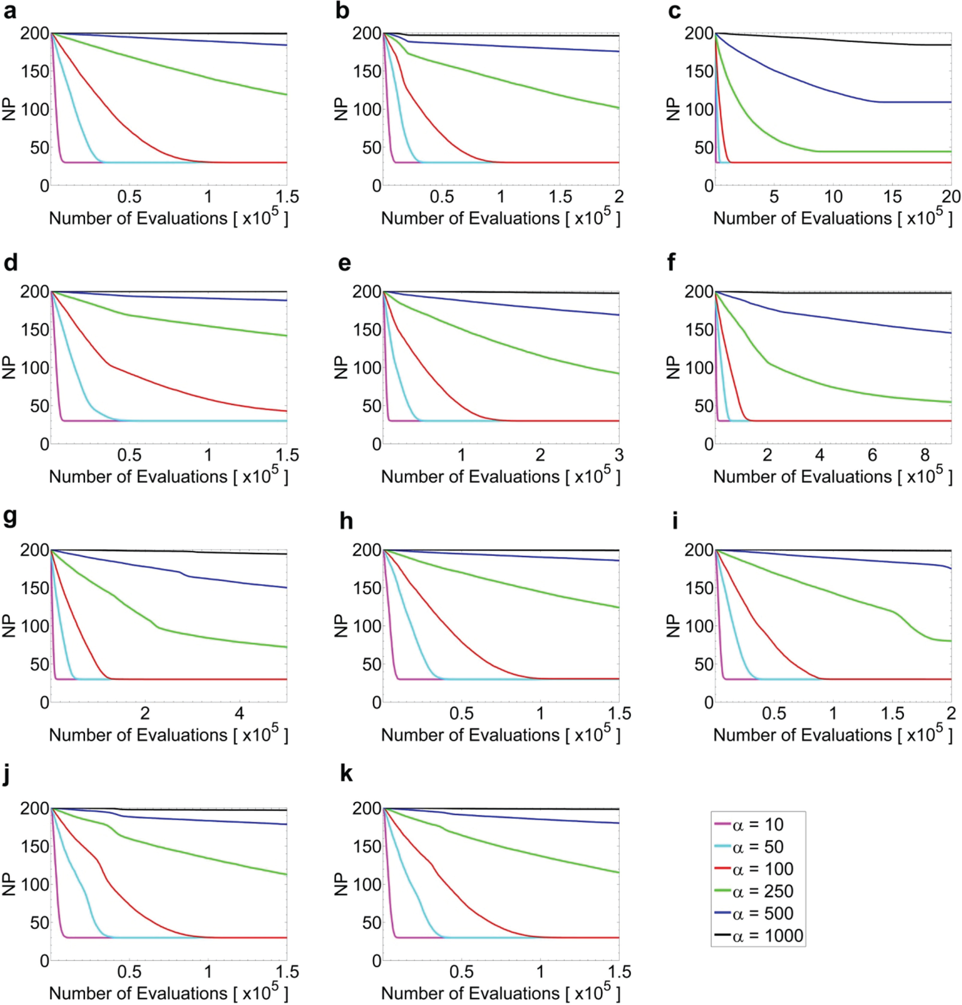
Average population size of all performing agents averaged over 100 independent experiments for f₁ (a), f₂ (b), f₅ (c), f₆ (d), f₇ (e), f₈ (f), f₉ (g), f₁₀ (h), f₁₁ (i), f₁₂ (j), and f₁₃ (k) for D = 30 at different α values (see legends).

One should notice that our population reduction scheme is designed only for reducing the population and not increasing the population. It is certainly possible to increase the population size by a certain amount if the evolutionary process is not able to improve the optimization after a long quiescent period. In this present work, we did not investigate this aspect and would like to focus solely on the population size reduction mechanism.

Results

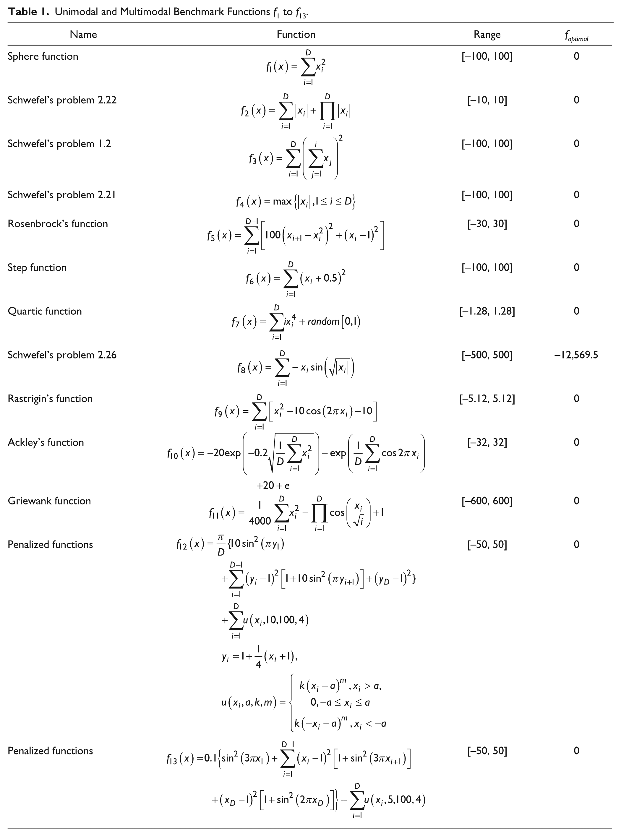
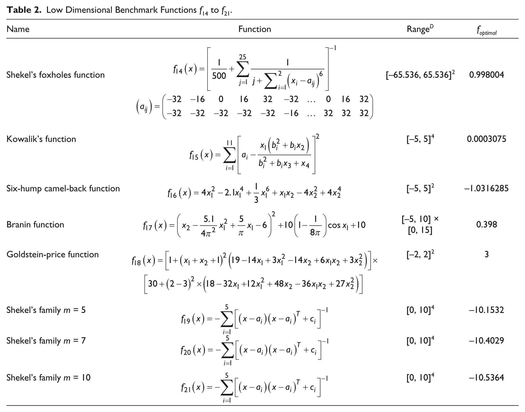
Our algorithm was tested with 21 benchmark functions shown in Tables 1 to 3 . The functions are numbered as in Brest and Maucec³¹ for comparison purposes with dynNP-DE. More detailed properties of each function can be found in Yao et al.⁵⁴ Functions f₁ to f₁₃ are scalable to high dimensions. Functions f₁ to f₅ are unimodal functions. Function f₆ is a step function with one minimum and is discontinuous. Function f₇ is a noisy quartic function, where rand[0, 1) is a uniformly distributed random variable in [0, 1). Functions f₈ to f₁₃ are multimodal functions in which the number of local minima increases exponentially with the problem dimension. These functions appear to be the most difficult class of problems for many optimization algorithms.⁵⁴ We also tested some low-dimensional functions, f₁₄ to f₂₁, which have only a few local minima. All experimental results and figures presented are averaged over 100 independent runs.

Table 1.

Unimodal and Multimodal Benchmark Functions f₁ to f₁₃.

Name	Function	Range	f_optimal
Sphere function	$f_{1} (x) = \sum_{i = 1}^{D} x_{i}^{2}$	[−100, 100]	0
Schwefel’s problem 2.22	$f_{2} (x) = \sum_{i = 1}^{D} \| x_{i} \| + \prod_{i = 1}^{D} \| x_{i} \|$	[−10, 10]	0
Schwefel’s problem 1.2	$f_{3} (x) = \sum_{i = 1}^{D} {(\sum_{j = 1}^{i} x_{j})}^{2}$	[−100, 100]	0
Schwefel’s problem 2.21	$f_{4} (x) = \max {\| x_{i} \|, 1 \leq i \leq D}$	[−100, 100]	0
Rosenbrock’s function	$f_{5} (x) = \sum_{i = 1}^{D - 1} [100 {(x_{i + 1} - x_{i}^{2})}^{2} + {(x_{i} - 1)}^{2}]$	[−30, 30]	0
Step function	$f_{6} (x) = \sum_{i = 1}^{D} {(x_{i} + 0.5)}^{2}$	[−100, 100]	0
Quartic function	$f_{7} (x) = \sum_{i = 1}^{D} i x_{i}^{4} + r a n d o m [0, 1)$	[−1.28, 1.28]	0
Schwefel’s problem 2.26	$f_{8} (x) = \sum_{i = 1}^{D} - x_{i} \sin (\sqrt{\| x_{i} \|})$	[−500, 500]	−12,569.5
Rastrigin’s function	$f_{9} (x) = \sum_{i = 1}^{D} [x_{i}^{2} - 10 \cos (2 π x_{i}) + 10]$	[−5.12, 5.12]	0
Ackley’s function	$\begin{array}{l} f_{10} (x) = - 20 \exp (- 0.2 \sqrt{\frac{1}{D} \sum_{i = 1}^{D} x_{i}^{2}}) - \exp (\frac{1}{D} \sum_{i = 1}^{D} \cos 2 π x_{i}) \\ + 20 + e \end{array}$	[−32, 32]	0
Griewank function	$f_{11} (x) = \frac{1}{4000} \sum_{i = 1}^{D} x_{i}^{2} - \prod_{i = 1}^{D} \cos (\frac{x_{i}}{\sqrt{i}}) + 1$	[−600, 600]	0
Penalized functions	$\begin{array}{l} f_{12} (x) = \frac{π}{D} {10 \sin^{2} (π y_{1}) \\ + \sum_{i = 1}^{D - 1} {(y_{i} - 1)}^{2} [1 + 10 \sin^{2} (π y_{i + 1})] + {(y_{D} - 1)}^{2}} \\ + \sum_{i = 1}^{D} u (x_{i}, 10, 100, 4) \\ y_{i} = 1 + \frac{1}{4} (x_{i} + 1), \\ u (x_{i}, a, k, m) = {\begin{matrix} k {(x_{i} - a)}^{m}, x_{i} > a, \\ 0, - a \leq x_{i} \leq a \\ k {(- x_{i} - a)}^{m}, x_{i} < - a \end{matrix} \end{array}$	[−50, 50]	0
Penalized functions	$\begin{array}{l} f_{13} (x) = 0.1 {\sin^{2} (3 π x_{1}) + \sum_{i = 1}^{D - 1} {(x_{i} - 1)}^{2} [1 + \sin^{2} (3 π x_{i + 1})] \\ + {(x_{D} - 1)}^{2} [1 + \sin^{2} (2 π x_{D})]} + \sum_{i = 1}^{D} u (x_{i}, 5, 100, 4) \end{array}$	[−50, 50]	0

Table 2.

Low Dimensional Benchmark Functions f₁₄ to f₂₁.

Name	Function	Range^D	f_optimal
Shekel’s foxholes function	$f_{14} (x) = {[\frac{1}{500} + \sum_{j = 1}^{25} \frac{1}{j + \sum_{i = 1}^{2} {(x_{i} - a_{i j})}^{6}}]}^{- 1}$ $(a_{i j}) = (\begin{matrix} - 32 & - 16 & 0 & 16 & 32 & - 32 & \dots & 0 & 16 & 32 \\ - 32 & - 32 & - 32 & - 32 & - 32 & - 16 & \dots & 32 & 32 & 32 \end{matrix})$	[−65.536, 65.536]²	0.998004
Kowalik’s function	$f_{15} (x) = \sum_{i = 1}^{11} {[a_{i} - \frac{x_{1} (b_{i}^{2} + b_{i} x_{2})}{b_{i}^{2} + b_{i} x_{3} + x_{4}}]}^{2}$	[−5, 5]⁴	0.0003075
Six-hump camel-back function	$f_{16} (x) = 4 x_{1}^{2} - 2.1 x_{1}^{4} + \frac{1}{3} x_{1}^{6} + x_{1} x_{2} - 4 x_{2}^{2} + 4 x_{2}^{4}$	[−5, 5]²	−1.0316285
Branin function	$f_{17} (x) = {(x_{2} - \frac{5.1}{4 π^{2}} x_{1}^{2} + \frac{5}{π} x_{1} - 6)}^{2} + 10 (1 - \frac{1}{8 π}) \cos x_{1} + 10$	[−5, 10] × [0, 15]	0.398
Goldstein-price function	$f_{18} (x) = [1 + {(x_{1} + x_{2} + 1)}^{2} (19 - 14 x_{1} + 3 x_{1}^{2} - 14 x_{2} + 6 x_{1} x_{2} + 3 x_{2}^{2})] \times [30 + {(2 - 3)}^{2} \times (18 - 32 x_{1} + 12 x_{1}^{2} + 48 x_{2} - 36 x_{1} x_{2} + 27 x_{2}^{2})]$	[−2, 2]²	3
Shekel’s family m = 5	$f_{19} (x) = - \sum_{i = 1}^{5} {[(x - a_{i}) {(x - a_{i})}^{T} + c_{i}]}^{- 1}$	[0, 10]⁴	−10.1532
Shekel’s family m = 7	$f_{20} (x) = - \sum_{i = 1}^{5} {[(x - a_{i}) {(x - a_{i})}^{T} + c_{i}]}^{- 1}$	[0, 10]⁴	−10.4029
Shekel’s family m = 10	$f_{21} (x) = - \sum_{i = 1}^{5} {[(x - a_{i}) {(x - a_{i})}^{T} + c_{i}]}^{- 1}$	[0, 10]⁴	−10.5364

Table 3.

Values of a_i and c_i for f₁₉ to f₂₁.

i	1	2	3	4	5	6	7	8	9	10
a_ij, j = 1, . . . ,4	4	1	8	6	3	2	5	8	6	7
	4	1	8	6	7	9	5	1	2	3.6
	4	1	8	6	3	2	3	8	6	7
	4	1	8	6	7	9	3	1	2	3.6
c_i	0.1	0.2	0.2	0.4	0.4	0.6	0.3	0.7	0.5	0.5

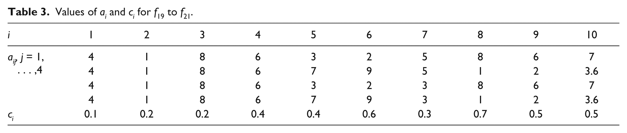
Table 4 presents the experimental results of our algorithm in comparison to dynNP-DE and the original DE algorithm with dimensions D = 30. To illustrate the sole effect caused by the population reduction algorithm, and to facilitate comparison with the dynNP-DE algorithm, we used the same self-adaptive schemes and parameter settings used in Brest and Maucec.³¹ Initial values of the self-adaptive control parameters, F = 0.5 and CR = 0.9; initial NP value, NP_init = 200; and α = 100 were used in most experiments in this work, unless stated otherwise. The minimum NP value is set to NP_min = 30, which is the same as the dimension size D.

Table 4.

Comparison between CAPR, dynNP-DE, and the Original DE in Experimental Results, when D = 30.^a

F	MaxFES	CAPR, Mean Best (SD)	dynNP-DE, Mean Best (SD)	Original DE, Mean Best (SD)
f ₁	150,000	2.17 × 10⁻⁵⁸ (1.68 × 10⁻⁵⁷)	4.04 × 10⁻⁴⁹ (3.76 × 10⁻⁴⁸)	8.31 × 10^−14b (4.46 × 10⁻¹⁴)
f ₂	200,000	2.0 × 10⁻⁵⁶ (1.59 × 10⁻⁵⁵)	3.53 × 10⁻⁴⁴ (2.15 × 10⁻⁴³)	1.60 × 10^−9b (1.17 × 10⁻⁹)
f ₅	2 × 10⁶	2.63 × 10⁻²⁷ (1.08 × 10⁻²⁶)	1.54 × 10^−28b (1.76 × 10⁻²⁸)	3.46 × 10⁻³¹ ^b (2.45 × 10⁻³⁰)
f ₆	150,000	0 (0)	0 (0)	0 (0)
f ₇	300,000	1.51 × 10⁻³ (4.05 × 10⁻⁴)	1.69 × 10^−3v (4.92 × 10⁻⁴)	8.63 × 10^−3b (1.72 × 10⁻³)
f ₈	900,000	–12,569.5 (7.23 × 10⁻¹⁴)	–12,569.5 (4.73 × 10⁻¹¹)	−11,148.5^b (4.96 × 10²)
‘F ₉	500,000	0 (0)	0 (0)	69.19^b (38.8)
f ₁₀	150,000	3.41 × 10⁻¹⁵ (0)	3.73 × 10^−15b (7.78 × 10⁻¹⁶)	9.71 × 10^−8b (3.51 × 10⁻⁸)
f ₁₁	200,000	0 (0)	0 (0)	2.82 × 10^−20b (4.80 × 10⁻²⁰)
f ₁₂	150,000	1.59 × 10⁻³² (2.07 × 10⁻³³)	1.92 × 10⁻³² (3.69 × 10⁻³²)	2.04 × 10^−7b (9.27 × 10⁻⁸)
f ₁₃	150,000	2.25 × 10⁻³² (3.74 × 10⁻³²)	3.40 × 10⁻³² (9.36 × 10⁻³²)	1.79 × 10^−6b (6.53 × 10⁻⁷)

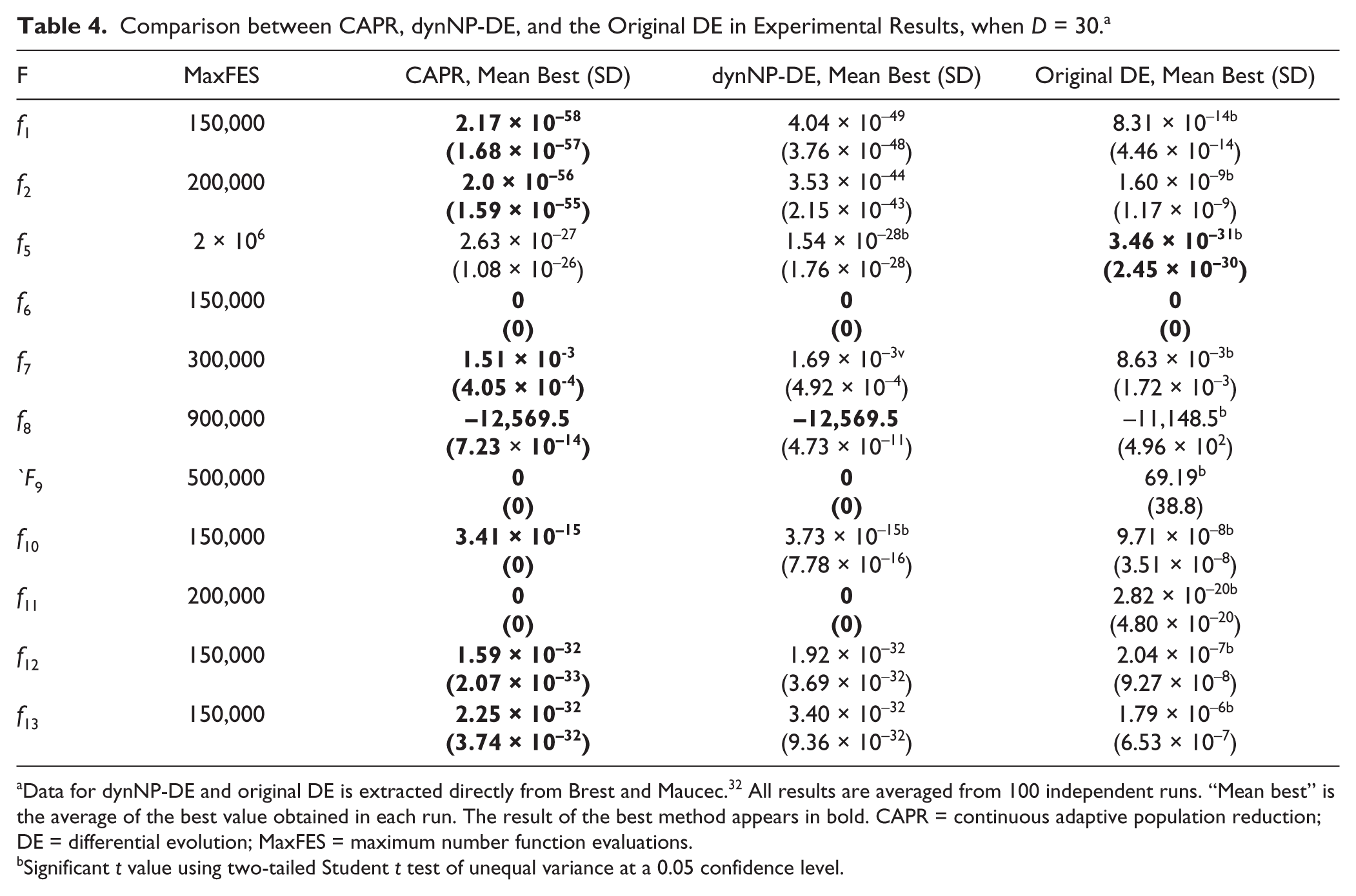
Data for dynNP-DE and original DE is extracted directly from Brest and Maucec.³² All results are averaged from 100 independent runs. “Mean best” is the average of the best value obtained in each run. The result of the best method appears in bold. CAPR = continuous adaptive population reduction; DE = differential evolution; MaxFES = maximum number function evaluations.

Significant t value using two-tailed Student t test of unequal variance at a 0.05 confidence level.

The optimal results from 100 independent runs of each function were averaged and are listed in Table 4 as “mean best.” For each function, the result of the best method is highlighted in bold. All mean best results between CAPR and other methods were statistically compared using a two-tailed Student t test of unequal variance with a confidence level of 0.05. As shown in Table 4 , CAPR presented better results for all functions compared with the dynNP-DE, except f₅. Functions f₁ and f₂ presented a couple orders of magnitude improvement over the dynNP-DE algorithm, and f₁₀ showed 0 standard deviations. For function f₅, both our algorithm and the dynNP-DE algorithm outperformed the original DE algorithm, most likely because of the population reduction, which decreases the diversity in the population. However, the results in Table 4 show that CAPR has the best overall performance compared with the dynNP-DE and original DE algorithm.

A parametric study of the CAPR method was investigated with different values of NP_init ∈ {200, 400} and α ∈ {10, 50, 100, 250, 500, 1000}. MaxFES remained the same as shown in Table 4 . The average of the best (mean best) and standard deviation of the average of the best, as well as the number of successful tests that did not get trapped in local optimum, are presented in Table 5 . Fitness value considered as trapped in local optimum is at least 10¹⁰ higher than the mean best value. For most functions with α = 10, the population size NP shrunk too fast and therefore easily got trapped in the local optimum. This can be seen from the fitness and population size plots ( Figs. 1 and 2 ). Therefore, α = 10 could be served as the lower bound in this algorithm and should always be avoided. For α = 50, the only challenging function is f₅, which got trapped in local optimum with a probability of about 3/100 and 10/100 for NP_init = 400 and 200, respectively. No trapping in local optimum was found for all functions when α ≥ 100 for NP_init ∈ {200, 400}. For α ∈ {500, 1000}, the results are not as good as the results of α ∈ {50, 100, 250}, mainly because the system has very slow population reduction, closely approaching the purely self-adaptive DE algorithm without population reduction. This could also be seen from the NP curves ( Figs. 1 and 2 ). For all tested functions, the best results can be found when α = 100 and NP_init = 200. We therefore use these settings for all studies in the later sections, unless otherwise stated.

Table 5.

Parametric Study of CAPR when D = 30.^a

F	NP_init	α = 10, Mean Best (SD)	α = 50, Mean Best (SD)	α = 100, Mean Best (SD)	α = 250, Mean Best (SD)	α = 500, Mean Best (SD)	α =1000, Mean Best (SD)
f ₁	200	9.99 × 10⁻⁹⁴ (4.90 × 10⁻⁹³) [100/100]	3.81 × 10⁻⁷⁹ 3.81 × 10⁻⁷⁸ [100/100]	2.17 × 10⁻⁵⁸ (1.68 × 10⁻⁵⁷) [100/100]	1.50 × 10⁻¹⁶ (3.36 × 10⁻¹⁶) [100/100]	1.47 × 10⁻¹² (1.08 × 10⁻¹²) [100/100]	5.28 × 10⁻¹² (2.54 × 10⁻¹²) [100/100]
f ₁	400	6.31 × 10⁻⁸⁸ (5.25 × 10⁻⁸⁷) [100/100]	1.47 × 10⁻⁶⁰ 1.32 × 10⁻⁵⁹ [100/100]	2.62 × 10⁻¹⁶ (1.56 × 10⁻¹⁵) [100/100]	4.31 × 10⁻⁵ (3.07 × 10⁻⁵) [100/100]	5.27 × 10⁻⁴ (1.61 × 10⁻⁴) [100/100]	9.80 × 10⁻⁴ (2.61 × 10⁻⁴) [100/100]
f ₂	200	4.13 × 10⁻⁷⁹ (2.26 × 10⁻⁷⁸) [100/100]	1.05 × 10⁻⁷² 8.61 × 10⁻⁷² [100/100]	2.0 × 10⁻⁵⁶ (1.59 × 10⁻⁵⁵) [100/100]	1.05 × 10⁻¹⁵ (6.21 × 10⁻¹⁵) [100/100]	7.83 × 10⁻¹² (5.77 × 10⁻¹²) [100/100]	5.98 × 10⁻¹¹ (2.54 × 10⁻¹¹) [100/100]
f ₂	400	3.40 × 10⁻⁷⁵ (1.20 × 10⁻⁷⁴) [100/100]	6.67 × 10⁻⁵¹ 6.67 × 10⁻⁵⁰ [100/100]	8.40 × 10⁻²⁶ (8.26 × 10⁻²⁵) [100/100]	2.95 × 10⁻⁶ (2.99 × 10⁻⁶) [100/100]	5.39 × 10⁻⁵ (2.17 × 10⁻⁵) [100/100]	1.28 × 10⁻⁴ (3.09 × 10⁻⁵) [100/100]
f ₅	200	2.66 × 10⁻²⁷ 8.40 × 10⁻²⁷ [70/100]	1.07 × 10⁻²⁷ (1.78 × 10⁻²⁷) [90/100]	2.63 × 10⁻²⁷ (1.08 × 10⁻²⁶) [100/100]	2.59 × 10⁻²⁸ (4.16 × 10⁻²⁸) [100/100]	4.95 × 10⁻²⁹ (5.11 × 10⁻²⁹) [100/100]	2.74 × 10⁻²⁹ (2.73 × 10⁻²⁹) [100/100]
f ₅	400	1.54 × 10⁻²⁷ 3.35 × 10⁻²⁷ [78/100]	2.94 × 10⁻²⁷ 1.01 × 10⁻²⁶ [97/100]	2.58 × 10⁻²⁷ (9.63 × 10⁻²⁷) [100/100]	2.30 × 10⁻²⁸ (3.56 × 10⁻²⁸) [100/100]	3.98 × 10⁻²⁹ (2.96 × 10⁻²⁹) [100/100]	4.92 × 10⁻¹⁴ (2.56 × 10⁻¹³) [100/100]
f ₆	200	0 (0) [100/100]	0 (0) [100/100]	0 (0) [100/100]	0 (0) [100/100]	0 (0) [100/100]	0 (0) [100/100]
f ₆	400	0 (0) [100/100]	0 (0) [100/100]	0 (0) [100/100]	0 (0) [100/100]	0 (0) [100/100]	0 (0) [100/100]
f ₇	200	1.77 × 10⁻³ (8.15 × 10⁻⁴) [100/100]	1.33 × 10⁻³ 3.95 × 10⁻³ [100/100]	1.51 × 10⁻³ (4.05 × 10⁻⁴) [100/100]	4.20 × 10⁻³ (9.52 × 10⁻⁴) [100/100]	5.74 × 10⁻³ (1.21 × 10⁻³) [100/100]	5.84 × 10⁻³ (1.22 × 10⁻³) [100/100]
f ₇	400	1.51 × 10⁻³ 5.77 × 10⁻⁴ [100/100]	1.43 × 10⁻³ 4.59 × 10⁻⁴ [100/100]	2.37 × 10⁻³ (6.97 × 10⁻³) [100/100]	8.34 × 10⁻³ (1.90 × 10⁻³) [100/100]	1.08 × 10⁻² (2.41 × 10⁻³) [100/100]	1.12 × 10⁻² (2.40 × 10⁻³) [100/100]
f ₈	200	−12,430.8 (1.47 × 10²) [100/100]	−12,568.3 1.18 × 10¹ [100/100]	−12,569.5 (7.23 × 10⁻¹⁴) [100/100]	−12,569.5 (1.54 × 10⁻¹³) [100/100]	−12,569.5 (2.58 × 10⁻¹³) [100/100]	−12,569.5 (3.04 × 10⁻¹³) [100/100]
f ₈	400	−12,492.8 1.04 × 10² [100/100]	−12,569.5 6.96 × 10⁻¹⁴ [100/100]	−12,569.5 (7.77 × 10⁻¹⁴) [100/100]	−12,569.5 (2.20 × 10⁻¹³) [100/100]	−12,569.5 (4.46 × 10⁻¹³) [100/100]	−12,569.5 (5.68 × 10⁻¹³) [100/100]
f ₉	200	0 (0) [91/100]	0 (0) [100/100]	0 (0) [100/100]	0 (0) [100/100]	0 (0) [100/100]	0 (0) [100/100]
f ₉	400	0 (0) [100/100]	0 (0) [100/100]	0 (0) [100/100]	0 (0) [100/100]	3.53 × 10⁻¹⁵ (1.00 × 10⁻¹⁴) [100/100]	5.95 × 10⁻¹¹ (8.49 × 10⁻¹¹) [100/100]
f ₁₀	200	3.41 × 10⁻¹⁵ (0) [99/100]	3.41 × 10⁻¹⁵ (0) [100/100]	3.41 × 10⁻¹⁵ (0) [100/100]	5.27 × 10⁻⁹ (5.01 × 10⁻⁹) [100/100]	4.50 × 10⁻⁷ (1.86 × 10⁻⁷) [100/100]	8.64 × 10⁻⁷ (2.97 × 10⁻⁷) [100/100]
f ₁₀	400	3.41 × 10⁻¹⁵ (0) [100/100]	3.41 × 10⁻¹⁵ (0) [100/100]	9.76 × 10⁻⁹ (7.29 × 10⁻⁸) [100/100]	4.00 × 10⁻³ (2.34 × 10⁻⁴) [100/100]	8.54 × 10⁻³ (1.73 × 10⁻³) [100/100]	1.23 × 10⁻² (2.30 × 10⁻³) [100/100]
f ₁₁	200	0 (0) [83/100]	0 (0) [100/100]	0 (0) [100/100]	0 (0) [100/100]	7.37 × 10⁻²⁰ (8.56 × 10⁻²⁰) [100/100]	2.58 × 10⁻¹⁷ (4.78 × 10⁻¹⁶) [100/100]
	400	0(0)[78/100]	0(0)[100/100]	0(0)[100/100]	1.38 × 10⁻⁸ (2.08 × 10⁻⁸)[100/100]	1.86 × 10⁻⁶ (2.92 × 10⁻⁶)[100/100]	6.27 × 10⁻⁶ (3.55 × 10⁻⁶)[100/100]
f ₁₂	200	1.60 × 10⁻³² (2.18 × 10⁻³³)[95/100]	1.59 × 10⁻³² (8.85 × 10⁻³⁴)[100/100]	1.59 × 10⁻³² (2.07 × 10⁻³³)[100/100]	2.41 × 10⁻¹⁸ (8.13 × 10⁻¹⁸)[100/100]	3.08 × 10⁻¹⁴ (2.98 × 10⁻¹⁴)[100/100]	2.61 × 10⁻¹³ (1.56 × 10⁻¹³)[100/100]
f ₁₂	400	2.30 × 10⁻³² 3.80 × 10⁻³² [99/100]	2.18 × 10⁻³² (6.03 × 10⁻³²)[100/100]	4.43 × 10⁻¹⁶ (4.38 × 10⁻¹⁵)[100/100]	7.41 × 10⁻⁷ (8.79 × 10⁻⁷)[100/100]	1.56 × 10⁻⁵ (7.00 × 10⁻⁶)[100/100]	4.44 × 10⁻⁵ (1.59 × 10⁻⁵)[100/100]
f ₁₃	200	3.07 × 10⁻³² (1.03 × 10⁻³¹)[93/100]	2.27 × 10⁻³² (3.73 × 10⁻³³)[100/100]	2.25 × 10⁻³² (3.74 × 10⁻³²)[100/100]	4.18 × 10⁻¹⁷ (1.27 × 10⁻¹⁶)[100/100]	4.25 × 10⁻¹³ (4.07 × 10⁻¹³)[100/100]	3.00 × 10⁻¹² (1.94 × 10⁻¹²)[100/100]
	400	2.30 × 10⁻³² (3.80 × 10⁻³²)[98/100]	2.89 × 10⁻³² (1.05 × 10⁻³¹)[100/100]	7.63 × 10⁻¹⁹ (6.66 × 10⁻¹⁸)[100/100]	7.09 × 10⁻⁶ (4.99 × 10⁻⁶)[100/100]	1.54 × 10⁻⁴ (7.21 × 10⁻⁵)[100/100]	4.10 × 10⁻⁴ (1.19 × 10⁻⁴)[100/100]

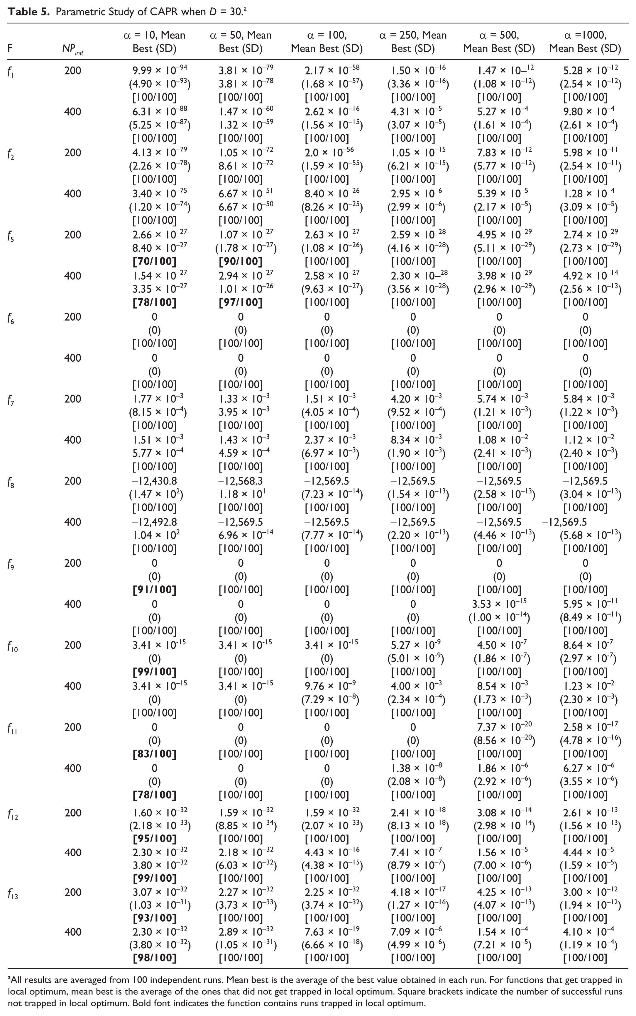
All results are averaged from 100 independent runs. Mean best is the average of the best value obtained in each run. For functions that get trapped in local optimum, mean best is the average of the ones that did not get trapped in local optimum. Square brackets indicate the number of successful runs not trapped in local optimum. Bold font indicates the function contains runs trapped in local optimum.

Significant improvements in convergence speed can be seen when dimension D is increased to 60 and 90 ( Table 6 ; Fig. 3 ). Comparing this to the results of dynNP-DE, the overall average numbers of function evaluations (FES) needed for CAPR to reach VTR are significantly lower than those needed by dynNP-DE. At D = 60, we tested two initial population sizes, NP_init ∈ {200, 400} for both CAPR and dynNP-DE. For dynNP-DE, pmax = 4 is used when NP_init = 200 and pmax = 5 is used when NP_init = 400. These are the experimental conditions recommended by Brest and Maucec.³² Other control parameter settings remain unchanged, as in the experiments in Table 4 , except for MaxFES, which is doubled. At both NP_init values, CAPR showed significant convergence speed improvement for all functions. When NP_init = 200, CAPR can reach VTR in less than half of the FES needed by dynNP-DE for f₂, f₅, and f₇ to f₁₁. Similar results are found when NP_init = 400, where CAPR needs less than half of the FES of dynNP-DE to reach VTR for f₂, f₅, f₈, and f₉. From Table 6 , it seems that for both methods, a lower initial population size would lead to a faster convergence, but it should be noted that a low population sometimes could lead to a local optimum trap. Similar to dynNP-DE, f₅ is still found to be a challenging function that may be trapped in local optima. When D is increased to 90, similar improvement is found. Here, pmax = 5 is used for dynNP-DE. CAPR is found to require less than half of what is needed for dynNP-DE to reach VTR for f₂ and f₇ to f₁₀ and less than one-third of what is needed for dynNP-DE to reach VTR for f₈ and f₉.

Table 6.

Comparison between CAPR, dynNP-DE, and Original DE in Average FES to Reach VTR when D = 60 and 90.^a

			D = 60		D = 60		D = 90
			NP_init = 200		NP_init = 400		NP_init = 400
F	MaxFES	VTR	CAPR, Mean FES (SD)	dynNP-DE, Mean FES (SD)	CAPR, Mean FES (SD)	dynNP-DE, Mean FES (SD)	CAPR, Mean FES (SD)	dynNP-DE, Mean FES (SD)
f ₁	300,000	1 × 10⁻¹²	91,780(4612.6)	157,387^b (1150.5)	143,851(7739.5)	191,778^b ⁽1232.5)	168,863(7400.4)	212,977^b ⁽4176.5)
f ₂	400,000	1 × 10⁻¹²	91,354(8137.6)	218,719^b ⁽1384.3)	135,772(15,619)	264,514^b (1500.8)	156,343(14,764.4)	291,406^b ₍3954.7)
f ₅	6 × 10⁶	1 × 10⁻¹²	1.23 × 10^6c (167,215)	2.26 × 10^6b,d (48,153.7)	1.27 × 10^6e (168,911)	2.80 × 10^6b (27,746.6)	3.70 × 10^6f (520,330)	3,84 × 10^6b (58,566.5)
f ₆	300,000	1 × 10⁻¹²	47,120(2300.1)	75,235^b (1635.9)	89,033(4611.7)	107,948^b (1952.2)	100,551(5648.5)	125,696^b (2001.3)
f ₇	600,000	1 × 10⁻²	163,845(25,850.5)	348,026^b (40,686.8)	234,762(26,478.6)	429,269^b ⁽43,613.5)	279,905(35,901.7)	502,409^b,g (40,535.3)
f ₈	1.8 × 10⁶	−25,139^h	127,364(8225.7)	320,412^b (6094.6)	209,127(16,428.7)	552,395^b (11,712.7)	244,323(16,833.8)	750,960^b (20,408.8)
f ₉	1 × 10⁶	1 × 10¹	117,494(9906.9)	272,590^b (7264.0)	197,288(14,756.3)	455,794^b (15,229.3)	222,745(14,634.7)	611,184^b (31,733.1)
f ₁₀	300,000	1 × 10⁻⁹	111,646(5980.6)	213,373^b (26,570.2)	168,362(8467.1)	255,179^b (18,937.9)	219,677(14,584.2)	N/Aⁱ (N/A)
f ₁₁	400,000	1 × 10⁻¹²	91,747(5316.6)	176,377^b (2082.5)	145,475(7382.8)	227,607^b (1891.6)	168,316(9340.05)	250,117^b (2907.8)
f ₁₂	300,000	1 × 10⁻¹²	93,494(5566.8)	153,819^b (1290.6)	152,289(9901.43)	189,603^b (1229.26)	181,614(10,113)	209,518^b (3097.6)
f ₁₃	300,000	1 × 10⁻¹²	96,653(4868.4)	157,698^b (1115.9)	156,082(9669.62)	192,889^b ⁽1240.9)	185,197(10,533)	214,764^b (3544.4)

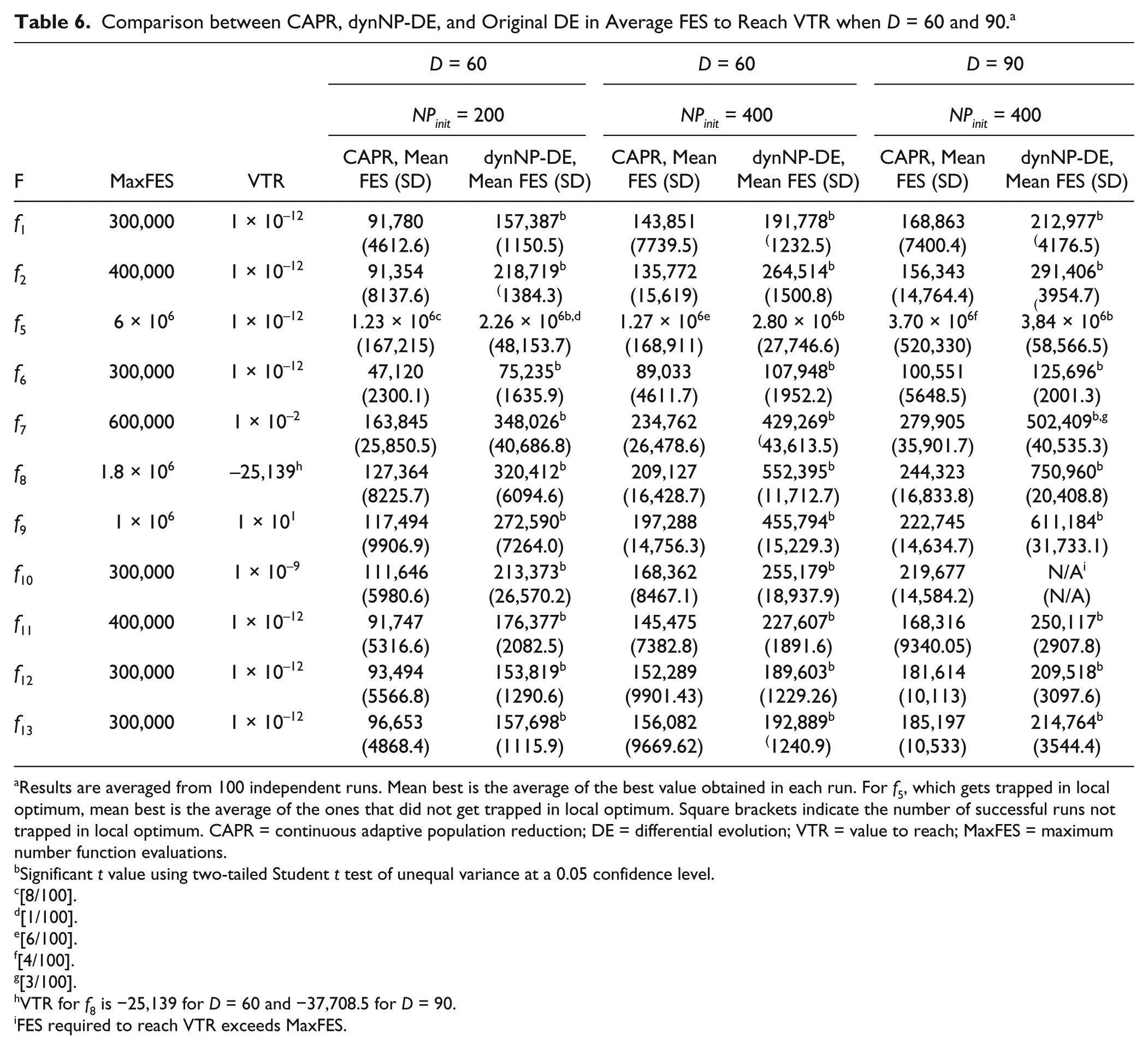
Results are averaged from 100 independent runs. Mean best is the average of the best value obtained in each run. For f₅, which gets trapped in local optimum, mean best is the average of the ones that did not get trapped in local optimum. Square brackets indicate the number of successful runs not trapped in local optimum. CAPR = continuous adaptive population reduction; DE = differential evolution; VTR = value to reach; MaxFES = maximum number function evaluations.

Significant t value using two-tailed Student t test of unequal variance at a 0.05 confidence level.

[8/100].

[1/100].

[6/100].

[4/100].

[3/100].

VTR for f₈ is −25,139 for D = 60 and −37,708.5 for D = 90.

FES required to reach VTR exceeds MaxFES.

Figure 3.

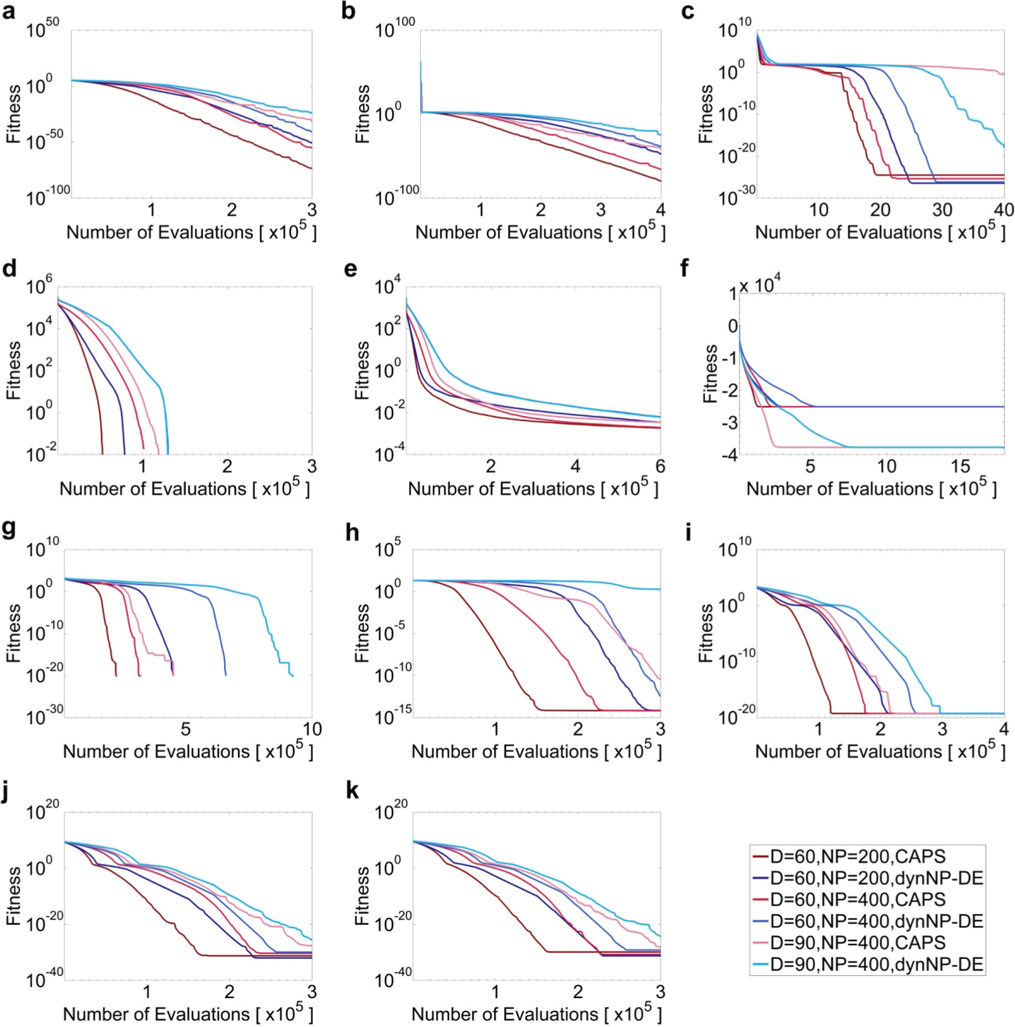
Comparison of average fitness values of all performing agents averaged over 100 independent experiments for f₁ (a), f₂ (b), f₅ (c), f₆ (d), f₇ (e), f₈ (f), f₉ (g), f₁₀ (h), f₁₁ (i), f₁₂ (j), and f₁₃ (k) between CAPR (red color–based lines) and dynNP-DE algorithms (blue color–based lines; see legends).

Graphs plotted in Figures 1 and 2 show the fitness and population size evolutionary dynamics for the benchmark functions f₁ to f₁₃ under various values of α at a dimension of D = 30. All settings remain unchanged as the experiments in Table 4 . Both the curves of average fitness and NP values were plotted. The graphs illustrate clearly the dependence of the optimization process on the values of α. The averaged curves did not involve the ones that get trapped in local optimum, which happened only for α = 10 and a few for α = 50 (see bolded fonts in Table 5 ). This is because local optima usually have values of at least 10¹⁰ higher than the average value and will therefore greatly affect the trend of the curves. For α = 10, NP values dropped to NP_min too fast for most functions (within 1/10th of the MaxFES), and therefore, the final results may be easily trapped into local optimum. For most functions, except f₅, α = 500 and 1000 shows very similar fitness value dynamics and therefore can be considered as a saturation value of α for most functions. Moreover, when α = 1000, NP stays almost unchanged throughout the whole evolutionary process for all functions, except f₅. This is very close to the self-adaptive DE algorithm (jDE) without population reduction.²⁷ This could also be seen from the parametric study shown in Table 5 . Nonetheless, the graphs present a robust performance and improved convergence efficiency of CAPR.

Figure 3 presents the comparison between CAPR and dynNP-DE on the iteration dynamics of the average fitness and NP values at D = 60 and 90 with NP_init ∈ {200, 400}. Both the curves of best fitness and NP values are plotted. Same as Table 6 and Figure 3 , pmax = 4 is used for NP_init = 200 and pmax = 5 is used for NP_init = 400 for the dynNP-DE algorithm. The other control parameter settings remain unchanged as the previous experiments. For all functions, CAPR reaches optimal fitness faster than dynNP-DE when comparing to figs. 15 to 25 in Brest and Maucec.³¹

We also tested some low-dimensional functions, f₁₄ to f₂₁, which have only a few local minima.⁵⁴ Because the dimension D is much lower than the previous experiments, we lowered NP_init to 50 as suggested previously, where NP_init should be chosen to be about 5 × D to 10 × D². Moreover, NP_min is also lowered to 4. Table 7 shows the comparison of performance of CAPR with dynNP-DE and the original DE.

Table 7.

Comparison between CAPR, dynNP-DE, and Original DE in Experimental Results, when D = 30.^a.

F	MaxFES	CAPR, Mean FES (SD)	dynNP-DE, Mean FES (SD)	Original DE, Mean FES (SD)
f ₁₄	10,000	0.998004 (1.89 × 10⁻¹⁷)	0.998004 (8.04 × 10⁻¹⁸)	0.998004 (2.13 × 10⁻¹⁵)
f ₁₅	400,000	3.90 × 10⁻⁴ (2.63 × 10⁻⁴)	3.34 × 10⁻⁴ (1.57 × 10⁻⁴)	4.35 × 10⁻⁴ (3.19 × 10⁻⁴)
f ₁₆	10,000	–1.03163 (6.60 × 10⁻¹⁷)	–1.03163 (1.34 × 10⁻¹⁵)	–1.03163 (4.95 × 10⁻¹³)
f ₁₇	10,000	0.397887 (0)	0.397887 (1.06 × 10⁻¹⁵)	0.397887 (7.20 × 10⁻⁹)
f ₁₈	10,000	3 (7.85 × 10⁻¹⁸)	3 (1.20 × 10⁻¹⁵)	3 (0)
f ₁₉	10,000	–10.1532 (5.94 × 10⁻¹⁵)	–10.1532 (9.72 × 10⁻¹³)	–10.1532 (1.29 × 10⁻⁵)
f ₂₀	10,000	–10.4029 (7.35 × 10⁻¹⁶)	–10.4029 (2.21 × 10⁻¹⁵)	−10.4029 (6.12 × 10⁻⁷)
f ₂₁	10,000	–10.5364 (6.02 × 10⁻¹⁶)	–10.5364 (1.56 × 10⁻¹⁵)	–10.5364 (2.18 × 10⁻⁷)

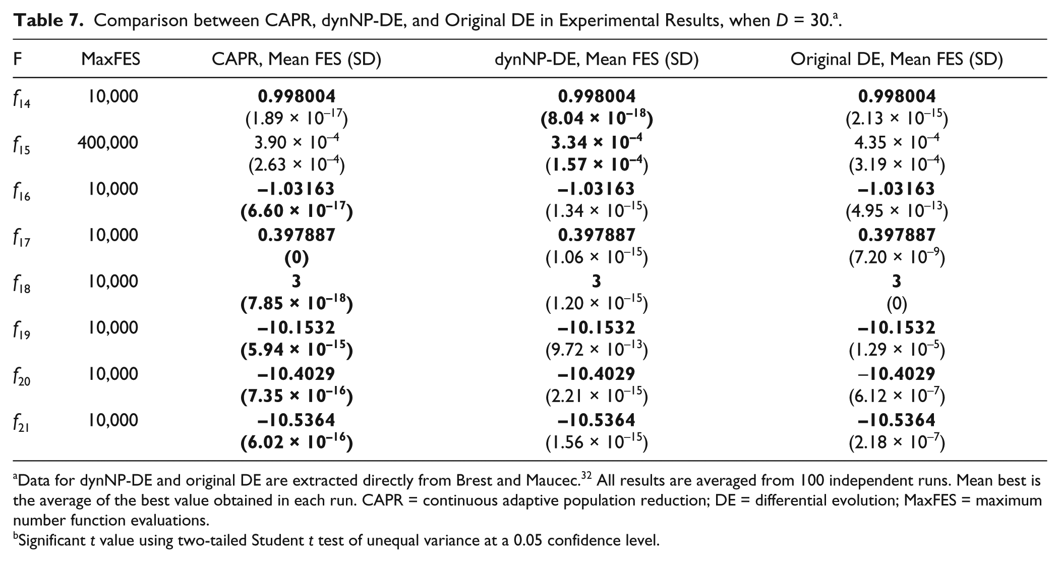
Data for dynNP-DE and original DE are extracted directly from Brest and Maucec.³² All results are averaged from 100 independent runs. Mean best is the average of the best value obtained in each run. CAPR = continuous adaptive population reduction; DE = differential evolution; MaxFES = maximum number function evaluations.

Significant t value using two-tailed Student t test of unequal variance at a 0.05 confidence level.

CAPR shows slightly better performance than dynNP-DE for most functions, except f₁₄ and f₁₅. Other than f₁₅, all three methods can reach the same global optimal values with CAPR showing the best in terms of standard deviations. Considering the fact that even the original DE can reach the global optimal values, which is not the case for f₁ to f₁₃, it is hard to realize the full capacity of CAPR because of the simplicity of these low-dimensional functions.

Moreover, we performed a characterization of the population truncation methods during the population reduction process. One is by random truncation, which eliminates the excessive number of agents randomly, and this is the scheme we have been using in all of the previous experiments. The other one is through a sorted truncation, which eliminates the excessive number of the poorest-performing agents from the population. Parameter settings are the same as those in the experiments shown in Table 4 and Table 7 , where NP_init = 200 and α = 100. As shown in Table 8 , the random truncation scheme results in relatively better convergence than the random truncation scheme for most functions, except f₁, f₂, and f₇. This is most likely because keeping a more diverse population could prevent the optimization process from getting trapped in local optima, thus enhancing exploration.

Table 8.

Comparison of Experimental Results between Random Truncation and Sorted Truncation for CAPR and dynNP-DE at D = 30.^a.

		CAPR		dynNP-DE
F	MaxFES	Unsorted, Mean Best (SD)	Sorted, Mean Best (SD)	Mean Best, (SD)
f ₁	150,000	2.17 × 10⁻⁵⁸ (1.68 × 10⁻⁵⁷)	6.06 × 10⁻⁵⁹ (5.94 × 10⁻⁵⁸)	4.04 × 10⁻⁴⁹ (3.76 × 10⁻⁴⁸)
f ₂	200,000	2.0 × 10⁻⁵⁶ ⁽1.59 × 10⁻⁵⁵)	4.79 × 10⁻⁵⁹ (3.59 × 10⁻⁵⁸)	3.53 × 10⁻⁴⁴ (2.15 × 10⁻⁴³)
f ₅	2 × 10⁶	2.63 × 10^−27b (1.08 × 10⁻²⁶)	1.70 × 10^{−27b[5/100]} (4.09 × 10⁻²⁷)	1.54 × 10⁻²⁸ (1.76 × 10⁻²⁸)
f ₆	150,000	0 (0)	11.02^b (5.07)	0 (0)
f ₇	300,000	1.51 × 10^−3b (4.05 × 10⁻⁴)	1.15 × 10⁻³^b (3.69 × 10⁻⁴)	1.69 × 10⁻³ (4.92 × 10⁻⁴)
f ₈	900,000	–12,569.5 (7.23 × 10⁻¹⁴)	−12,569.5(1.99 × 10⁻¹³)	–12,569.5 (4.73 × 10⁻¹¹)
f ₉	500,000	0 (0)	0.63 × 10⁻²⁷ (1.08 × 10⁻²⁶)	0 (0)
f ₁₀	150,000	3.41 × 10⁻¹⁵^b (0)	2.75 × 10^−13b (2.53 × 10⁻¹³)	3.73 × 10⁻¹⁵ (7.78 × 10⁻¹⁶)
f ₁₁	200,000	0 (0)	5.01 × 10^−19b (1.49 × 10⁻¹⁹)	0 (0)
f ₁₂	150,000	1.59 × 10⁻³² (2.07 × 10⁻³³)	2.73 × 10⁻³² (2.62 × 10⁻³²)	1.92 × 10⁻³² (3.69 × 10⁻³²)
f ₁₃	150,000	2.25 × 10⁻³² (3.74 × 10⁻³²)	4.57 × 10⁻³² (6.25 × 10⁻³²)	3.40 × 10⁻³² (9.36 × 10⁻³²)
f ₁₄	10,000	0.998004 (1.89 × 10⁻¹⁷)	0.998004 (8.04 × 10⁻⁷)	0.998004 (8.04 × 10⁻¹⁸)
f ₁₅	400,000	3.90 × 10⁻⁴ (2.63 × 10⁻⁴)	3.53 × 10⁻⁴ (2.01 × 10⁻⁴)	3.34 × 10⁻⁴ (1.57 × 10⁻⁴)
f ₁₆	10,000	–1.03163 (6.60 × 10⁻¹⁷)	–1.03163 (3.35 × 10⁻⁷)	–1.03163 (1.34 × 10⁻¹⁵)
f ₁₇	10,000	0.397887 (0)	0.397891^b (9.17 × 10⁻⁶)	0.397887 (1.06 × 10⁻¹⁵)
f ₁₈	10,000	3 (7.85 × 10⁻¹⁸)	3 (2.36 × 10⁻⁹)	3 (1.20 × 10⁻¹⁵)
f ₁₉	10,000	–10.1532 (5.94 × 10⁻¹⁵)	−9.7148^b (5.17 × 10⁻¹)	–10.1532 (9.72 × 10⁻¹³)
f ₂₀	10,000	–10.4029 (7.35 × 10⁻¹⁶)	−10.3441^b (7.59 × 10⁻²)	–10.4029 (2.21 × 10⁻¹⁵)
f ₂₁	10,000	–10.5364 (6.02 × 10⁻¹⁶)	−10.4692 ^† (9.87 × 10⁻²)	–10.5364 (1.56 × 10⁻¹⁵)

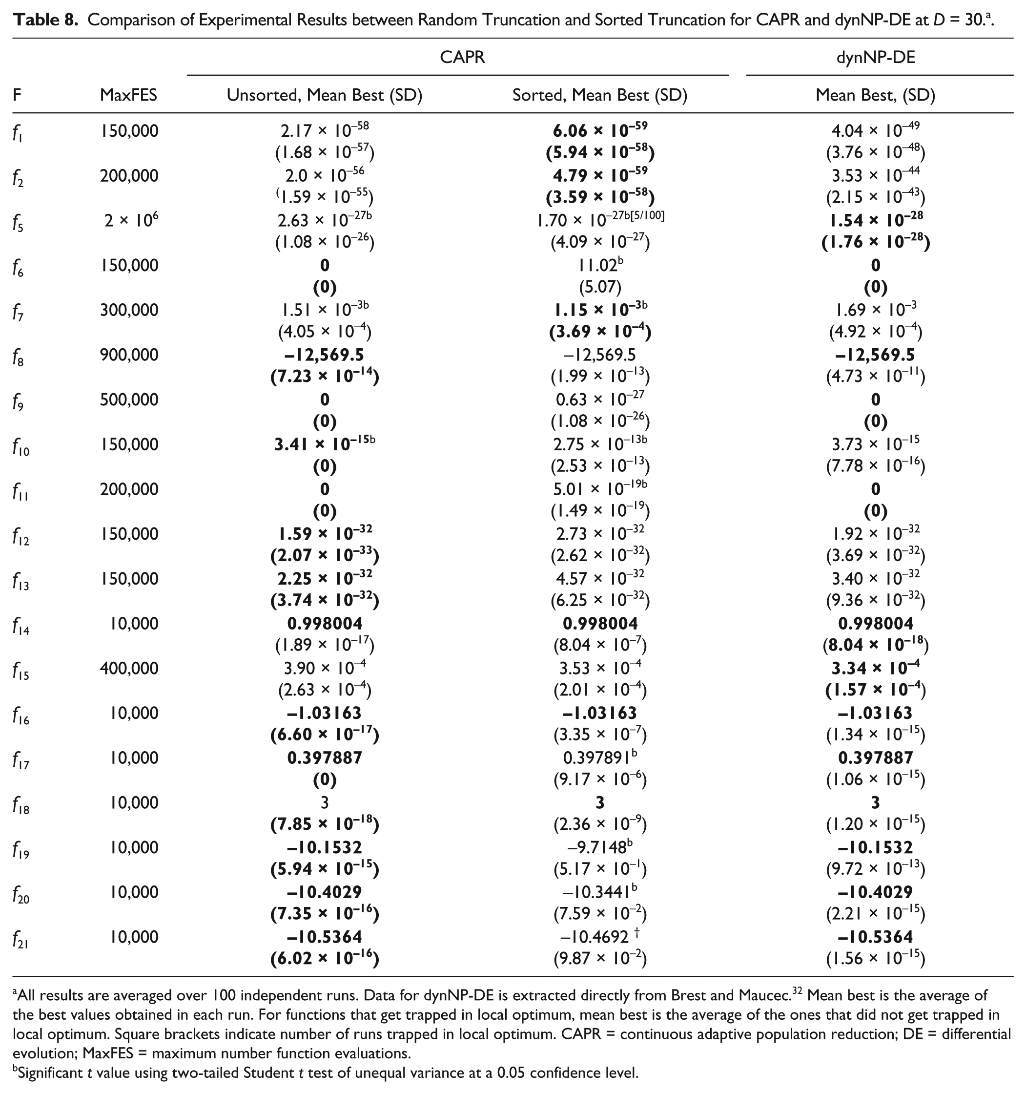
All results are averaged over 100 independent runs. Data for dynNP-DE is extracted directly from Brest and Maucec.³² Mean best is the average of the best values obtained in each run. For functions that get trapped in local optimum, mean best is the average of the ones that did not get trapped in local optimum. Square brackets indicate number of runs trapped in local optimum. CAPR = continuous adaptive population reduction; DE = differential evolution; MaxFES = maximum number function evaluations.

Significant t value using two-tailed Student t test of unequal variance at a 0.05 confidence level.

Discussion

As inspired by the dynamic population reduction scheme (dynNP-DE), our proposed dynamic population reduction algorithm is designed to interact dynamically with the optimization space to more effectively distribute the population. Our population reduction scheme works by distributing the number of populations in response to the average fitness value in a continuous fashion, in contrast to a stepwise population reduction scheme of dynNP-DE. The study shows that updating the population size adaptively to the exploration-exploitation stage in the evolutionary process is an effective way to enhance the DE convergence efficiency.

One important feature of our population reduction scheme is that we limit the population reduction to happen only when the gradient ratio (Δ_G/Δ_G-1) is between 0 and 1. This limits exploitation (refining the best population) to occur only when improvement starts to slow down. If the gradient ratio of the current iteration is greater than 1 (much better performance than previous iteration) or worse than that in the previous generation, no population reduction will take place.

It is always desirable to have an optimization algorithm be both effective and robust. CAPR improves, besides the final fitness values, significantly on the speed of convergence. Such improvements are significant when the dimension is D = 60 and 90, where the average number of FES required for CAPR to reach the predefined VTR can be as low as half of those needed by dynNP-DE.

According to our parametric study, we found that a higher initial population may not always be helpful to the optimization problem. As shown in Table 5 , a higher NP_init is helpful only when the population reduction is too fast (when α = 10) by lowering the chance of being trapped in local optimum. However, when population reduction is slower (α ≥ 50), all functions perform better when NP_init is indeed smaller, except f₅. We believe that the performance of a DE algorithm truly relies on the proper balance between exploration (requires a diverse population) and exploitation (requires a refined population). A similar situation is also found on selecting α, which controls the population reduction rate. At the two extremes, α = 10 and 1000, DE either reduces the population too fast or reduces the population too slow, which greatly affects the final results. Similar observations have recently been discussed by Neri and Tirronen.⁵ This observation is in contrast to the common consensus that population-based evolutionary algorithms always desire a large pool of diverse population at the beginning. Although. currently, we do not have a self-adaptive mechanism of providing the optimal balance for all functions, this study proposed some best-parameter settings for CAPR, which could yield better overall results for most functions: NP_init = 200 and α = 100 for D ∈ {30, 60}.

One important process that surprises us is the agent elimination step during population reduction. The random truncation method is relatively better than the sorted truncation method. The random truncation method prevents the algorithm from always picking the best individuals during the evolution, which may trap the optimization into local optimum. Random truncation also does not need any extra sorting process, which will increase the time complexity compared with the unsorted truncation method.

Conclusions

This article proposes a population reduction mechanism for the DE algorithm, namely, CAPR. The performance of the method is evaluated through the use of a number of unimodal and multimodal benchmark functions. The new method improved the convergence speed compared with the stepwise population dynNP-DE scheme. We believe the improvement is due to the fact that our population reduction scheme is continuously responding to the progression of the optimization process, which more effectively and adaptively controls the population size during the evolutionary process, in accordance with the exploration and exploitation stages.

The article also presents parametric analysis on the control parameters involved in the continuous population reduction scheme, namely, α and NP_init, which control the population reduction rate in response to the optimization progress and the initial population size, respectively. The plotted curves of the fitness and NP values illustrate the evolutionary dynamics of CAPR and provide us information on the boundaries on the choice of these control parameters. Because the method does not require any additional sorting or comparison of the agents in the population, no additional cost is introduced, except the calculation for a new NP value after one cycle of evaluations of all agents.

An extension of our population reduction method is to include the population increment method to further improve DE. Furthermore, because there is still much less work available on the self-adaptive population control method in contrast to the self-adaptive F and CR control method, future investigations into a completely parameter tune-free self-adaptive DE algorithm will be greatly beneficial.

Footnotes

Declaration of Conflicting Interests

The authors declared no potential conflicts of interest with respect to the research, authorship, and/or publication of this article.

Funding

The authors disclosed receipt of the following financial support for the research, authorship, and/or publication of this article: This work was supported by National Natural Science Foundation of China (81301293) and National Science and Technology Major Projects for “Major New Drugs Innovation and Development” (2014ZX09507008).

References

Price

Storn

R. M.

Lampinen

J. A.

Differential Evolution: A Practical Approach to Global Optimization; Springer Science & Business Media: Berlin, 2006.

Storn

Price

Differential Evolution—A Simple and Efficient Heuristic for Global Optimization over Continuous Spaces. J. Glob. Optim. 1997, 11, 341–359.

Tang

Dong

Liu

Differential Evolution with an Individual-Dependent Mechanism. Evol. Comput. IEEE Trans. 2015, 19, 560–574.

Biswas

Kundu

Das

An Improved Parent-Centric Mutation with Normalized Neighborhoods for Inducing Niching Behavior in Differential Evolution. IEEE Trans. Cybern. 2014, 44, 1726–1737.

Neri

Tirronen

Recent Advances in Differential Evolution: A Survey and Experimental Analysis. Artif. Intell. Rev. 2010, 33, 61–106.

Das

Suganthan

P. N.

Differential Evolution: A Survey of the State-of-the-Art. IEEE Trans. Evol. Comput. 2011, 15, 27–54.

Zhan

Situ

Yeung

L. F.

. A Parameter Estimation Method for Biological Systems Modelled by Ode/dde Models Using Spline Approximation and Differential Evolution Algorithm. IEEE/ACM Trans. Comput. Biol. Bioinforma. 2014, 11, 1066–1076.

Silva

Lee

B.-Y.

Clemens

D. L.

. Output-Driven Feedback System Control Platform Optimizes Combinatorial Therapy of Tuberculosis Using a Macrophage Cell Culture Model. Proc. Natl. Acad. Sci. U.S.A. 2016, 201600812.

Xiang

Meng

. An Enhanced Differential Evolution Algorithm Based on Multiple Mutation Strategies. Comput. Intell. Neurosci. 2015, 2015, 2.

10.

Zarrinpar

Lee

D.-K.

Silva

. Individualizing Liver Transplant Immunosuppression Using a Phenotypic Personalized Medicine Platform. Sci. Transl. Med. 2016, 8, 333ra49–333ra49.

11.

Rashid

M. B. M. A.

Toh

T. B.

Silva

. Identification and Optimization of Combinatorial Glucose Metabolism Inhibitors in Hepatocellular Carcinomas. J. Lab. Autom. 2015, 20, 423–437.

12.

Wang

Lee

D.-K.

Chen

K.-Y.

. Mechanism-Independent Optimization of Combinatorial Nanodiamond and Unmodified Drug Delivery Using a Phenotypically Driven Platform Technology. ACS Nano 2015, 9, 3332–3344.

13.

Ding

Drug Screening: Drug Repositioning Needs a Rethink. Nature 2016, 535, 355.

14.

Ding

Liu

Weiss

. Discovery of a Low Order Drug-Cell Response Surface for Applications in Personalized Medicine. Phys. Biol. 2014, 11, 65003.

15.

Ding

Sanchez

D. J.

Shahangian

. Cascade Search for HSV-1 Combinatorial Drugs with High Antiviral Efficacy and Low Toxicity. Int. J. Nanomed. 2012, 7, 2281–2292.

16.

Nowak-Sliwinska

Weiss

Ding

. Optimization of Drug Combinations Using Feedback System Control. Nat. Protoc. 2016, 11, 302–315.

17.

Tsutsui

Valamehr

Hindoyan

. An Optimized Small Molecule Inhibitor Cocktail Supports Long-Term Maintenance of Human Embryonic Stem Cells. Nat. Commun. 2011, 2, 167.

18.

Honda

Ding

Mussano

. Guiding the Osteogenic Fate of Mouse and Human Mesenchymal Stem Cells through Feedback System Control. Sci. Rep. 2013, 3, 3420.

19.

Feoktistov

Differential Evolution: In Search of Solutions (Springer Optimization and Its Applications); Springer-Verlag: New York, 2006.

20.

Storn

Differential Evolution Design of an IIR-Filter. Proc. IEEE Int. Conf. Evol. Comput. 1996, 268–273.

21.

Kim

H.-K.

Chong

J.-K.

Park

K.-Y.

. Differential Evolution Strategy for Constrained Global Optimization and Application to Practical Engineering Problems. IEEE Trans. Magn. 2007, 43, 1565–1568.

22.

Hachicha

Jarboui

Siarry

A Fuzzy Logic Control Using a Differential Evolution Algorithm Aimed at Modelling the Financial Market Dynamics. Inf. Sci. (Ny). 2011, 181, 79–91.

23.

Maciel

Gomide

Ballini

Modeling the Term Structure of Government Bond Yields with a Differential Evolution Algorithm. In Proceedings of the IEEE Conference on Computational Intelligence for Financial Engineering & Economics (CIFEr); IEEE Xplore: New York City, NY, USA, 2012; pp 1–8.

24.

Neri

Tirronen

Karkkainen

. Fitness Diversity Based Adaptation in Multimeme algorithms:A Comparative Study. In Proceedings of the IEEE Congress on Evolutionary Computation; IEEE Xplore: Singapore, 2007; Vol. 4, pp. 2374–2381.

25.

Plagianakos

V. P.

Tasoulis

D. K.

Vrahatis

M. N.

A Review of Major Application Areas of Differential Evolution. In Advances in Differential Evolution; Chakraborty

Ed.; Springer: Berlin Heidelberg, 2008; Vol. 143, pp 197–238.

26.

Ali

M. M.

Torn

Population Set-Based Global Optimization Algorithms: Some Modifications and Numerical Studies. Comput. Oper. Res. 2004, 31, 1703–1725.

27.

Brest

Greiner

Boskovic

. Self-Adapting Control Parameters in Differential Evolution: A Comparative Study on Numerical Benchmark Problems. IEEE Trans. Evol. Comput. 2006, 10, 646–657.

28.

Das

Konar

Chakraborty

U. K.

Two Improved Differential Evolution Schemes for Faster Global Search. In Proceedings of the Genetic and Evolutionary Computation Conference; ACM: Washington, DC, 2005; pp 991–998.

29.

Qin

A. K.

Suganthan

P. N.

Self-Adaptive Differential Evolution Algorithm for Numerical Optimization. In Proceed-ings of the IEEE Congress on Evolutionary Computation; IEEE Xplore: Edinburgh, UK, 2005; Vol. 2, pp 1785–1791.

30.

Yang

Cai

. Differential Evolution with Auto-Enhanced Population Diversity. IEEE Trans. Cybern. 2015, 45, 302–315.

31.

Brest

Maucec

M. S.

Population Size Reduction for the Differential Evolution Algorithm. Appl. Intell. 2008, 29, 228–247.

32.

Brest

Maucec

M. S.

Self-Adaptive Differential Evolution Algorithm Using Population Size Reduction and Three Strategies. Soft Comput. 2011, 15, 2157–2174.

33.

Liu

Lampinen

A Fuzzy Adaptive Differential Evolution Algorithm. Soft Comput. 2005, 9, 448–462.

34.

Teo

Exploring Dynamic Self-Adaptive Populations in Differential Evolution. Soft Comput. 2006, 10, 673–686.

35.

Neri

Tirronen

Scale Factor Local Search in Differential Evolution. Memetic Comput. 2009, 1, 153–171.

36.

Das

Abraham

Chakraborty

U. K.

. Differential Evolution Using a Neighborhood-Based Mutation Operator. IEEE Trans. Evol. Comput. 2009, 13, 526–553.

37.

Fan

H.-Y.

Lampinen

A Trigonometric Mutation Operation to Differential Evolution. J. Glob. Optim. 2003, 27, 105–129.

38.

Rahnamayan

Tizhoosh

H. R.

Salama

M. M. A.

Opposition-Based Differential Evolution. IEEE Trans. Evol. Comput. 2008, 12, 64–79.

39.

Mezura-Montes

Velazquez-Reyes

Coello Coello

C. A.

A Comparative Study of Differential Evolution Variants for Global Optimization. In Proceedings of the Genetic and Evolutionary Computation Conference; ACM: Seattle, WA, 2006; pp 485–492.

40.

Arabas

Michalewicz

Mulawka

GAVaPS—A Genetic Algorithm with Varying Population Size. In Proceedings of the IEEE World Congress on Computational Intelligence; IEEE Xplore: Orlando, FL, USA, 1994; Vol. 1, pp 73–78.

41.

Back

Eiben

A. E.

van der Vaart

N. A. L.

An Empirical Study on GAs “without Parameters.” In Proceedings of the International Conference on Parallel Problem Solving from Nature; Springer-Verlag: Berlin, 2000; pp 315–324.

42.

Costa

J. C.

Tavares

Rosa

An Experimental Study on Dynamic Random Variation of Population Size. In Proceedings of the IEEE International Conference on Systems, Man, and Cybernetics; 1999; Vol. 1, pp 607–612.

43.

Eiben

A. E.

Marchiori

Valko

V. A.

Evolutionary Algorithms with on-the-Fly Population Size Adjustment. In Proceedings of the International Conference on Parallel Problem Solving from Nature; Yao, X.; Burke

Lozano

J. A.

., Eds.; Springer: Birmingham, UK, 2004; Vol. 3242, pp 41–50.

44.

Lobo

F. G.

Lima

C. F.

A Review of Adaptive Population Sizing Schemes in Genetic Algorithms. In Proceedings of the 2005 workshops on Genetic and evolutionary computation; ACM Digital Library: Washington, DC, 2005; pp 228–234.

45.

Eiben

A. E.

Smith

J. E.

Introduction to Evolutionary Computation; Springer-Verlag: Berlin, 2003.

46.

Teng

N. S.

Teo

Hijazi

M. H. A.

Self-Adaptive Population Sizing for a Tune-Free Differential Evolution. Soft Comput. 2009, 13, 709–724.

47.

Zamuda

Brest

Boskovic

. Large Scale Global Optimization Using Differential Evolution with Self-Adaptation and Cooperative Co-Evolution. In Proceedings of the IEEE World Congress on Computational Intelligence; IEEE Xplore: Hong Kong, 2008; pp 3718–3725.

48.

Zhang

Chen

Xin

. Differential Evolution with Adaptive Population Size Combining Lifetime and Extinction Mechanisms. In Proceedings of the 8th IEEE Asian Control Conference; ACM Digital Library: Washington, DC, USA, 2011; pp 1221–1226.

49.

Dziedzic

Clustering Based Population Size Reduction Method for Evolutionary Algorithms. Czasopismo Techniczne Automatyka, 2012, 25, 109.

50.

Wang

Zhao

Differential Evolution Algorithm with Self-Adaptive Population Resizing Mechanism. Math. Probl. Eng. 2013, 2013, 419372.

51.

Zamuda

Brest

Mezura-Montes

Structured Population Size Reduction Differential Evolution with Multiple Mutation Strategies on CEC 2013 Real Parameter Optimization. 2013 IEEE Congress on Evolutionary Computation, IEEE Xplore: Cancun, Mexico, 2013; pp 1925–1931.

52.

Brest

Zumer

Maucec

M. S.

Self-Adaptive Differential Evolution Algorithm in Constrained Real-Parameter Optimization. 2006 IEEE International Conference on Evolutionary Computation, IEEE Xplore: Vancouver, BC, Canada, 2006; pp 215–222.

53.

Wang

Cai

Combining Multiobjective Optimization with Differential Evolution to Solve Constrained Optimization Problems. IEEE Trans. Evol. Comput. 2012, 16, 117–134.

54.

Yao

Liu

Lin

G. M.

Evolutionary Programming Made Faster. IEEE Trans. Evol. Comput. 1999, 3, 82–102.

Continuous Adaptive Population Reduction (CAPR) for Differential Evolution Optimization

Abstract

Keywords

Introduction

Related Works

DE and Related Algorithms

Results

Discussion

Conclusions

Footnotes

Declaration of Conflicting Interests

Funding

References