Sage Journals: Discover world-class research

Abstract

Cities are home to a vast array of amenities, from local barbers to science museums and shopping malls. But these are unequally distributed across urban space. Using Google Places data combined with trip-based mobility data for Bogotá, Colombia, we shed light on the impact of neighbourhood amenities on urban mobility patterns. By deriving a new accessibility metric that explicitly takes into account spatial range, we find that a higher density of local amenities is associated with a higher likelihood of walking as well as shorter bus and car trips. Digging deeper, we use an effect modification framework to show that this relationship varies by socioeconomic status. Our main focus is walking and driving, finding that amenities within about a 1-km radius from home are robustly associated with a higher propensity to walk and shorter driving time only for the wealthiest group. These results suggest that wealthier groups may weigh the proximity of local amenities more heavily into travel decisions, perhaps based on differentiated time-money trade-offs. As cities globally aim to boost public transport and green travel, these findings enable us to better understand how commercial structure shapes urban mobility in highly income-segregated settings.

Keywords

Urban mobility spatial inequity transport and the built environment travel behaviour neighbourhood amenities

Introduction

Playing a key role in the urban economy, neighbourhood amenities are thought to attract people to live and spend time in vibrant cities. Glaeser and coauthors pioneered the idea of the ‘consumer city’ – suggesting that American cities’ growth in modern times is largely due to the consumption-related benefits of living in a city rather than wage premiums (Glaeser et al., 2001). Their seminal paper made the case that cities with many amenities have grown faster than low amenity cities and that urban rents have grown faster than urban wages. Recent work in a variety of global settings has expanded on this finding – showing that cities with more amenities and more amenity diversity tend to be more attractive to tourists (Carlino & Saiz, 2019); and neighbourhoods with more amenities draw more visits and also have higher real estate values (Chong et al., 2020; Öner, 2017). However, this evidence has recently been subject to some pushback in the Global South, with recent evidence from Colombia suggesting that amenities have not had a significant effect on urban growth patterns (Duranton, 2016), signaling further need for research on amenities in developing country contexts.

Within the context of a global policy push towards mixed use developments in many urban settings (Bank, 2015; Adler et al., 2018; Department for Levelling Up HC, 2021; Molina, 2014), ‘walkability’ – the ease with which residents can walk to nearby stores, parks, schools, shops, cafes and other amenities – has emerged as an important and popular feature of cities and individual neighbourhoods (Quastel et al., 2012; Rauterkus & Miller, 2011; Xia et al., 2018). Most recently, the COVID-19 pandemic has renewed and placed further focus on neighbourhood amenities, and various ideals of a post-pandemic walkable neighbourhood have emerged (Guzman et al., 2021; Moreno et al., 2021; Willsher, 2020; Yeung, 2021). The concept has even entered the public discourse. For instance, Anne Hidalgo’s successful mayoral campaign in Paris popularized the ‘15 minute city’ concept in which each arrondissement would have an accessible array of amenities (Moreno et al., 2021; Willsher, 2020). Yet, behind all of the debate and hype surrounding walkable communities, there lies a key question: do amenities actually encourage more walking and less driving in practice?

Many scholars emphatically insist that having nearby neighbourhood amenities – like proximity to city centre (Næss, 2006; Næss et al., 1995) or compact development in general (Ewing & Cervero, 2001, 2017; Ewing et al., 2015; Kramer, 2013) – encourages people to drive less and walk more. Closest to our work, a trio of studies from Sweden (Elldér, 2020; Elldér et al., 2020; Haugen & Vilhelmson, 2013) suggest that the presence of neighbourhood amenities – such as grocery stores, restaurants, convenience stores and banks, which we henceforth simply refer to simply as amenities – influences travel time, mode and distance. Additionally, there are a variety of other important factors that appear to decrease car travel and increase walking, for instance, transport structure and pedestrian safety (Ewing & Cervero, 2001; Koschinsky et al., 2017).

The majority of existing research on the relationship between amenities and transport behaviour is concentrated on Sweden (Elldér, 2020; Elldér et al., 2020; Haugen & Vilhelmson, 2013), while most analysis of the relationship between the built environment more generally and transport decisions focuses on the USA, Europe or China, with relatively few papers focused on developing country settings. Due to a rapid rise in automobile ownership (Yañez-Pagans et al., 2019), there is a pressing need to study the determinants of transport behaviour in Latin America in order to understand the extent to which built environment interventions might have the capacity to mitigate rising car use.

Furthermore, despite a growing consensus on the impact of amenities on mobility behaviour (at least in highly developed places), what is less clear in the literature is the impact of income or socioeconomic status on this relationship. In other words, does the presence of local amenities influence travel decisions more for poorer or richer residents? Socioeconomic status influences transport decisions (Barbosa et al., 2021; Ewing & Cervero, 2001; Mondschein, 2018), and so it stands to reason that amenities may have different effects on transport decisions for different income groups. Here we investigate the open question of whether SES is an effect modifier for how the built environment, specifically the presence of amenities, affects travel behaviour. This issue is of key importance for development projects which aim to increase active transport and reduce car travel. For instance, increasing the amenity supply via commercial development in a wealthy suburb might have different effects on local transport decisions as compared to a blue collar neighbourhood or an informal settlement.

In this study, we shed light on the role of socioeconomic status in the relationship between amenities and mobility behaviour using data from a large and congested Latin American megacity, Bogotá, Colombia. We use amenity location data derived from Google Places to construct a neighbourhood-level measure for accessibility to amenities. Importantly, this measure is adaptable to the various spatial scales relevant for walking and driving. Using survey data on non-work trips, we investigate the effect of amenity accessibility on residents’ travel duration across various travel modes, as well as on their tendency to make walking trips. Then, using an effect modification framework, we investigate how these effects differ for distinct socioeconomic groups. We also vary the spatial scale of the accessibility measure in order to better understand how distance to amenities influences our results. Our key finding is that amenities have a significantly larger impact on travel behaviour for the wealthy.

Literature review and context

Policy context

Since at least the 1980s, there has been debate about whether compact, dense development is good for cities, but most planners today view it to be overall beneficial for urban mobility (Ewing, 1997; Ewing & Cervero, 2001, 2017; Ewing et al., 2015). Compact urban development, as opposed to sprawl, is thought to reduce residents’ overall car travel time and distance travelled as well as to increase their tendency to make walking or biking trips (‘active transport’). Aiming to operationalize this concept, cities around the world are moving more towards mixed-use development – which brings residential housing closer to commercial amenities and away from purely residential development – so as to increase walking and reduce car travel.

For instance, the World Bank regularly advocates for mixed use planning in its master planning guidance (Bank, 2015), while the Inter-American Development Bank also frequently cites it as a development priority (Adler et al., 2018). The UK Department for Levelling Up, Housing & Communities identifies mixed-use planning as ‘the way forward’ and a key priority for its 10 billion pound development plan (Department for Levelling Up HC, 2021). Latin American cities are similarly embracing mixed-use development (Molina, 2014) while U.S. cities are slowly moving away from residential zoning (Advisors, 2021).

There is particular interest in creating walkable communities as a key component of urban revitalization plans with a social sustainability focus. For example, the $170 million (USD) ‘Parques del Río’ project in Medellín is a megaproject aiming to inspire mixed-use development by revitalizing select areas, highway relocation, infrastructure development and improved riverside connectivity. Planners envision that the project will lead to a revaluation of riverside single use land, which will also be targeted for mixed-use investments in housing and commerce (Moss, 2015). In particular, there is a focus on increasing amenity accessibility for the cities’ blue collar population and developing low-income areas that formerly were associated with violence (Moloney, 2015).

At the same time, there are challenges to creating walkable mixed-use communities in low- and high-income areas alike (Grant, 2002) due to a combination of cultural and economic forces. Mixed-use investments are expensive and frequently require tax incentives to be viable, with more limited investment low-income areas (Freemark, 2018). Such developments also frequently face resistance from local communities, who may be either reluctant to see neighbourhood change or are concerned about increasing real estate prices (e.g. gentrification). For instance, critics of Medellín’s development projects cite both their heavy price tag and their disruption to the ‘location, land and social capital’ of low-income communities (Anguelovski et al., 2019) as well as the security of upper income communities (Ortego, 2015).

Hence, due to the large cost and difficulty of moving cities towards mixed-use neighbourhoods, there is an urgent need for rigorous and broad-based investigation of the expected impacts and implications of increasing amenity access.

Compact development

Despite widespread adoption in a policy setting, the academic evidence for the relationship between compact or mixed-use development and mobility remains inconclusive and the subject of debate. Most studies on the relationship between the built environment and travel behaviour are focused on the impacts of the ‘five Ds’ of the built environment (Ewing & Cervero, 2001) which include the following1:

• diversity in land use;

• density, either in terms of population or jobs;

• destination accessibility, for example, distance to the city centre;

• design of the street network, often measured in terms of the density of street intersections; and

• distance to transit.

In one such example, the effect size of compact development on car travel has come under much debate – articles on this topic include some of the most read and cited articles ever in planning journals (Ewing & Cervero, 2001). In particular, Mark Stevens (Stevens, 2017) argues via meta-regression (a form of cross-context analysis) that the (negative) effect size of compact development on driving distance is actually relatively modest, finding what he considers to be a relatively low elasticity (−0.22) of population density on driving distance (and even lower elasticities for other factors except distance to the city centre). Susan Handy, Reid Ewing, Robert Cervero and others (Ewing & Cervero, 2017; Handy, 2017) argue to the contrary that compact development is very important, both proposing alternative results and also disputing Stevens’ interpretation of his low elasticities. In perhaps the most well-known effort to establish causation, Susan Handy and coauthors showed that changes in the built environment over time do lead to changes in transport behaviour (Handy et al., 2005).

Neighbourhood amenities and travel behaviour

Traditional measures of the built environment, such as urban density, are easy to conceptualize and doubtlessly have practical planning utility, but these are hard to measure at high precision in a highly localized intra-urban setting (Handy et al., 2002). Recently, more wide-spread availability of geolocated amenity datasets, along with developments in geospatial data science, has opened the door for more detailed investigation of the role of local amenities in travel patterns. Many daily activities – like shopping, dining, errands, leisure and recreation – clearly are related to amenities, and so it stands to reason that local accessibility to amenities is likely to heavily influence urban mobility. In a recent perspective ‘Enough with the “Ds” Already — Let’s Get Back to “A”’(Handy, 2018), leading expert Susan Handy argues that accessibility to destinations around the city, especially amenities, is more important than the Ds for urban planning for practitioners and researchers.

We now discuss in more detail the results of three recent studies (Elldér, 2020; Elldér et al., 2020; Haugen & Vilhelmson, 2013) that leverage Swedish micro-data on amenity location in combination with travel surveys. First, consistent with the literature on compact development, Ellder and coauthors (Elldér, 2020) show that having more amenities nearby is associated with reduced travel time and more active transport, even when controlling for the five D’s of the built environment. At the local scale, amenities have a strong impact on vehicle kilometers traveled as well as the tendency to use active transport (e.g. walking and biking), while variables such as street network design, density and diversity are less important.

Second, Haugen and coauthors (Haugen & Vilhelmson, 2013) point to the importance of spatial scale. While higher ‘local accessibility’ (amenities within 1–5 km) is associated with less distance traveled, higher ‘regional accessibility’ (more amenities within 50 km) is associated with greater distance traveled. This finding echoes earlier US-based work (Handy, 1993), which shows that neighbourhood and regional levels of accessibility – measured in terms of service/retail employment – both impact travel behaviour. However, local accessibility to amenities influences travel patterns most when regional accessibility is low. These studies highlight the need for a better understanding of spatial scale in amenity accessibility.

Third, Ellder and coauthors (Elldér et al., 2020) show that the effect of amenities on travel behaviour varies according to the setting. In a wider, regional analysis, the authors find that amenities have distinct effects on travel behaviour in urban versus rural settings. Distance to a few nearby amenities (especially essential ones like grocery stores) plays a more important role in driving time in a rural setting versus a city setting wherein there are more choices.

However, urban versus rural is of course not the only type of context that is likely to affect people’s dependence on amenities. What factors might influence dependence of amenities on travel behaviour in a highly urban setting such as Bogotá? For instance, there is vast literature investigating travel behaviour by gender, educational attainment, age and socioeconomic status (Duchène, 2011; Paul et al., 2015). There are reasons why demographic groups might be affected by amenities differently with regards to their transport behaviour. For instance, older or less physically active people may be less willing to walk 1 km to an amenity than their peers.

SES, amenities and mobility

In this study, we focus on the role of SES in the relationship between amenities and mobility. Why might accessibility to amenities affect travel decisions differently based on SES? Or, equivalently, why would the effect of amenities on mobility behaviour not be generalizable across SES groups?

There is much existing literature regarding the effect of SES on travel mode choice. Ewing and Cervero (Ewing & Cervero, 2001) surmise that – unlike in the case of travel distance – SES is perhaps more important than built environment factors when it comes to travel mode choice. The relationship between SES and walking can vary according to location and the type of trip. For instance, in US cities the rich walk more than the middle class but less than the poor (Mondschein, 2018), possibly due to recreational walking (Agrawal & Schimek, 2007). This relationship has also been affected by the pandemic, as wealthier groups have increased their leisure walking relative to pre-pandemic levels (Hunter et al., 2021). In Colombian cities, it is clear that low-income groups make far more trips by walking (Guzman & Bocarejo, 2017) and as well as more local trips (Marquet et al., 2017). The latter finding has been used to argue that low-income groups have a closer relationship to their immediate environment (Marquet et al., 2017). In a related strand of work, Vallee et al (Vallée et al., 2021) find that in many contexts spatial accessibility to services has a strong effect on health outcomes for poorer and lower education people, yet little or no effect on many types of health outcomes for wealthy people.

There is also some previous work aimed at understanding how SES and urban structure affect residents’ car travel distances. Ewing and Cervero (Ewing & Cervero, 2001) find that factors related to the built environment are generally more important for residents’ travel distance than SES, although both are significant. More recently, the availability of mobile phone data has further illuminated the relationship between SES, urban structure and mobility. In a recent cross-city analysis focusing on US and Brazilian cities, Barbosa et al (Barbosa et al., 2021) found that when the cities have low public transport availability and the wealthy live further from amenities, the rich travel further than the poor. When cities have more public transport and services are more distributed, this discrepancy in mobility disappears.

Overall, the literature does not provide any clear evidence on whether amenities influence travel behaviour differently across SES groups. On one hand, various studies point to the fact that the poor walk more often (Guzman & Bocarejo, 2017) and tend to make more local trips (Marquet et al., 2017), and so are thought to have a closer relationship to their local environments. Hence, we might conjecture that the poor would be more impacted by the presence of local amenities. Yet, others suggest that it is not SES but other factors such as the built environment which most impact travel behaviour (Barbosa et al., 2021; Ewing & Cervero, 2001). Overall, we consider this an open question which we tackle here.

Bogotá

We chose Bogotá as our study region on account of its rich variation in both urban form and mobility. As in many other Latin American metropolises, Bogotá has high socioeconomic spatial inequality (Morales et al., 2008) and is characterized by a large number of densely populated low estrato (socioeconomic stratum) areas. Car ownership varies across the city, with lower income areas having approximately 0.2 cars for every household while wealthier areas have 1.3 cars for every household (Guzman & Bocarejo, 2017). One of the largest cities in the world with no intra-urban rail system, traffic in Bogotá is regularly cited as among the worst (Bogotá y municipios vecino, 2020), even though it has improved considerably since the introduction of bus rapid transit (Hidalgo et al., 2013) as well as congestion pricing (the well-known ‘Pico y placa’ programme). Like density, congestion and high travel time disproportionately affect low stratum residents (Guzman & Bocarejo, 2017; Bogotá y municipios vecino, 2019).

Many studies on mobility inequality – especially in Bogotá – have focused on the spatial separation between residents and jobs (Bocarejo et al., 2016; Guzman & Bocarejo, 2017; Guzman et al., 2017, 2018). These studies point towards the fact that the city is monocentric with regards to the concentration of employment, and SES decays linearly with distance to the city centre, giving rise to burdensome home-work separation for poorer citizens. While this is understandably a key area of concern, work-related travel constitutes less than 1/3 of all trips in metropolitan Bogotá (Bogotá y municipios vecino, 2019), signaling a need for further study of non-work travel behaviour.

Data

Study area: Our study focuses on the metropolitan area of Bogotá, including the 19 urban localities of the municipality of Bogotá itself as well as five contiguous municipalities in the metropolitan area (Soacha, Mosquera, Chía, Funza and Cota). In other statistical delineations of the metropolitan area (Guzman & Bocarejo, 2017; Guzman et al., 2017), 12–17 municipalities are included. However, many of these municipalities are small and/or are not fully integrated into Bogotá (Guzman et al., 2017) and hence we exclude them. While we investigate the impact of amenities on the probability of walking or trip duration at a trip level, we also construct several variables at the level of urban zonal planning units (Unidades Territoriales de Análisis de Movilidad), which we henceforth refer to as zones. There are 954 of these in the study area, and they have a median area of 0.38 km². The next level of aggregation is cells – there are 121 cells in the study area with a median area of 3.58 km².

Mobility survey: In order to study the effects of amenities on residents’ trip behaviour, we utilize the 2019 Encuesta de Movilidad survey which is a survey of 21,208 respondent households throughout the metropolitan area. The dataset covers a total of 134,498 trips and includes information on trip purpose, modality, origin/destination zone, time of day, time of week and time elapsed.

We primarily use the survey data to analyze effects on travel behaviour for amenity-related trips originating from the respondents’ home zones, focusing on trip duration and trip modality. The survey includes information related to trip purpose and mode. Trip modality can broadly be distinguished as walking, cycling, driving (car/motorcycle), bus (including many different bus categories), taxi, informal transport and a few other categories. Trip purposes include work, work-related business, school/university, visiting friends/family, returning home, looking for someone, looking for a job, helping someone and what we consider as amenity-related travel: receiving health attention, looking for something, going out to eat/drink, shopping, errands, recreation/culture, religious activities and exercise/sports. Amongst these categories, we find 15,133 trips home-originating within the study area. Finally, because the survey is matched to respondent-level characteristics, we can control for demographic factors, including socioeconomic stratum, age, gender and whether the household has a motorized vehicle.

Amenities: Our main source data on amenities comes from the Google Places API. Downloaded in March–April 2021, the data contains the location, name and class for a wide range of amenities in the study area. Google Places data is sourced from a combination of publicly available data, crowd-sourced and licensed data from third parties.² Amenities from Google Places are most aptly characterized as focusing on customer-facing businesses and neighbourhood points of interest. These fall within nearly 100 classes, but we focus specifically on 18 amenity classes which we choose in order to include a breadth of different activities including retail, health, food/beverage consumption, physical exercise, haircare, personal finance and libraries (see Figure 2(a) and Supplementary SI Sec. 8 for more details). We do not include certain classes, for example, schools, for which transport-related decisions depend heavily on specific considerations such as parental working hours and school bus routes. In total, we extract 105,322 amenities across the entire study area.

As noted by Hidalgo et al. (2020), there are of course deficiencies in this dataset. Firstly, some amenities may be multiply counted due to multiple labels (e.g. convenience stores that are also electronics stores), and some places may have labels that are incorrect (e.g. a park field labeled as a gym). Additionally, the dataset is not dynamic and some places are mislabeled as operational when they are closed. Nevertheless, the dataset is widely considered to have more extensive coverage than alternative comparable datasets (e.g. OpenStreetMaps and Foursquare) (Safegraph, 2021; Cherednichenko, 2021).

In a setting where many businesses do not have business licenses and so are not registered with the official directory of establishments (Straulino et al., 2021), the Google Places dataset has clear advantages over the official registry (i.e. the directory of establishments held by the local chamber of commerce). For example, just 1165 firms are registered as retail firms not at a residential address (sector: ‘Retail trade in non-specialized stores’ (CIIU 471)), yet there are 8240 convenience stores in the Places database within the Bogotá municipality. Moreover, as we further investigate in Supplementary SI Sec. 3, Google Places seems to have better representation in low-stratum areas in comparison to the registry.

Socioeconomic stratum: In order to proxy for socioeconomic status, we use granular data on socioeconomic ‘strata’ (Departamento Administrativo Nacional De Estadística (DANE), 2020) constructed by the national government and based on visual characteristics of housing, and the quality of the structure, front yard, facade, construction materials, access roads as well as neighbourhood attributes such as the presence of parks. Stratum is known to (imperfectly) correlate with household income (Cantillo-García et al., 2019) and other wealth-related variables, for example, ownership (Guzman et al., 2018). This data is provided in the form of survey indices for each census block, with values ranging from 1–6: 1 denotes very poor quality, often informal housing, a majority of residents live in mid-stratum areas 2–4, while 5–6 include the city’s most expensive areas. Stratum tends to be spatially autocorrelated, owing to socioeconomic segregation (Morales et al., 2008), as can be seen in Figure 2(b).

D’s of the built environment: Our work builds on a wide literature that examines effects of density, diversity, distance to transit, street design and destination accessibility on transport behaviour. We include the former four variables here (see Supplementary SI sec. 9 for more details), using similar definitions to previous literature noted in the introduction, while we exclude five as amenities encompass destination accessibility. In order to control for quantities of street design and transit access, we extract the street network from OpenStreetMaps (OSM) and attain the average number of nodes (nontrivial road intersections) within 1 km for each zone. Additionally, we use OSM to attain the locations of bus stations/stops and compute the average distance from each zone to a bus stop. We use the mobility survey to extract locations of homes and jobs as in Guzman et al. (2018). Because the sampling and weighting procedures may not accurately quantify the number of homes or jobs precisely at the zonal level, we aggregate these numbers to the cell level. At this level, we geolocate over 9.5 million homes and 2.5 million jobs across the study area. We take density as the number of homes per square km and diversity as the ratio of jobs to homes (e.g. Ewing et al., 2015; Elldér et al., 2020).

Variables and methods

Amenity accessibility metric: We begin by computing at the zone-level the count of amenities for each class. We denote this $A_{z}^{c}$ , where z denotes the zone and c is the amenity class. In order to capture the proximity and density of the local amenity supply, for each class we compute the gravity accessibility of amenities:

a c c e s s_{z}^{c} (λ) ≐ \sum_{z^{'} = 1}^{N} A_{z^{'}}^{c} e^{- d_{z z^{'}} / λ}

(1)

which is frequently used to quantify the spatial distribution of accessibility for individual amenities (see review of amenity accessibility applications in Nyerges et al. (2011)). The parameter λ sets the distance decay in importance of nearby amenities – a low λ indicates that only nearby amenities contribute effectively, while higher λ increases the relative contribution of further away amenities (see Fig. 2F-G). Here, we do not immediately choose a specific λ a priori because the scale of preference for localized amenities will vary with the application (e.g. walking vs. driving trips).

While equation (1) can be used to capture the accessibility of amenities of a particular class, we aim to develop a composite measure which captures the accessibility across the range of classes. In order to do this, we simply normalize the individual amenity accessibilities and then take the mean across amenity classes in order to obtain the mean share of accessibility to amenities:

a c c e s s_{z} (λ) ≐ \frac{1}{C} \sum_{c = 1}^{C} \frac{a c c e s s_{z}^{c} (λ)}{\sum_{z^{'} = 1}^{N} a c c e s s_{z^{'}}^{c} (λ)}

(2)

This two-step approach has the advantage of capturing accessibilities to multiple amenity classes. For instance, not differentiating by class as we do in step one might give way to a high accessibility value in zones wherein one type of amenity is very well-represented but others are sparse. An alternative way to capture accessibilities to various amenities would be to use an entropy or diversity measure. However, our proposed metric has the advantage of also utilizing a gravity-based approach to proportionally weight nearby amenities, enabling us to compute the accessibility of a zone as a function of spatial scale, whereas diversity metrics (that we know of) typically account for amenities just within a particular spatial area. Our metric is quite similar to a select number of similar recently developed metrics that capture composite or integrated accessibility to various neighbourhood amenities (Ashik et al., 2020; Li et al., 2021), but our metric also allows for varying the distance decay parameter in order to take into account various spatial ranges.

Urban mobility and amenity accessibility: We examine the effect of amenity accessibility on urban mobility, focusing on trips that relate to use or patronage of amenities as described above. Specifically, we investigate the effect of amenity accessibility on two important dimensions of respondents’ travel behaviour:

1. Trip modality, specifically the likelihood to make a trip by one particular mode as opposed to others, denoted by Pr(mode = m).

2. Trip duration in minutes, denoted duration.³

Easy to extract from trip survey data, these variables are traditionally used to capture everyday mobility patterns and are similar to those considered by Cooke and Ross (1999), Elldér (2020), Ewing and Cervero (2001), Ewing (1997), Stevens (2017), Schwanen et al. (2002) and other studies. Another common metric deployed in the literature is trip distance. While both distance and duration are subject to reporting error, we use travel duration as in (Ewing et al., 2018) instead of distance as the latter is not reported at a sufficiently granular level in our dataset. Additionally, travel duration is especially pertinent in a highly congested intra-urban setting in which distance might not well proxy for travel time. A general summary of our trip variables may be found in Figure 1.

Figure 1.

Summary of dependent trip behaviour variables. Subfigure (a) displays the distribution of time per trip across the three types of modes we study. For instance, about half of car trips take less than or equal to half an hour, while only about 20% of bus trips are this short. Subfigure (b) displays the distribution of trip modes for the particular non-work trip purposes we study.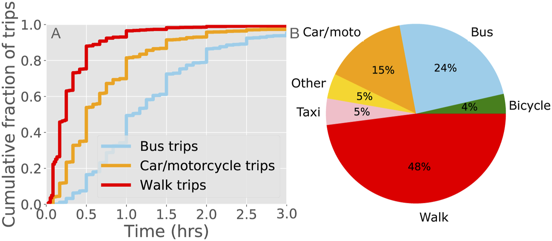

We deploy two related sets of models, one for the probability of mode choice (selection) and the other for trip duration (regression) according to various trip modes. It has been observed that performing selection/regression independently introduces bias in the regression model due to selectivity, and therefore we use Heckman’s correction (Heckman, 1979) in order to fit both models jointly, in similar fashion to Cooke and Ross (1999) and Schwanen et al. (2002). For each trip mode, we model mode selection using a probit model:

\Pr (\mod e_{t} = m) = Φ (α + β \log a c c e s s {(λ)}_{z (t)} + {(s p a t i a l c o n t r o l s)}_{z} + {(t r i p c o n t r o l s)}_{t})

(3)

where t corresponds to a trip, z(t) refers to the zone in which the trip takes place and Φ represents the standard normal distribution function.

For the trip-level controls, we include controls for individual characteristics (age/gender), whether the household has a motorized vehicle, as well as controls for the purpose of the trip (see Data section). Importantly, Heckman’s correction requires that the independent variables in the two equations must not be the exact same. Hence, we drop age, gender and motorized vehicle ownership in the regression equation (4).

For the spatial controls, we include variables corresponding to urban form (i.e. the D’s of the built environment) and SES. For the D’s, we include the following terms – noting that home/jobs are only reported at the more aggregate cell level (see Supplementary SI Sec. 9):

• density_c – the cell-level density of residents’ home locations.

• diversity_c –– the cell-level ratio of home density to job density.

• log dist transit_z – the logarithm of zone-level distance to bus stops/stations.

• design_z – the zone-level density of intersections.

These estimates in equation (3) for the probability of choosing mode m are then transformed via the inverse mills ratio into a variable Λ_t, which is implicitly a function of the independent variables in equation (4). By simultaneously fitting equation (4), we model trip duration for trips of mode m (‘uncensored’ trips) according to the following equation:

\log d u r a t i o n_{t} = α + β \log a c c e s s {(λ)}_{z (t)} + {(s p a t i a l c o n t r o l s)}_{z} + {(t r i p c o n t r o l s)}_{t} + β_{Λ} Λ_{t}

(4)

The coefficient on the inverse mills ratio necessarily depends on the correlation between the residuals of the two equations (Heckman, 1979). We have taken the logarithm of dependent/independent variables of interest in order to compute elasticity as in Ewing and Cervero (2017). For each type of trip modality, we use a maximum likelihood estimation (MLE) framework to fit equations (3)–(4) simultaneously.

We do not include an additional variable for destination accessibility, as we include access(λ) to amenities as our variable of key interest – and further incorporating additional variables results in increased multicollinearity (see SI for a detailed analysis of multicollinearity). In practice, we find considerable multicollinearity between access(λ) and control variables, especially for increasing λ – and hence we limit our analysis to λ ≤ 3. Additionally, we also report regression results when these spatial controls are excluded, calling this model I/II and the full model IA/IIA.

Finally, finding that SES is a modifier for the effect of amenity accessibility on trip behaviour (see SI), we use an effect modification setup for recovering effects of amenities within specific SES groups. That is, we modify equations (3) and (4) to include interaction terms to separate effects of access(λ)_z(t) for different levels of stratum (low: 1–2, medium 3–4 and high 5–6). In this equation, we also include fixed effects for the medium- and high-stratum groups. The normal intercept is kept as a term for the low-stratum group only. We henceforth denote the original model (Equations (3) and (4)) Model I and the model with effect modifier interaction terms Model II.

Results

How are amenities distributed?

Before examining the effect of amenities on urban mobility, we first note that individual amenity classes have differing spatial distributions throughout the city. Even though all classes broadly depend on the distribution of potential customers throughout the city, we would expect, for example, significant differences between the distribution of convenience stores and physiotherapists. And, as observed in Chong et al. (2020), wealthier areas have more diverse amenities (see, for instance, Fig. 2D-E). We investigate these differences in the SI.

While we observe differences in how the various amenity classes are distributed across the city, our metric access(λ) is intended to quantify the composite spatial accessibility to a broad range of amenity classes. However, does the heterogeneity among the amenity distributions render this goal inappropriate? We show in the SI that the first principal component (PC) of the matrix of amenity counts by class and zone explains 75% of the variance. Hence, since the variation in amenity distribution across zones is reasonably well-aligned, we deduce that we can aggregate amenity classes across zones in our accessibility metric.

We display the spatial distribution of accessibility for varying λ in Figure 2(e)–(g). For low λ, we observe a very peaky distribution, with very high density all around the city centre and also many local maxima scattered throughout the study area. As we increase λ, we observe increasing smoothness in the accessibility distribution. Whereas at λ = 0.5 km, we see that amenity hotspots are frequently surrounded by low accessibility zones (e.g. yellow zones surrounded by blue), increasing λ to 1.5 km has the effect of spreading out these hotspots into nearby zones.

Figure 2.

Distribution of amenities in Bogotá. Subfigure (a) enumerates the county of each amenity class throughout the study region. Subfigure (b) shows the spatially averaged stratum (a proxy for SES) of each zone, in addition to the city’s generally recognized city centre. Subfigures (c–d) contrast the building density and amenity intensity of low- and high-stratum areas using satellite imagery. Lower stratum areas are home to many convenience stores (pink points), but lack the diversity of upper stratum areas. Subfigure (e) displays the raw amenity density throughout the city centre, while (f–g) display the distribution of amenity accessibility at two spatial scales. In F, only nearby amenities contribute substantially to the metric, while more distant contributions give rise to a spatially smoother distribution in G.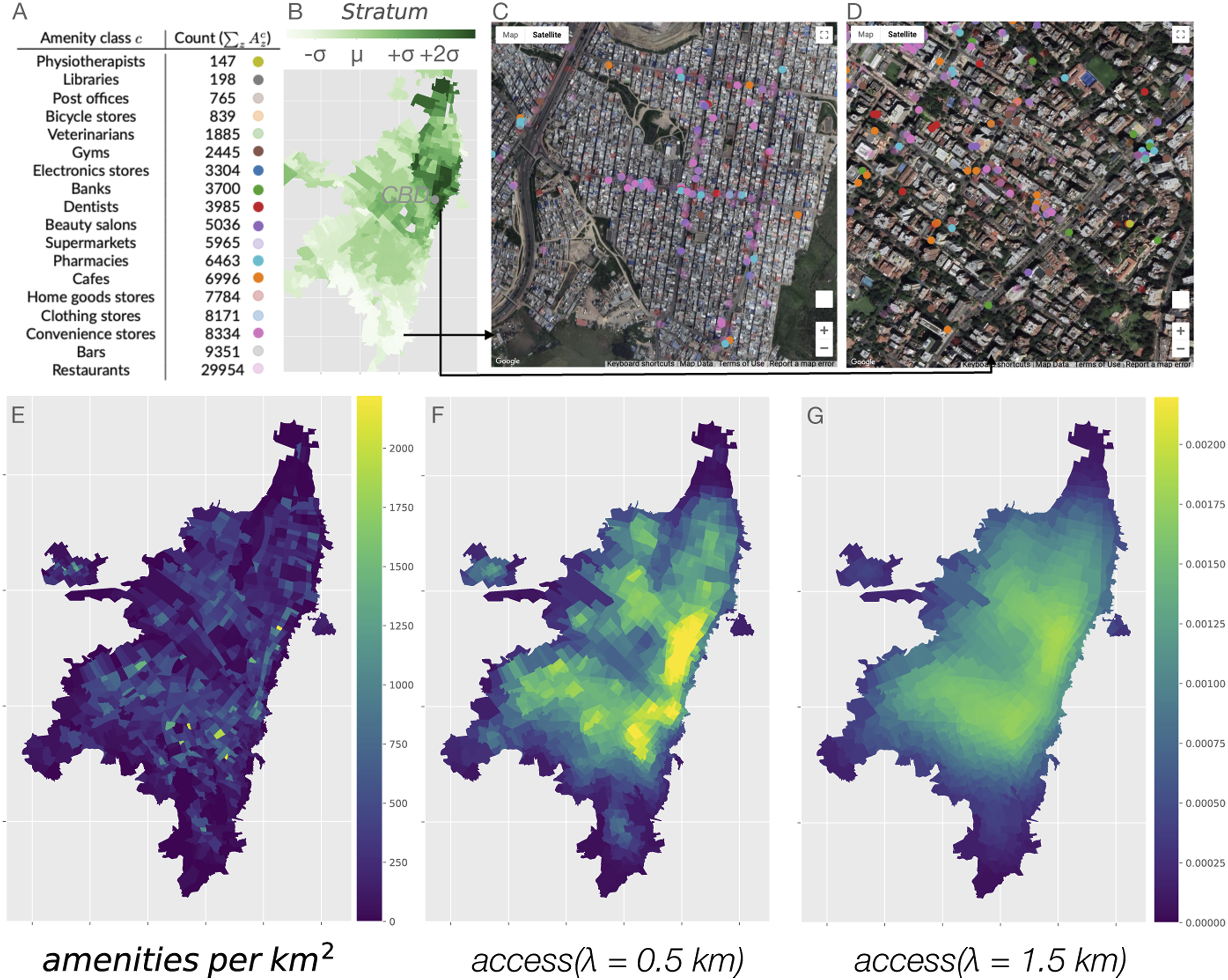

Amenity accessibility impacts mobility behaviour

The primary goal of our work is to further untangle the relationship between accessibility to amenities and urban mobility patterns. For example, does an abundance of local amenities increase our propensity to walk in the local area? Does it reduce the need for long car journeys? We organize our discussion according to trip modes.

Walking

First, we fit equation (3) for the probabilities of walking. Initially, we select a single value of λ, our spatial scale parameter, choosing λ = 0.5 km. We find that higher amenity accessibility is associated with a higher probability of walking for the full sample (first two columns, I-IA, of Table 1), with even stronger results in model IA wherein SES and built environment terms are included as controls. Considering our control variables, we find a negative effect for stratum, indicating that lower SES people are in general more likely to walk (as in Guzman & Bocarejo, 2017)). Unsurprisingly, we find a negative effect for car ownership as those without cars are much likelier to walk (and those with cars less likely to walk). As in Elldér (2020), density and transport proximity coefficients are insignificant when amenities are included, though diversity and street design do significantly increase walking. Women are likelier to walk, perhaps due to childcare and household load (Duchène, 2011).

Table 1.

Effects of access on automotive and car duration.

	Dep. Variable: log duration_t (auto trips)				Dep. Variable: log duration_t (bus trips)
Ind. Variable	(I)	(IA)	(II)	(IIA)	(I)	(IA)	(II)	(IIA)
log access_z(t)(1.5 km)	−0.12***	−0.18***			−0.15***	−0.15***
log access_z(t)(1.5 km)	(0.04)	(0.04)			(0.02)	(0.02)
stratum _z(t)		−0.01				−0.03**
stratum _z(t)		(0.02)				(0.01)
mid stratum _z(t)			−0.37	−0.27			−0.38***	−0.12
mid stratum _z(t)			(0.24	(0.25)			(0.12)	(0.13)
hi stratum _z(t)			−0.58**	−0.53**			0.18	0.40*
hi stratum _z(t)			(0.23)	(0.24)			(0.23)	(0.23)
access × low_z(t)			−0.00	−0.08			−0.11***	−0.15***
access × low_z(t)			(0.07)	(0.08)			(0.02)	(0.03)
access × mid_z(t)			−0.12*	−0.17**			−0.24***	−0.18***
access × mid_z(t)			(0.07)	(0.07)			(0.05)	(0.05)
access × hi_z(t)			−0.19***	−0.27***			0.01	0.03
access × hi_z(t)			(0.06)	(0.07)			(0.09)	(0.09)
density _c(t)		7.5e-6***		6.7e-6**		6.7e-6***		6.9e-6***
density _c(t)		(2.9e-6)		(3.0e-6)		(1.5e-6)		(1.5e-6)
diversity _c(t)		−5.7e-2*		−6.3e-2**		3.7e-2**		4.1e-2**
diversity _c(t)		(3.2e-2)		(3.2e-2)		(1.8e-2)		(1.8e-2)
log dist transit_z(t)		3.5e-2***		3.3e-2***		0.8e-2		0.9e-e−2
log dist transit_z(t)		(1.3e-2)		(1.3e-2)		(1.1e-2)		(1.1e-2)
design _z(t)		−0.9e-4		−0.07e-4-		1.4e-4*		−1.3e-4
design _z(t)		(1.6e-4)		(1.6e-4)		(0.8–4)		(0.8e-4)
Intercept	3.37***	3.09***	3.75***	3.36***	3.90***	3.81***	3.97***	3.75***
Intercept	(0.10)	(0.19)	(0.20)	(0.24)	(0.09)	(0.12)	(0.10)	(0.13)
weekend_t	0.06	0.06	0.06	0.06 0.01	0.02	0.02	0.02
weekend_t	(0.04)	(0.04)	(0.04)	(0.04) (0.02)	(0.02)	(0.02)	(0.02)
dine_t	−0.57***	−0.55***	−0.56***	−0.55***	−0.39***	−0.55***	−0.49***	−0.52***
dine_t	(0.08)	(0.08)	(0.08)	(0.08)	(0.14)	(0.14)	(0.14)	(0.14)
errand_t	−0.24***	−0.24***	−0.25***	−0.24***	−0.13***	−0.16***	−0.15***	−0.15***
errand_t	(0.05)	(0.05)	(0.05)	(0.05)	(0.03)	(0.03)	(0.03)	(0.03)
recreation_t	−0.29***	−0.27***	−0.29***	−0.28***	−0.21***	−0.27***	−0.26***	−0.25***
recreation_t	(0.07)	(0.07)	(0.07)	(0.07)	(0.07)	(0.07)	(0.07)	(0.07)
shopping_t	−0.7***	−0.69***	−0.69***	−0.69***	−0.35***	−0.49***	−0.46***	−0.47***
shopping_t	(0.05)	(0.05)	(0.05)	(0.05)	(0.08)	(0.08)	(0.08)	(0.08)
religious_t	−0.36***	−0.36***	−0.37***	−0.37***	−0.16**	−0.21***	−0.21***	−0.2***
religious_t	(0.11)	(0.11)	(0.11)	(0.11)	(0.08)	(0.08)	(0.08)	(0.08)
physical_t	−0.73***	−0.71***	−0.71***	−0.71***	−0.45***	−0.59***	−0.56***	−0.57***
physical_t	(0.09)	(0.09)	(0.09)	(0.09)	(0.1)	(0.1)	(0.11)	(0.1)
search_t	−0.48***	−0.49***	−0.49***	−0.49***	−0.19***	−0.28***	−0.25***	−0.27***
search_t	(0.08)	(0.08)	(0.08)	(0.08)	(0.07)	(0.07)	(0.07)	(0.07)
Λ	0.13**	0.12**	0.12**	0.12**	0.04	0.19**	0.15*	0.17**
Λ	(0.05)	(0.06)	(0.06)	(0.06)	(0.07)	(0.08)	(0.08)	(0.08)
Obs(total)	15,133	15,133	15,133	15,133	15,133	15,133	15,133	15,133
Obs(censored)	2245	7257	2245	7257	3689	7257	3689	7257
R ²	0.096	0.105	0.102	0.107	0.047	0.060	0.053	0.062

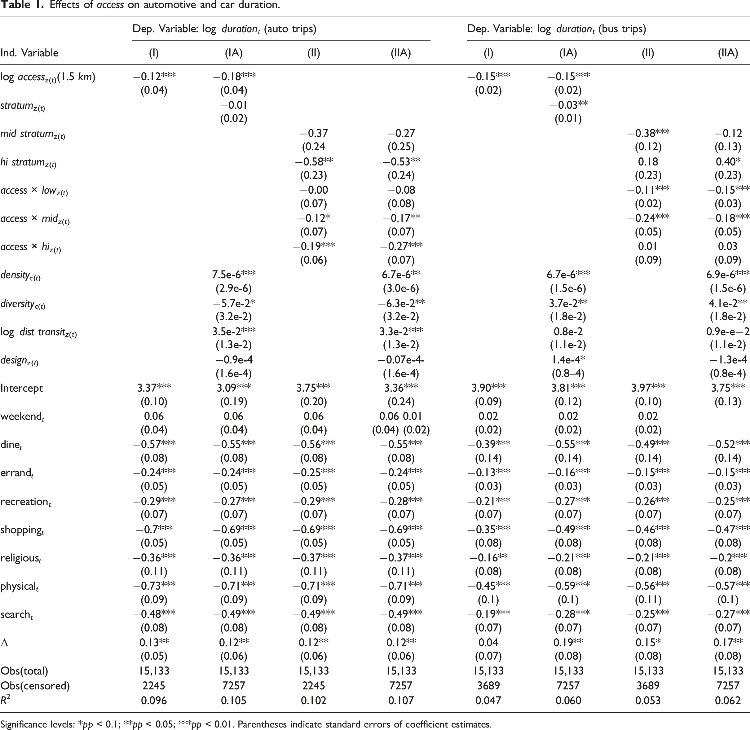
Significance levels: *pp < 0.1; **pp < 0.05; ***pp < 0.01. Parentheses indicate standard errors of coefficient estimates.

Next, we wish to better understand how amenities impact the tendency to make walking trips for specific SES groups. For example, does having amenities nearby have a different influence on trip behaviour for poorer vs richer citizens? That is, we move to our effect modification analysis (Model II), wherein we drop the control for stratum and investigate the interactions between stratum groups and accessibility. We both present the results in the third/fourth columns of Table 1 (Model II/IIA) as well as depict the results visually for model IIA in the upper left panel of Figure 3 (corresponding figures for model II are found in the Supplementary SI Sec. 7).

Figure 3.

Effects of accessibility on tendency to make walking trips (first row) and walking trip duration (bottom). The first column displays the elasticities of log access(λ) at λ = 0.5 km first according to Model IA (no effect modification terms) and then for the various interaction terms in Model IIA. In the second column, we display coefficients/confidence intervals for the full sample as well as SES subgroups (grey corresponding to all respondents, light green corresponding to elasticity within the low-SES subset, etc.). Solid lines indicate significance (p < 0.05), whereas dashed lines indicate insignificance. In the right panel, we plot the probability of walking across increasing deciles of accessibility for each SES group.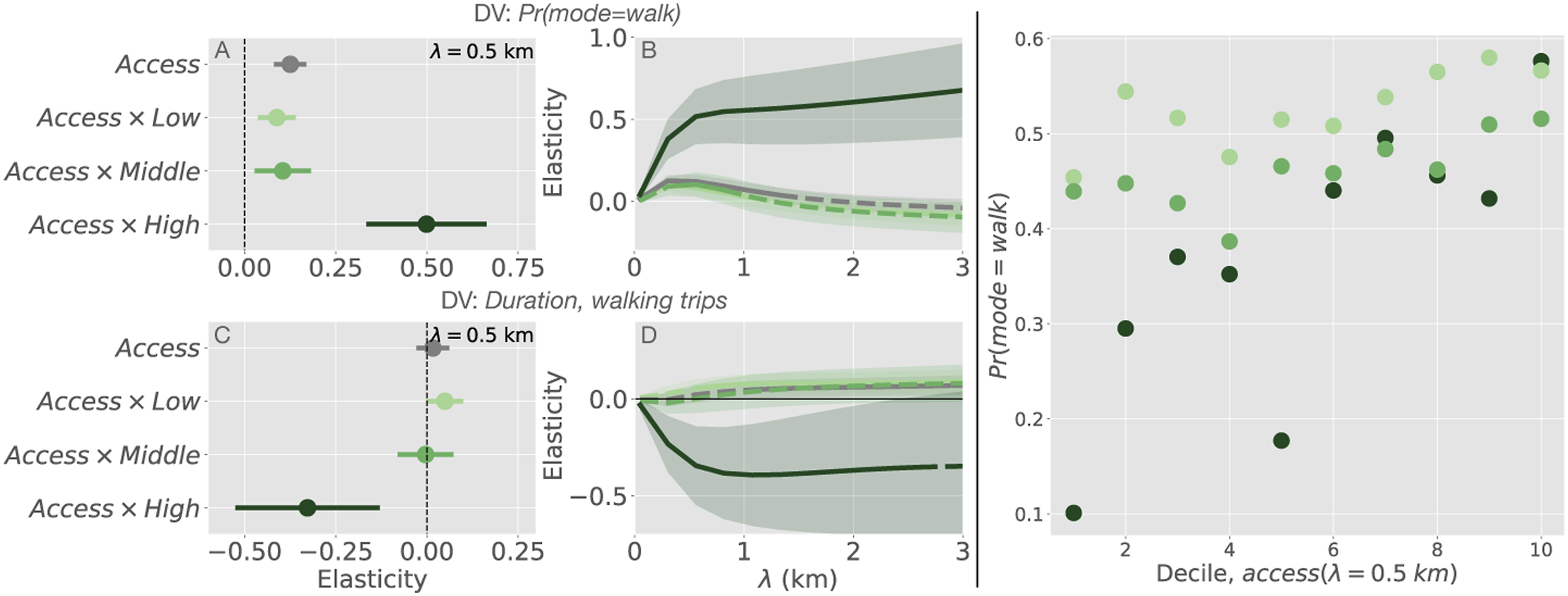

We find that effects of amenities on the likelihood of walking are strongest for the wealthiest group. At λ = 0.5 km (Model IIA), a 1% increase in accessibility results in a 0.50% increase in the likelihood of walking vs about a 0.00−0.10% increase for the lower and middle SES groups (left column of Figure 3).

Our results point toward an important role for amenities in the mobility behaviour of high-SES residents, but less so for low/middle SES residents. In order to illustrate this, we compute Pr(walk) for each decile of accessibility for each SES group in the right panel of Figure 3. For the high-SES group, we find that the probability to walk clearly increases with accessibility. In contrast, we observe at best a weak pattern for the low- and middle-SES groups.

We also consider variation in the spatial scale parameter λ for the effect of amenity accessibility on walking trip propensity. Specifically, we examine the elasticity of amenity accessibility as a function of λ on trip mode propensity (see second column of Figure 3). A peak for smaller values of λ implies that only close-by amenities are associated with trip behaviour, whereas a peak for a larger value means that amenity hotspots within the general area of the city play a role.

The high-SES group exhibits a strong association between amenity accessibility and the probability of walking. The coefficient for this group increases significantly between λ = 0.1 − 0.7 km and then more or less levels off with no further significant increase. This suggests that nearby amenities heavily influence walking for this group, while more distant amenities have little additional influence. The coefficient for the other two groups peak for small λ, and both become insignificant for higher λ. Again, this suggests that only nearby amenities influence the propensity to walk for these groups.

In addition, we investigate effects on walking duration – which we fit according to equation (4) simultaneously with equation (3) via MLE. Again, we first choose λ = 0.5 km and later investigate effects for varying λ, reporting results in the right four columns of Table 1 and depicting them visually in Figure 3. The coefficient of accessibility for the full sample is insignificant for all λ – suggesting that while amenities do influence people to walk, they do not reduce the length of the walking trip in general. This is not so surprising: walkers in amenity-rich areas may not seek to minimize time as they are more likely to be taking recreational trips and visiting multiple amenities (trip chaining). Nor do we find significant effects for stratum or for most built environment controls, with the exception of street design. We do find significant effects for the inverse mills ratio, indicating that modeling walking propensity and walking duration independently (i.e. without our use of Heckman’s correction) would result in selection bias.

We do find some differences in the effects of accessibility on walking duration for the various socioeconomic groups. That is, we find that there is no significant effect for the low/middle SES groups, but find evidence for a reducing effect for the high-SES group. That is, a 1% increase in amenity accessibility for this group is associated with a corresponding 0.33% decrease in walking duration (Model IIA). These findings seem to hold across a broad range of λ. Hence, higher amenity accessibility is significantly associated with shorter walking trips for high-SES residents, but it has no effect on walking duration for the low- and middle-SES groups.

Overall, we find that higher amenity accessibility is associated with a higher probability of walking but has very little effect on walking trip duration. By far, the strongest effects for walking propensity emerge for the wealthiest group. The coefficient for the high-SES group tends to increase until about 0.7 km, at which point it levels off.

Car and motorcycle

How does the presence of amenities influence the probability of taking other modes of transport besides walking? If amenities increase the probability of walking, then they decrease the probability of not walking, for example, travelling by car or bus. In the SI (Supplementary Sec. 6), we show that this is the case: amenity accessibility is (for all spatial scales) associated with lower probability of taking the bus, or – for the wealthy subgroup only – the car. Unexpectedly, more amenities actually mean a higher probability of driving versus taking the bus for the low-SES group.

We focus here on car trip duration, displaying results in the left columns of Table 2 and in the top row of Figure 4. As above, we first select a single value of our spatial scale parameter λ. We choose λ = 1.5 km as we a priori expect a larger spatial scale to be more appropriate for investigating bus trip behaviour. At λ = 1.5 km, we find that in the full sample accessibility to amenities is associated with reduced car trip duration. The elasticity is fairly similar whether or not we control for stratum and built environment factors ( − 0.12/− 0.18 for models I/IA). Higher density and diversity, likely signalling effects of congestion, while being further from a bus stop are associated with increased duration. However, we observe no significant effect of SES. Here, we do observe a significant effect for the inverse mills ratio.

Table 2.

Effects of access on walking behaviour.

	Dep. Variable: Pr(walk)_t				Dep. Variable: log duration_t (walking trips)
Ind. Variable	(I)	(IA)	(II)	(IIA)	(I)	(IA)	(II)	(IIA)
log access_z(t)(0.5 km)	0.07***	0.14***			0.01	0.01
log access_z(t)(0.5 km)	(0.02)	(0.02)			(0.01)	(0.02)
stratum _z(t)		−0.12***				0.01
stratum _z(t)		(0.01)				(0.01)
mid stratum _z(t)			−0.26**	−0.15*			−0.19**	−0.13
mid stratum _z(t)			(0.10)	(0.11)			(0.09)	(0.10)
hi stratum _z(t)			0.53***	0.64***			−0.86***	−0.79***
hi stratum _z(t)			(0.20)	(0.20)			(0.20)	(0.21)
access × low_z(t)			0.12***	0.10***			0.04**	0.05**
access × low_z(t)			(0.02)	(0.03)			(0.02)	(0.02)
access × mid_z(t)			0.11***	0.11***			−0.04	−0.00
access × mid_z(t)			(0.04)	(0.04)			(0.03)	(0.04)
access × hi_z(t)			0.56***	0.55***			−0.35***	−0.33***
access × hi_z(t)			(0.09)	(0.09)			(0.09)	(0.10)
density _c(t)		2.4e-6		2.6e-6		2.1e-6		1.8e-6
density _c(t)		(1.6e-6)		(1.7e-6)		(1.4e-6)		(1.4e-6)
diversity _c(t)		2.2e-2**		1.2e-2		−0.7e-2		−0.1e-2
diversity _c(t)		(1.0e-2)		(1.1e-2)		(1.0e-2)		(1.0e-2)
log dist transit_z(t)		1.7e-2		3.2-2		2.6e-2		2.2-e2
log dist transit_z(t)		(1.9e-2)		(1.9e-2)		(1.7e-2)		(1.7e-2)
design _z(t)		2.1-4**		2.3e-4**		−1.5e-4*		−1.5e-4*
design _z(t)		(0.9e-4)		(0.8e-4)		(0.8e-4)		(0.8e-4)
has car_t	−0.45***	−0.36***	−0.38***	−0.38***
has car_t	(0.02)	(0.02)	(0.02)	(0.02)
female_t	0.24***	0.24***	0.24***	0.24***
female_t	(0.02)	(0.02)	(0.02)	(0.02)
age_t	3.8e-3***	4.9e-3***	4.7e-3***	4.7e-3***
age_t	(0.6e-3)	(0.6e-3)	(0.6e-3)	(0.6e-3)
Intercept	−1.15***	−0.89***	−0.95***	−1.17***	3.72***	3.90***	3.93***	3.99***
Intercept	(0.06)	(0.11)	(0.08)	(0.12)	(0.09)	(0.12)	(0.09)	(0.12)
weekend_t	−0.06***	−0.05**	−0.05**	−0.05**	−0.02	−0.02	−0.02	−0.02
	(0.02)	(0.02)	(0.02)	(0.02)	(0.02)	(0.02)	(0.02)	(0.02)
dine_t	1.53***	1.59***	1.57***	1.58***	−1.02***	−1.12***	−1.08***	−1.08***
dine_t	(0.06)	(0.06)	(0.06)	(0.06)	(0.08)	(0.08)	(0.08)	(0.08)
errand_t	0.78***	0.79***	0.79***	0.79***	−0.45***	−0.5***	−0.48***	−0.48***
errand_t	(0.04)	(0.04)	(0.04)	(0.04)	(0.06)	(0.06)	(0.06)	(0.06)
recreation_t	1.2***	1.25***	1.25***	1.26***	−0.74***	−0.82***	−0.79***	−0.79***
recreation_t	(0.05)	(0.05)	(0.05)	(0.05)	(0.07)	(0.07)	(0.07)	(0.07)
shopping_t	1.89***	1.89***	1.89***	1.89***	−1.13***	−1.25***	−1.21***	−1.22***
shopping_t	(0.04)	(0.04)	(0.04)	(0.04)	(0.07)	(0.07)	(0.07)	(0.07)
religious_t	1.29***	1.3***	1.3***	1.3***	−0.78***	−0.87***	−0.84***	−0.84***
religious_t	(0.06)	(0.06)	(0.06)	(0.06)	(0.08)	(0.08)	(0.08)	(0.08)
physical_t	1.9***	1.95***	1.94***	1.95***	−0.91***	−1.02***	−0.99***	−0.99***
physical_t	(0.05)	(0.05)	(0.05)	(0.05)	(0.07)	(0.07)	(0.07)	(0.07)
search_t	1.21***	1.19***	1.19***	1.19***	−0.85***	−0.93***	−0.90***	−0.90***
search_t	(0.06)	(0.06)	(0.06)	(0.06)	(0.08)	(0.07)	(0.07)	(0.07)
Λ					−0.29***	−0.38***	−0.35***	−0.36***
Λ					(0.05)	(0.05)	(0.05)	(0.05)
Obs(total)	15,133	15,133	15,133	15,133	15,133	15,133	15,133.0	15,133
Obs(censored)					7257	7257	7257	7257
Pseudo − R²	0.205	0.213	0.212	0.213
R ²					0.068	0.072	0.072	0.073

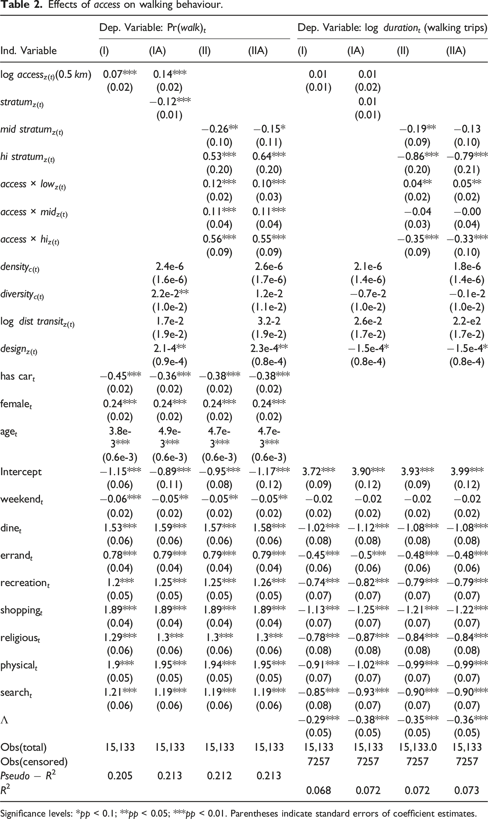
Significance levels: *pp < 0.1; **pp < 0.05; ***pp < 0.01. Parentheses indicate standard errors of coefficient estimates.

Figure 4.

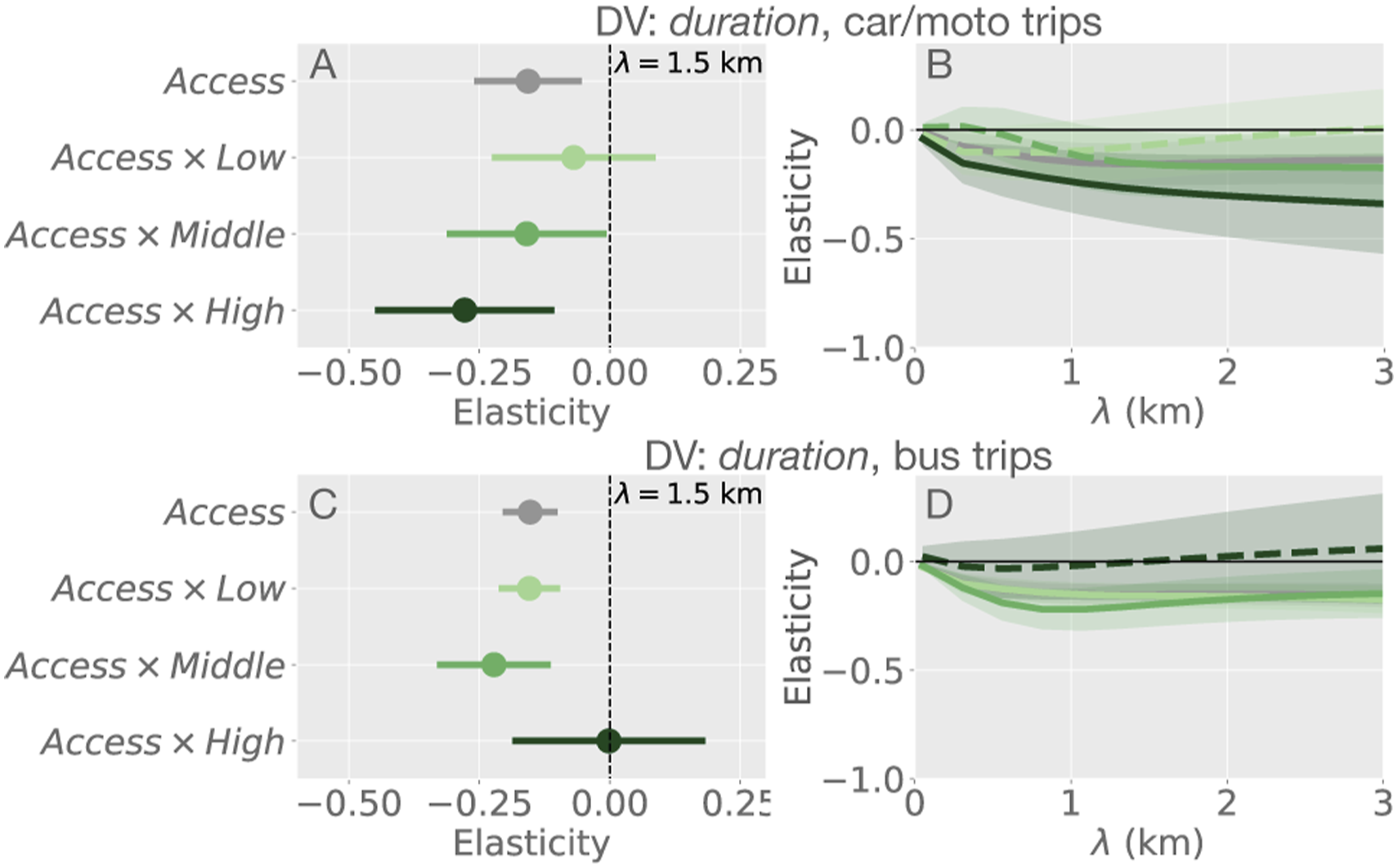
Effects of amenity accessibility on bus and auto trip duration. Rows correspond to effects on the various dependent variables. For each row, the left column displays the elasticity/confidence intervals for log access effects at fixed λ both for all respondents and then for low/middle/high SES groups. The right column displays the elasticity when we let λ vary across a range of spatial scales.

By disaggregating effects by SES group, we find that at λ = 1.5 km, amenity accessibility is only associated at the p < 0.05 level with reduced car trips for the upper- and middle-SES groups. The effect is substantially stronger for the high-SES group. When we vary λ, we see a robust effect for the high-SES group, but the middle-SES group coefficient is only significant for λ > 1.2. As above, both of these coefficients initially increase in magnitude for increasing λ, but gradually level off. The low-SES group coefficient is not significant for any λ.

Hence, it seems that the association of amenity accessibility and car trip duration is modified by SES. That is, for high- and perhaps middle-SES residents, having more amenities nearby is associated with reduced car trip duration. However, there is no significant association between amenities and car trip duration for the low-SES group.

Bus

Regarding bus trips, we find that higher amenity accessibility is associated with shorter bus trips, with or without built environment controls (see right four columns of Table 2 and the second row of Figure 4). In fact, our results are strikingly similar between models I and II here, with the elasticity of amenity accessibility being − 0.15 in both cases. Hence, bus trips beginning in areas of the city with higher amenity accessibility tend to be shorter. SES has a robust negative effect on bus trip duration, meaning that higher stratum residents take shorter bus trips. On the other hand, density and diversity are again associated with longer trips, perhaps signalling congestion. Distance to transit doesn’t seem to greatly affect bus trip duration – as we show in the SI (Supplementary Sec. 9), this distance does not vary greatly across most of the study area and hence may be less informative. Effects for trip purpose are generally significant, and the significance of the inverse mills ratio (Λ) varies by model.

When we examine specific SES groups, we see that this negative effect on bus trip duration holds for the low- and middle-SES groups, but does not extend to the high-SES group. Next, we vary the spatial scale parameter λ. Focusing first on the full sample (grey), the coefficient decreases steadily with increasing λ until about 0.7 km, at which point the coefficient seems to level off. This suggests that amenities within about 0.7 km are most associated with lower bus trip duration. Looking at the individual SES groups, we see that for low/middle SES groups, the coefficient tends to exhibit similar behaviour as in the model without effect modification, while the upper SES coefficient is insignificant for all λ. The middle-SES group coefficient tends overall to be slightly stronger than the lower-SES group coefficient.

Here, we find that amenities are associated with reduced bus trip duration for the low- and middle-SES groups, but not for the high-SES group. As is the case with car trip duration, effects on bus trip duration tend to increase in magnitude with the spatial scale λ until around 0.7 km before leveling off.

Discussion

In this paper, we investigate the role of socioeconomic status in the relationship between local amenities and mobility patterns. In particular, we leverage data from a large internet repository of location data on amenities and use this to construct an amenity accessibility measure. Our results show that on the whole, having more amenities nearby leads to a modest reduction in car and bus travel distance and increases residents’ tendency to walk, in line with other recent work on amenities in Sweden (Elldér, 2020; Elldér et al., 2020; Haugen & Vilhelmson, 2013). However, SES seems to modulate this relationship in an important and hitherto unrecognized manner. Specifically, we find that the presence of amenities increases walking trip propensity and decreases car travel duration for the wealthiest group only. Effects are either insignificant or very small in magnitude for the lower- and middle-SES groups. On the other hand, amenities tend to reduce bus trip duration (which has been studied less in this literature) for just the low- and middle-income SES groups.

We suspect that different socioeconomic groups make travel mode decisions based on different factors, particularly in the case of walking. In addition to being much more likely to walk overall, low-income people are thought to choose walking for different reasons than wealthy people (Boarnet and Crane, 2001; Mondschein, 2018). For example, lower income people may see the cost of driving or taking a bus as a more costly alternative and factor this cost more heavily into their decision to walk. A longer walking trip may be more preferable than paying a bus fare or paying for gas – lowering sensitivity to the immediate amenity supply. By contrast, this cost weighs less heavily on the wealthy, and their decision to walk may depend less on cost and more on the proximity to amenities. Wealthier suburban residents with relatively few amenities nearby can much more efficiently get what they need by driving than by walking. By contrast, inner-city high-SES residents live in amenity-rich ‘walkable’ neighbourhoods and are hence much likelier to walk. This narrative is consistent with our results which highlight the much stronger effect of amenities on the tendency of the wealthy to walk relative to the low- and middle-SES groups.

Our measure captures average accessibility across all amenity types, but one possible confounding factor is that people residing in lower SES areas may be more separated from the specific amenities that they need or wish to access. Indeed, more specialized amenities tend to be rarer in low-SES areas, as we confirm and elucidate in Supplementary SI Sec. 10. Previous research has shown that poorer neighbourhoods have lower accessibility to banking and more access to alternative financial institutions (e.g. payday lenders) in the US (Small et al., 2021), so residents needing, for example, mortgage advice would need to travel further even when the composite local amenity supply is higher. Additionally, it is well known that poorer areas are often associated with more fast food and fewer supermarkets (Sharkey et al., 2009), and so local residents may be travelling further for their own needs which are not met by the local amenity supply. This topic merits further attention – for instance, our work could be adapted to further examine effects of specific amenity classes on trip behaviour (similar to Elldér et al., 2020). Additionally, specific amenity accessibilities could be matched to particular trip types (e.g. shopping trips to specific retail amenity classes).

Our accessibility measure was constructed specifically to measure proximity to amenities at various spatial scales. A priori we might expect that close-by amenities would influence the propensity to walk, whereas further away amenities might impact car trip duration. However, in our analysis, we find similar behaviour with regards to spatial scale for all three modes studied. Specifically, the coefficients peak in a short range of 0.5–1 km and then typically level off. We could interpret this as suggesting, for example, in the case of car trip duration, is that what matters is not so much the presence of further away amenities, but the absence of nearby amenities. This topic merits further study and perhaps a more sophisticated framework for amenity accessibility that takes into account local versus regional amenities as well (similar to Haugen and Vilhelmson, 2013).

Finally, we point to some limitations of this work, primarily related to data availability. First, we note issues of spatial aggregation. While the zone sizes we use are relatively small relative to the city (median area 0.38 km²) and relative to units used in peer studies in Sweden⁴ (Amcoff, 2012; Elldér, 2020; Elldér et al., 2020), walking behaviour in particular may depend on a very granular spatial scale (Handy et al., 2002). For instance, supposing the median cell is a circle with all amenities in its centre, two respondents in the same median-size zone have the same amenity accessibility value when in reality one respondent residing in the centre would be $\sqrt{. 38 / π} \sim . 35$ km closer to amenities than a respondent residing on the edge. This difference hardly seems significant for explaining driving duration, but it may be more important for modal choice and walking duration. While the spatially continuous nature of our amenity accessibility metric makes it much less sensitive to MUAP issues than measures that only consider interior amenities (see Figure 2(e)-(g)), the resolution of our accessibility metric is dependent on having small zones. Also, with sufficient data, our accessibility metric could perhaps be improved by replacing distance to amenities with travel duration in equation (1). Additionally, a lack of spatial resolution in measurement of homes/jobs, which are measured at the cell level, limits our ability to control for density and diversity. In order to confirm our findings and to better understand drivers of urban travel behaviour, we point to a need to replicate our findings in other cities or – even better – to use a temporal rather than a cross-sectional experimental setup as in Naess (2014).

Moreover, while the five D’s of the built environment are the most studied influences on transport behaviour especially in Global North cities, perception of traffic safety and security are both undoubtedly very important for transport decisions, particularly in Latin America (Arellana et al., 2020). Future work might look to examine how different SES groups take safety and security into account in their transport behaviour, perhaps using a similar modelling framework to our own.

Conclusions and policy implications

Overall, our results suggest that low-income groups’ walking and driving behaviour depend less on the availability of neighbourhood amenities within their local environment relative to wealthy residents. This result somewhat contrasts previous characterizations of the poor as being more connected to their local environment when it comes to transport behaviour (Marquet et al., 2017), although we note that commercial development is only one dimension of the local environment. For instance, in the context of urban health, many studies show that the relationship between the local environment and health is stronger for low-income people (Vallée et al., 2021).

These findings generate important nuance in the debate on the development of more walkable neighbourhoods via bringing residents closer to amenities (‘15 minute cities’ or ‘walkable mixed use communities’). While our study is cross-sectional, our results suggest that adding amenities to a low-income or a wealthy neighbourhood may have different effects on residents’ transport behaviour. In a wealthy area, amenities alone may drive residents to walk much more. However, while amenities provide many types of neighbourhood benefits beyond the scope of this study, other neighbourhood improvements may be more impactful when it comes to changing travel behaviour for low- and middle-income communities.

Supplemental Material

Supplemental Material – Are neighbourhood amenities associated with more walking and less driving? Yes, but predominantly for the wealthy

Supplemental Material for Are neighbourhood amenities associated with more walking and less driving? Yes, but predominantly for the wealthy by Samuel Heroy, Isabella Loaiza, Alex Pentland and Neave O’Clery in Environment and Planning B: Urban Analytics and City Science.

Footnotes

Acknowledgements

The authors would like to thank Tim Schwanen (Professor of Transport Studies, University of Oxford) for helpful comments and especially analytical suggestions, as well as the editor Seraphim Alvanides (Associate Professor of Architecture and the Built Environment, Northumbria University) and three anonymous referees. All errors are those of the authors alone. The views expressed in this paper do not necessarily reflect the position of the Federal Reserve Bank of Richmond or the Federal Reserve System.

Declaration of conflicting interests

The author(s) declared no potential conflicts of interest with respect to the research, authorship and/or publication of this article.

Funding

The author(s) disclosed receipt of the following financial support for the research, authorship and/or publication of this article. SH and NO acknowledge support from the PEAK Urban programme, funded by UKRI’s Global Challenge Research Fund, Grant Ref: ES/P011055/1.

ORCID iD

Samuel Heroy

Supplemental Material

Supplemental material for this article is available online.

Notes

Samuel Heroy is a quantitative fellow in the Quantitative Supervision and Research group of the Federal Reserve Bank of Richmond. His primary research interest outside bank supervision involves using mobile phone data to understand city structure, resilience, and disaster scenarios. Previously, he worked as a postdoctoral researcher at the University of Oxford and University College London, and as a data science consultant for the World Bank. He holds a PhD in applied mathematics from the University of North Carolina at Chapel Hill.

Isabella Loaiza is a Research Assistant at the MIT Media Lab. Her work focuses on using data to understand how individuals and groups make impactful decisions related to careers, relocation and economic trade, and building human-centered tools that support these decisions.

Professor Alex ‘Sandy’ Pentland directs MIT Connection Science, an MIT-wide initiative, and previously helped create and direct the MIT Media Lab and the Media Lab Asia in India. He is one of the most-cited computational scientists in the world, and Forbes declared him one of the “7 most powerful data scientists in the world” along with Google founders and the Chief Technical Officer of the United States. He is on the Board of the UN Foundations' Global Partnership for Sustainable Development Data, co-led the World Economic Forum discussion in Davos that led to the EU privacy regulation GDPR, and was one of the UN Secretary General's “Data Revolutionaries” helping to forge the transparency and accountability mechanisms in the UN's Sustainable Development Goals.

Neave O’Clery is Associate Professor and Director of Research at the Centre for Advanced Spatial Analysis (CASA) at University College London where she leads a research group focused on data-driven models for economic development, complex systems and cities. She also works alongside a wide variety of policy-makers ranging from local government to global multilaterals such as the World Bank. In 2022, she won the annual Complex Systems Society Junior Award. She was previously a Senior Research Fellow at the Mathematical Institute at the University of Oxford, and before this a Fulbright Scholar at the Center for International Development at the Harvard Kennedy School following her PhD (mathematics) at Imperial College.

References

Adler

Vera

Wainer

, et al. (2018) Housing What’s Next?: From Thinking the Unit to Building the City. Washington, DC: Inter-American Development Bank.

Advisors

(2021) Montgomery County Mixed-Use Development Study. Wheaton, MD: Montgomery County Planning Department. https://montgomeryplanning.org/wp-content/uploads/2021/07/Montgomery-County-Mixed-Use-Study-7-12-21_FINAL.pdf

Agrawal

Schimek

(2007) Extent and correlates of walking in the usa. Transportation Research Part D: Transport and Environment 12(8): 548–563.

Amcoff

(2012) Hur bra fungerar samsområdena i studier av grannskapseffekter? en studie av samsområdenas homogenitet. Socialvetenskaplig Tidskrift 19(2): 2450.

Anguelovski

Irazábal-Zurita

Connolly

(2019) Grabbed urban landscapes: Socio-spatial tensions in green infrastructure planning in medellín. International Journal of Urban and Regional Research 43(1): 133–156.

Arellana

Saltarín

Larrañaga

, et al. (2020) Urban walkability considering pedestrians’ perceptions of the built environment: a 10-year review and a case study in a medium-sized city in latin america. Transport Reviews 40(2): 183–203.

Ashik

Mim

Neema

(2020) Towards vertical spatial equity of urban facilities: An integration of spatial and aspatial accessibility. Journal of Urban Management 9(1): 77–92.

Bank

(2015) Master Planning. Washington, DC: World Bank. https://urban-regeneration.worldbank.org/node/51

Barbosa

Hazarie

Dickinson

, et al. (2021) Uncovering the socioeconomic facets of human mobility. Scientific Reports 11(1): 1–13.

10.

Boarnet

Crane

(2001) Travel by Design: The Influence of Urban Form on Travel. Oxford, England: Oxford University Press on Demand.

11.

Bocarejo

Escobar

Hernandez

, et al. (2016) Accessibility analysis of the integrated transit system of bogotá. International Journal of Sustainable Transportation 10(4): 308–320.

12.

Bogotá y municipios vecino (2019) Resultados de la encuesta de movilidad de bogotá y municipios vecinos. Bogotá: Bogotá y municipios vecino.

13.

Bogotá y municipios vecino (2020) Traffic Index 2020. Bogotá: Bogotá y municipios vecino. https://www.tomtom.com/en_gb/traffic-index/ranking/

14.

Cantillo-García

Guzman

Arellana

(2019) Socioeconomic strata as proxy variable for household income in transportation research. evaluation for bogotá, medellín, cali and barranquilla. Dyna 86(211): 258–267.

15.

Carlino

Saiz

(2019) Beautiful city: Leisure amenities and urban growth. Journal of Regional Science 59(3): 369–408.

16.

Cherednichenko

(2021) Best Map Api for Location-Based Services: Mapbox vs Google Maps vs Openstreetmap. Ukraine: Relevant Software LLC. https://medium.com/mobindustry/best-map-api-for-location-based-services-mapbox-vs-google-maps-vs-openstreetmap-4199fbd6d5d3

17.

Chong

Bahrami

Chen

, et al. (2020) Economic outcomes predicted by diversity in cities. EPJ Data Science 9(1): 17.

18.

Cooke

Ross

(1999) Sample selection bias in models of commuting time. Urban Studies 36(9): 1597–1611.

19.

Departamento Administrativo Nacional de Estadística (DANE) (2020) Censo nacional de población y vivienda.Colombia: National Administrative Department of Statistics. https://www.dane.gov.co/index.php/en/estadisticas-por-tema/demografia-y-poblacion/censo-nacional-de-poblacion-y-vivenda-2018

20.

Department for Levelling Up HC (2021) Build Back Better High Streets. London: Department for Levelling Up, Housing and Communities. UK Government Policy Paper https://www.gov.uk/government/publications/build-back-better-high-streets/build-back-better-high-streets

21.

Duchène

(2011) Gender and Transport. Paris, France: OECD.

22.

Duranton

(2016) Agglomeration effects in colombia. Journal of Regional Science 56(2): 210–238.

23.

Elldér

Haugen

Vilhelmson

(2020) When Local Access Matters: A Detailed Analysis of Place, Neighbourhood Amenities and Travel Choice. Urban Studies 59: 120–139.

24.

Elldér

(2020) What kind of compact development makes people drive less? the “ds of the built environment” versus neighborhood amenities. Journal of Planning Education and Research 40(4): 432–446.

25.

Ewing

Cervero

(2001) Travel and the built environment: a synthesis. Transportation Research Record 1780(1): 87–114.

26.

Ewing

Cervero

(2017) does compact development make people drive less?” the answer is yes. Journal of the American Planning Association 83(1): 19–25.

27.

Ewing

Tian

Goates

, et al. (2015) Varying influences of the built environment on household travel in 15 diverse regions of the united states. Urban Studies 52(13): 2330–2348.

28.

Ewing

Tian

Lyons

(2018) Does compact development increase or reduce traffic congestion? Cities 72: 94–101.

29.

Ewing

(1997) Is los angeles-style sprawl desirable? Journal of the American Planning Association 63(1): 107–126.

30.

Freemark

(2018) Challenges in the creation of mixed-use affordable housing: Measuring and explaining its limited prevalence. Housing Policy Debate 28(6): 1004–1021.

31.

Glaeser

Kolko

Saiz

(2001) Consumer city. Journal of Economic Geography 1(1): 27–50.

32.

Grant

(2002) Mixed use in theory and practice: Canadian experience with implementing a planning principle. Journal of the American Planning Association 68(1): 71–84.

33.

Guzman

Bocarejo

(2017) Urban form and spatial urban equity in bogota, colombia. Transportation Research Procedia 25: 4491–4506.

34.

Guzman

Oviedo

Rivera

(2017) Assessing equity in transport accessibility to work and study: The bogotá region. Journal of Transport Geography 58: 236–246.

35.

Guzman

Oviedo

Bocarejo

(2017) City profile: The bogotá metropolitan area that never was. Cities 60: 202–215.

36.

Guzman

Oviedo

Cardona

(2018) Accessibility changes: Analysis of the integrated public transport system of bogotá. Sustainability 10(11): 3958.

37.

Guzman

Arellana

Oviedo

, et al. (2021) Covid-19, activity and mobility patterns in bogotá. are we ready for a ‘15-minute city. Travel Behaviour and Society 24: 245–256.

38.

Handy

Boarnet

Ewing

, et al. (2002) How the built environment affects physical activity: views from urban planning. American Journal of Preventive Medicine 23(2): 64–73.

39.

Handy

Cao

Mokhtarian

(2005) Correlation or causality between the built environment and travel behavior? evidence from northern california. Transportation Research Part D: Transport and Environment 10(6): 427–444.

40.

Handy

(1993) Regional versus Local Accessibility: Implications for Nonwork Travel. Transportation Research Record. Washington, DC: Transportation Research Board. pp. 58–66.

41.

Handy

(2017) Thoughts on the meaning of mark stevens’s meta-analysis. Journal of the American Planning Association 83(1): 26–28.

42.

Handy

(2018) Enough with the “Ds” Already — Let’s Get Back to “A”. Transport Reviews.

43.

Haugen

Vilhelmson

(2013) The divergent role of spatial access: The changing supply and location of service amenities and service travel distance in sweden. Transportation Research Part A: Policy and Practice 49: 10–20.

44.

Heckman

(1979) Sample selection bias as a specification error. Econometrica: Journal of the Econometric Society: 153–161.

45.

Hidalgo

Pereira

Estupiñán

, et al. (2013) Transmilenio brt system in bogota, high performance and positive impact–main results of an ex-post evaluation. Research in Transportation Economics 39(1): 133–138.

46.

Hidalgo

Castañer

Sevtsuk

(2020) The amenity mix of urban neighborhoods. Habitat International 106: 102205.

47.

Hunter

Garcia

de Sa

, et al. (2021) Effect of covid-19 response policies on walking behavior in us cities. Nature Communications 12(1): 1–9.

48.

Koschinsky

Talen

Alfonzo

, et al. (2017) How walkable is walker’s paradise? Environment and Planning B: Urban Analytics and City Science 44(2): 343–363.

49.

Kramer

(2013) Our Built and Natural Environments: A Technical Review of the Interactions Among Land Use, Transportation, and Environmental Quality. Washington, DC: US Environmental Protection Agency.

50.

Lin

Geertman

, et al. (2021) Accessibility-based equity of public facilities: A case study in xiamen, china. Applied Spatial Analysis and Policy 14(4): 947–968.

51.

Marquet

Bedoya

Miralles-Guasch

(2017) Local accessibility inequalities and willingness to walk in latin-american cities: Findings from medellín, colombia. International Journal of Sustainable Transportation 11(3): 186–196.

52.

Molina

(2014) Expansión urbana y cambio climático. Ciencia-Academia Mexicana de Ciencias 65(4): 10–13.

53.

Moloney

(2015) Mcolombia’s Medellin Pushes Slum Renewal in Shadow of Gangs. Reuters. https://www.reuters.com/article/us-development-goals-colombia-cities-idUSKCN0RA01B20150910

54.

Mondschein

(2018) Persistent differences in walking across the socioeconomic spectrum: Variations by trip purpose. Journal of Planning Education and Research 41: 445–460.

55.

Morales

Medina

Nuñez

(2008) Quality of Life in Urban Neighborhoods in colombia: The Cases of Bogotá and Medellín. Borradores de Economía, p. 536. Banco de la Republica de Colombia.

56.

Moreno

Allam

Chabaud

, et al. (2021) Introducing the “15-minute city”: Sustainability, resilience and place identity in future post-pandemic cities. Smart Cities 4(1): 93–111.

57.

Moss

(2015) Medellín’s parques del rio project seeks to transform urban civic life – 1st phase on track for january completion. Colombia: Finance Colombia https://www.financecolombia.com/medellins-parque-del-rio-project-seeks-to-transform-urban-civic-life-1st-phase-on-track-for-january-completion/

58.

Næss

Røe

Larsen

(1995) Travelling distances, modal split and transportation energy in thirty residential areas in oslo. Journal of Environmental Planning and Management 38(3): 349–370.

59.

Næss

(2006) Accessibility, activity participation and location of activities: Exploring the links between residential location and travel behaviour. Urban Studies 43(3): 627–652.

60.

Naess

(2014) Tempest in a teapot: The exaggerated problem of transport-related residential self-selection as a source of error in empirical studies. Journal of Transport and Land Use 7(3): 57–79.

61.

Nyerges

Couclelis

McMaster

(2011) The SAGE Handbook of GIS and Society. Thousand Oaks, CA: Sage Publications.

62.

Öner

(2017) Retail city: the relationship between place attractiveness and accessibility to shops. Spatial Economic Analysis 12(1): 72–91.

63.

Ortego

(2015) ‘chaos? This Is Open-Heart Surgery’: Medellín Risks a Massively Expensive Plan to Bury its Highway. The Guardian. https://www.theguardian.com/cities/2015/may/01/medellin-bury-highway-urban-intervention

64.

Paul

Carlson

Carroll

, et al. (2015) Walking for transportation and leisure among us adults—national health interview survey 2010. Journal of Physical Activity and Health 12(s1): S62–S69.

65.

Quastel

Moos

Lynch

(2012) Sustainability-as-density and the return of the social: The case of vancouver, british columbia. Urban Geography 33(7): 1055–1084.

66.

Rauterkus

Miller

(2011) Residential land values and walkability. Journal of Sustainable Real Estate 3(1): 23–43.

67.

Safegraph (2021) Guide to Points of Interest Data. https://www.safegraph.com/guides/points-of-interest-poi-data-guide

68.

Schwanen

Dijst

Dieleman

(2002) A microlevel analysis of residential context and travel time. Environment and Planning A 34(8): 1487–1507.

69.

Sharkey

Horel

Han

, et al. (2009) Association between neighborhood need and spatial access to food stores and fast food restaurants in neighborhoods of colonias. International Journal of Health Geographics 8(1): 1–17.

70.

Small

Akhavan

Torres

, et al. (2021) Banks, alternative institutions and the spatial–temporal ecology of racial inequality in us cities. Nature Human Behaviour 5: 1622–1628.

71.

Stevens

(2017) Does compact development make people drive less? Journal of the American Planning Association 83(1): 7–18.

72.

Straulino

Saldarriaga

Gómez

, et al. (2021) Uncovering Commercial Activity in Informal Cities. arXiv preprint arXiv:210404545 .

73.

Vallée

Shareck

Kestens

, et al. (2021) Everyday geography and service accessibility: The contours of disadvantage in relation to mental health. Annals of the American Association of Geographers 112: 1–17.

74.

Willsher

(2020) Paris Mayor Unveils ’15-minute City’ Plan in Re-election Campaign. The Guardian. https://www.theguardian.com/world/2020/feb/07/paris-mayor-unveils-15-minute-city-plan-in-re-election-campaign

75.

Xia

Chen

(2018) Assessing neighborhood walkability based on usage characteristics of amenities under chinese metropolises context. Sustainability 10(11): 3879.

76.

Yañez-Pagans

Martinez

Mitnik

, et al. (2019) Urban transport systems in latin america and the caribbean: lessons and challenges. Latin American Economic Review 28(1): 1–25.

77.

Yeung

(2021) How ’15-minute Cities’ Will Change the Way We Socialise. BBC. https://www.bbc.com/worklife/article/20201214-how-15-minute-cities-will-change-the-way-we-socialise

Supplementary Material

Please find the following supplemental material available below.

For Open Access articles published under a Creative Commons License, all supplemental material carries the same license as the article it is associated with.

For non-Open Access articles published, all supplemental material carries a non-exclusive license, and permission requests for re-use of supplemental material or any part of supplemental material shall be sent directly to the copyright owner as specified in the copyright notice associated with the article.

0.00 MB

16.82 MB

Are neighbourhood amenities associated with more walking and less driving? Yes,but predominantly for the wealthy

Abstract

Keywords

Introduction

Literature review and context

Policy context

Compact development

Neighbourhood amenities and travel behaviour

SES, amenities and mobility

Bogotá

Data

Variables and methods

Results

How are amenities distributed?

Amenity accessibility impacts mobility behaviour

Walking

Car and motorcycle

Bus

Discussion

Conclusions and policy implications

Supplemental Material

Supplemental Material – Are neighbourhood amenities associated with more walking and less driving? Yes, but predominantly for the wealthy

Footnotes

Acknowledgements

Declaration of conflicting interests

Funding

ORCID iD

Supplemental Material

Notes

References

Supplementary Material