Sage Journals: Discover world-class research

Abstract

Access to sustained clean cooking in India is essential to addressing the health burden of indoor air pollution from biomass fuels, but spatial inequality in cities can adversely affect uptake and effectiveness of policies amongst low-income households. Limited data exists on the spatial distribution of energy use in Indian cities, particularly amongst low-income households, and most quantitative studies focus primarily on the effect of economic determinants. A microsimulation approach is proposed, using publicly available data and a Bayesian multi-level model to account for effects of current cooking practices (at a household scale), local socio-cultural context and spatial effects (at a city ward scale). This approach offers previously unavailable insight into the spatial distribution of fuel use and residential energy transition within Indian cities. Uncertainty arising from heterogeneity in the population is factored into fuel use estimates through use of Markov Chain Monte Carlo (MCMC) sampling. The model is applied to four cities in the South Indian states of Kerala and Tamil Nadu, and comparison against ward-level survey data shows consistency with the model estimates. Ward-level effects exemplify how specific wards compare to the city average and to other urban areas in the state, which can help stakeholders design and implement clean cooking interventions tailored to the needs of those households.

Keywords

South Asia urban analytics spatial modelling big data uncertainty

Introduction

Use of traditional solid biomass fuels for cooking is a reality for many Indians, with just under 50% of the population still using solid biomass fuel to meet some part of their cooking needs (International Energy Agency, 2020a). This is the case despite approximately 95% of the population having access to distribution of liquified petroleum gas (LPG) following the recent Pradhan Mantri Ujjwala Yojana (PMUY) programme (International Energy Agency, 2020b). Even in urban areas biomass use persists and is most prevalent amongst low-income households (Ahmad and Puppim De Oliveira, 2015), who often face spatial inequality in their access to utilities (Bhan and Jana, 2015). Use of solid biomass fuels in cooking stoves releases pollutants including carbon monoxide and particulate matter in the form of soot, that contribute to the over 600,000 annual deaths attributed to indoor air pollution in India (Pandey, 2021).

Recent studies have shown that urban households can follow different pathways to adopting clean cooking based on the local interaction of socio-economic features, community, behaviours and infrastructure that require tailored and targeted intervention (Neto-Bradley et al., 2020). Targeting efforts to address different sets of barriers at an urban scale is complicated by the lack of available data and methods suited to a developing country context. Most quantitative studies on residential energy use in India use regressions based on expenditure and income levels (Ekholm et al., 2010; Farsi et al., 2007), asset ownership and socio-economic variables such as education (Ahmad and Puppim De Oliveira, 2015; Sankhyayan and Dasgupta, 2019) or type of employment (Kemmler, 2007; Sehjpal et al., 2014) to predict the effect on energy consumption. These studies assume all households will respond in the same way to economic stimuli. A further drawback of such models is that interpretation of the model outputs as they relate to local context may not be intuitive and can require additional learning, limiting their real world usefulness (Nochta et al., 2020).

On the other hand more localised studies characterising the role of energy-related practices and socio-cultural, economic and technical factors using qualitative approaches in the Global South have shown the importance of household practices in understanding energy transition (e.g. Bisaga and Parikh (2018)). Mixed method approaches which attempt to meaningfully integrate quantitative and qualitative methods have been limited, but several recent studies have adopted such an approach to shed light on the circumstances of low-income urban households in India (Khosla et al., 2019; Neto-Bradley et al., 2021). A key takeaway from these studies is that considering individual household-level decisions, behaviours and context is key to identifying opportunities to facilitate uptake of clean energy among low-income urban households. Doing so at scales sufficiently large to understand energy behaviours across entire cities remains a challenge.

Approaches that account for heterogeneity in populations at scale are used in fields such as transport research and epidemiology, for example to investigate cardiovascular disease risks throughout a national population (Knight et al., 2017). Due to reasons of privacy and cost, individual-level representative datasets at urban or district scale are often not available (Casati et al., 2015). Microsimulations are a form of bottom-up model that offer a solution to this by simulating features and actions of synthetic representative individuals in a population (Frayssinet et al., 2018). Using a population of synthetic individuals would address the limitations of scalability in current qualitative approaches, while also enabling simulation of outputs based on individual-level features to better capturing heterogeneity and inequalities missed by current qualitative approaches.

Such methods have recently been used in urban scale energy studies with the use of simulated building stocks where the individuals are buildings rather than people (Booth et al., 2012; Zakhary et al., 2020). City-scale microsimulation has also been used to estimate CO2 emission density (Tirumalachetty et al., 2013) and household gas and electricity use in US cities (Zhang et al., 2018). However, these methods have not been previously used to expose inequalities in urban energy access.

This paper presents a microsimulation approach which uses a Bayesian multi-level model to estimate cooking fuel consumption across city wards and thus provide a disaggregated urban scale view of spatial inequality in clean cooking access with quantification of uncertainties. This approach is based on the expectation that household-level energy use is conditioned by household habits and practices, local socio-economic and cultural context and spatial effects. The novelty of this study lies both in its use of a microsimulation approach to model clean cooking access at a household-level, and the systematic treatment of uncertainty in estimating fuel consumption in a Global South context.

The approach combines publicly available data from the census and nationally representative surveys, to generate a synthetic population of individual households. Markov Chain Monte Carlo (MCMC) sampling is used to estimate parameters for a multi-level model, which predicts fuel use and fuel stacking prevalence (use of multiple fuels i.e. both solid biomass and LPG) at a household scale while accounting for group effects of cooking fuel choice and spatial and non-spatial heterogeneity. This model is applied to four different case study cities in southern India, namely, Coimbatore, Tiruchirappalli, Kochi and Trivandrum, details of the study cities are summarised in Supplementary Figure S1, with an accompanying rationale for selection. Primary data collected from selected wards in these cities is compared to model outcomes for a consistency check. The model outputs enable the identification of those wards within a city that are worst affected by continued solid biomass fuel and offer insight into how wards compare to each other, as well as to the average urban household in the state. With a new Indian census being conducted this year, this approach will provide a means to update and track the state of clean cooking transition in urban India in the coming decade. The remainder of this paper will introduce the methodology, before assessing model performance and discussing model outputs. The paper concludes with a discussion of the features, utility and policy relevance of this approach.

Methodology

Overview

The aim of this approach is to understand differences across city wards by modelling household-level energy use, but household-level data only exists per state and district, while available ward-level data includes tallies for a limited set of socio-economic variables and does not provide details on fuel consumption. As a result of this discrepancy between desired scale of analysis and availability of public data, multiple data sources at differing geographic scales are combined to model the spatial inequality in access to clean cooking across a city.

Cooking fuel use and energy choices at a household-level are estimated taking into account household practices, locally acting socio-economic and community factors and spatial effects. This requires generating a representative population of households whose combination of socio-economic characteristics is known. Iterative proportional fitting (IPF) is used to first generate a synthetic population of households, representative at the ward-level. Each of these synthetic households are assigned to a primary fuel choice group using a categorical logistic regression based on socio-economic predictors. The fuel consumption and fuel stacking prevalence are then estimated for each household using a multi-level model with model coefficients varying on the basis of primary cooking fuel choice of the household and taking into account ward-level effects. Figure 1 provides a schematic overview of the model structure.

Figure 1.

Overview of microsimulation approach including data sources and outputs.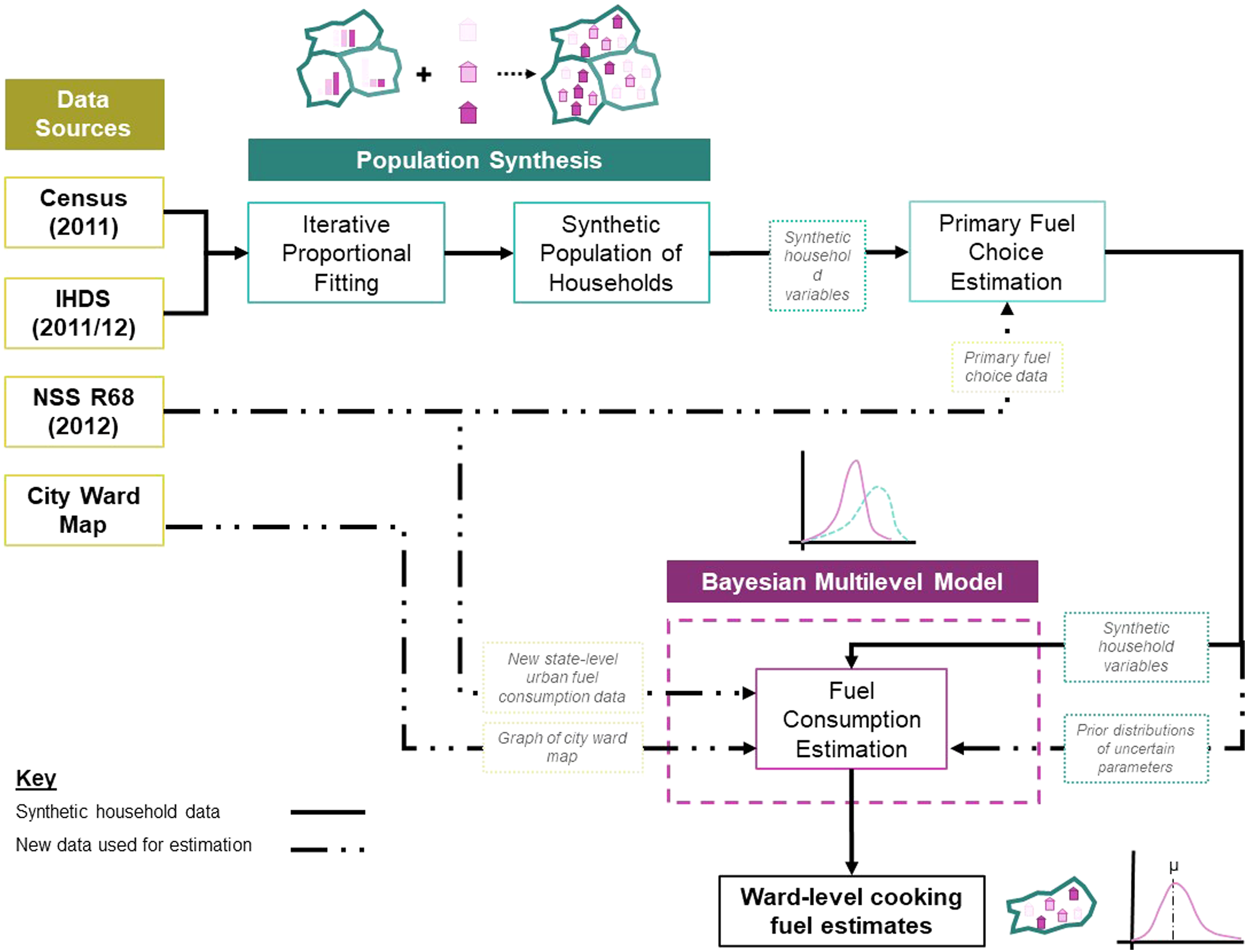

Microsimulation modelling naturally embodies uncertainties in the estimation of the synthetic population. These are challenging to quantify methodologically. The absence of test data generally renders any form of uncertainty management of the model parameters impossible. However, this approach will include and propagate the uncertainties arising from the variation across households in the dataset used for generating the synthetic population. As such, these represent the first order uncertainties, or the heterogeneity across similar clusters of households. The advantage of including these in the analysis is twofold: First, it helps understand the variability of outputs across different population groups; and second, it enables calibration of parameters as and when new data becomes available.

Data

The household-level data from the Indian Human Development Survey 2011 (IHDS-II) (Desai and Vanneman, 2015) and the 2011 census (Government of India, 2011) ward-level tables of household asset ownership are used to generate the synthetic population. Maps of the Census 2011 ward boundaries and National Sample Survey consumer survey data from Round 68 (National Sample Survey Organisation, 2013) are used as inputs for the multi-level model. The performance of the model is examined using survey data from 24 low-income wards across the four cities. Further details of the data sources including sample characteristics of ward-level survey data are detailed in the Data section in the Supplementary Material.

Household population synthesis

A synthetic population is generated using IPF (Lovelace and Dumont, 2016), a method also known as matrix raking, as introduced by (Deming and Stephan, 1940). This approach does have some drawbacks including reliance on categorical data, and ability to only control for household or individual-level attributes (Casati et al., 2015). However, this is well suited for this model given the data publicly available on Indian households, and that the household is the smallest unit of analysis not the individual. IPF offers the benefit of being computationally efficient, simple to use (including practical guidance on performing IPF in R (Lovelace and Dumont, 2016)) and converges to a single solution (Fienberg, 1970). The IHDS household-level data is used as the microdata consisting of a sample of representative individual urban households from the state. The census ward-level data is used as a contingency table of constraints to generate weightings for the individuals in the microdata. A detailed explanation of how IPF uses this data to generate a synthetic population, what assumptions are made and how weightings are integerised is detailed in Supplementary Figure 2 and Supplementary Tables S 1 and S 2 in the Supplementary Material.

Synthetic households are assigned to a primary cooking fuel group representative of current cooking practices. A categorical logistic regression of the form shown in equation (1) is used to infer the primary cooking fuel $j$ of a household $i$ based on the socio-economic characteristics of the household. The predictors used are household expenditure, majority religion membership, ration card possession, caste category and income frequency. These predictors were identified through exploratory analysis as having greatest relative importance out of available variables. The selected predictors include both income and non-income factors in line with previous research showing that non-income factors must also be considered in household fuel choice (Ahmad and Puppim De Oliveira, 2015; Sankhyayan and Dasgupta, 2019). The regression coefficients are estimated from the NSS data for the respective state. The household is assigned to one of six primary cooking fuel choice groups: No cooking, Biomass, Kerosene, Low LPG (uses less than a cylinder every month), High LPG (uses more than a cylinder every month) or Electricity. The primary cooking fuel choice groups are discussed in more detail in the Supplementary Material

j [i] = β_{0} + β_{1} {e x p}_{i} + β_{2} {r e l i g}_{i} + β_{3} {r a t i o n c a r d}_{i} + β_{4} {c a s t e}_{i} + β_{5} {i n c f r e q}_{i}

(1)

Generation and validation of the synthetic population for each of the four cities was done using base packages in R as well as the ‘ipfp’ package (Blocker, 2016).

Multi-level model specification

A multi-level model is used to estimate the magnitude of biomass and LPG use for each synthetic household on the basis of its socio-economic features and location. The model has three components which aim to address intrinsic features and practices of the household, extrinsic local socio-economic and cultural features, and spatial effects. The household-level component of the model uses an idealised linear relationship for the household’s mean fuel use with expenditure and household size (no. of persons) as predictors. These represent the intrinsic component of cooking fuel use, dependant on the features of the household. Coefficients for the household-level predictors are allowed to vary by primary cooking fuel group. This is a non-spatial and non-random group effect.

A novelty of this study is to quantify the influence of local socio-economic and cultural features on fuel use and access. These are extrinsic features which relate to the household’s interaction with its wider neighbourhood and community and spatial effects from its location within the city. Quantifying the impact of local features is complicated by the unmeasurable nature of some socio-cultural determinants of clean cooking access. This is addressed by adapting the approach of the Besag-York-Mollie model (Besag et al., 1991) used in spatial epidemiology studies (DiMaggio, 2015) which uses an Intrinsic Conditional Auto-Regressive (ICAR) to capture spatial effects and a random effects coefficient to capture extrinsic features. Similar approaches have been used in district-wise building energy use models (Choudhary and Tian, 2014), and recent studies have explored improved approaches for implementation (Morris et al., 2019).

The statistical model is shown in equation (2), where for a household $i$ in cooking fuel group $j$ and city ward $w$ fuel use is assumed to follow a normal distribution with a mean given by the sum of the household and ward-level components and with a precision $σ$ . In equation (2), $ϕ_{w [i]}$ is the ICAR component and $θ_{w [i]}$ is the random effects coefficient.

{f u e l}_{[i]} \sim N (a_{0 j [i]} + a_{1 j [i]} s i z e_{[i]} + a_{2 j [i]} e x p_{[i]} + ϕ_{w [i]} + θ_{w [i]}, σ)

(2)

Household-level predictor coefficients $a_{0}, a_{1},$ and $a_{2}$ are defined by the following parameters

a_{0 [i]} \sim N (μ_{a 0}, σ_{a 0})

a_{1 [i]} \sim N (μ_{a 1}, σ_{a 1})

a_{2 [i]} \sim N (μ_{a 2}, σ_{a 2})

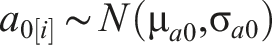
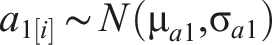
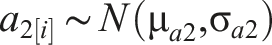
Parameters for the distributions of coefficients $a_{0}, a_{1},$ and $a_{2}$ are estimated from the NSS consumer survey data. A prior is set on the parameters using the fuel use values embedded in the synthetic population, which have been derived from the IHDS micro dataset. Four different versions of the model were implemented to compare the performance of the different components of the model. These four variants are a Basic Model which includes only household-level effects; a Random Effects Model which includes household-level predictors and the random effect coefficient; an ICAR Model which includes household-level predictors and an ICAR component; and a combined model which includes all three components (shown in equation (2)). Details of model variant formulations, priors and parameter definitions are detailed under Multi-level Model Variants in the Supplementary Material.

Models for each city are estimated separately, using NSS consumer survey data for the respective state. All expenditure and fuel consumption values are normalised and a square root transformation is also applied to fuel consumption values. Estimation of the parameters of the model is done using Stan which performs full Bayesian inference using Hamiltonian Monte Carlo. Stan’s No U-Turn Sampling (NUTS) performs better than alternative Gibbs or Metropolis algorithms for models with complex posteriors (Homan and Gelman, 2014). The RStan interface enables input and output data handling in R. It is important to note that as Gelman (2006) points out, multi-level models are advantageous for making predictions as they can estimate the effect of individual predictors as well as the group-level mean, but these cannot be necessarily interpreted as causal and this should be kept in mind when examining outputs.

Model performance

By comparing the model outputs to the survey data available for selected wards, the consistency of the model and its four variants can be examined. Figure 2 compares the model estimates for LPG and solid biomass use in each of the 24 wards included in the survey dataset. The points indicate the mean and lines show the 95% confidence interval of each model and the survey data ward-by-ward. The wards are ordered by their surveyed mean fuel consumption. Figure 2 shows that with a few exceptions, the survey means fall within the confidence interval for the combined model estimates, and in a majority of cases those of the random effects model too. Notice that the combined model estimates broadly follow the variation seen in the survey means with wards with lower survey means likely to have a lower model estimate than those with higher survey means. This is noteworthy as these wards were selected for the survey because of their low socio-economic status and greater likelihood to have lower access to LPG and use greater amounts of solid biomass; thus, they do not represent the full spectrum of wards but rather the lower end of LPG and upper end of solid biomass consumption.

Figure 2.

Comparison of model outputs and survey data for selected wards. Point values represent mean values from the model or survey samples, and lines indicate the 95% confidence interval.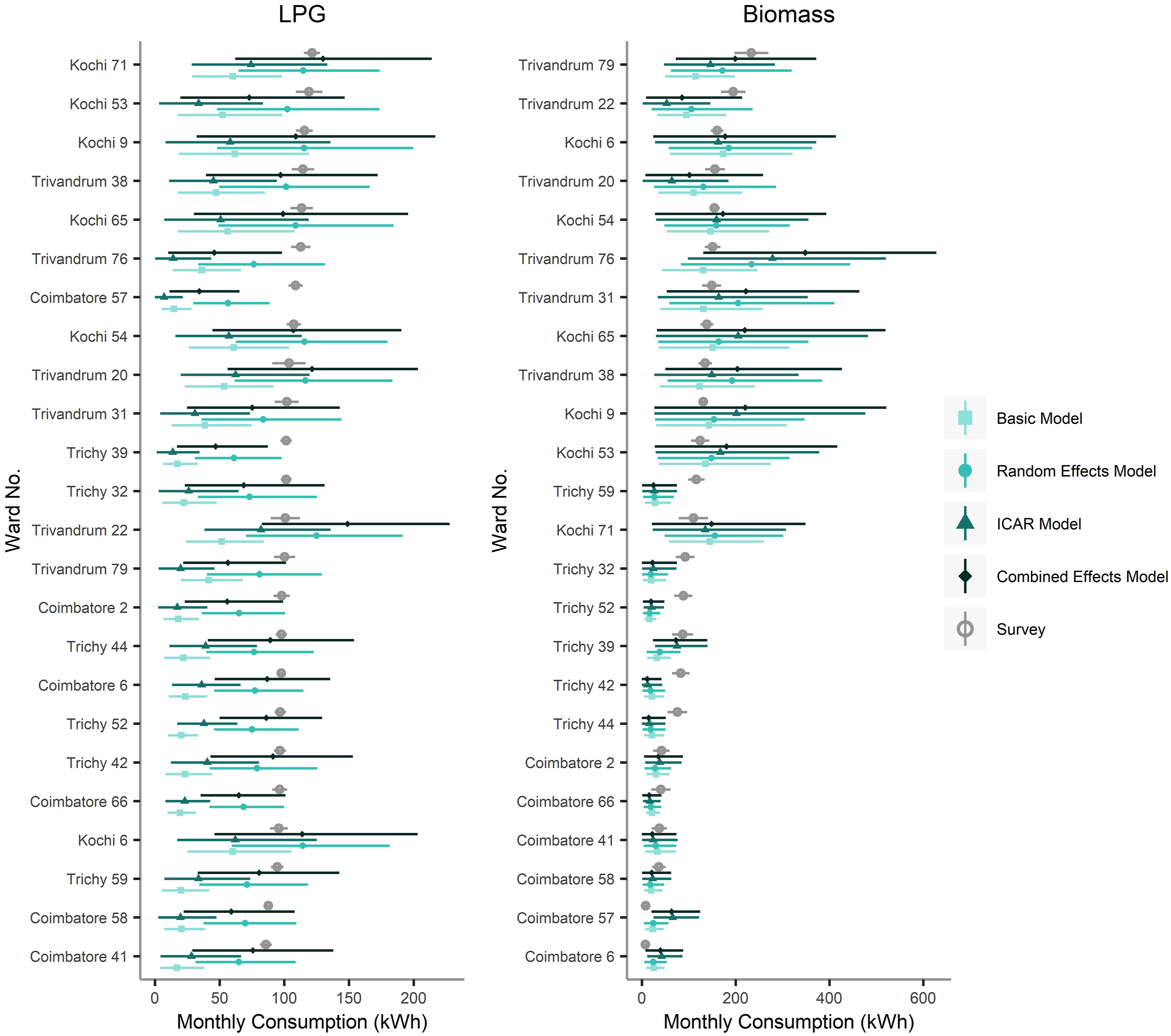

Comparing the different model variants, the basic model has the narrowest confidence intervals, and the interval increases for the random effects and ICAR models, with the combined model featuring the widest interval. This reflects the added uncertainty the estimates from these models account for. Recall that the basic model infers coefficients for predictors from NSS data on all urban households in the state, including those not in these cities. It represents the estimate of fuel use for that ward’s population of households assuming they are in an ‘average’ city in that state. The random effects model includes a coefficient that represents the impact of the ‘city effect’ versus the average city in the state. The ICAR model represents how the ward compares to the wards around it. Accounting for each of these effects adds uncertainty to the estimate and so the combined model has the widest confidence interval.

Model variant estimates differ in performance when compared to the survey data. For solid biomass consumption, there is little difference in the mean estimates between the four model variants, where the survey data means fall within the confidence interval of model outputs for most wards, particularly those with lower consumption levels. This indicates that the levels of consumption in each ward are similar to those in the average urban area in the state and that local spatial effects have a relatively modest effect on magnitude of consumption. The discrepancy between model estimates and survey data for some wards in Tiruchirappalli (abbreviated to Trichy in the figure) could represent a transient random effect, for example added use of fuel in the month surveyed due to a festival or greater availability of fuel.

The situation with LPG is rather different, where the basic model underestimates LPG use and the random effects and combined models are more compatible with the survey data. In this instance, the random effect coefficient provides the bulk of the adjustment from the basic model with the ICAR component adding only small additional adjustments. It is worth noting two points here; Firstly, the fact that these cities are larger than the average urban centre within their states would suggest that they are likely to have a better network of LPG suppliers than the average city. In addition, the survey data was collected in 2018–2019 coinciding with the government’s PMUY LPG connection initiative which targeted certain groups of low-income households, which possibly explains why in wards such as Coimbatore’s 57th or Trivandrum’s 76th the models underestimate LPG consumption.

Results & discussion

The focus of this microsimulation approach was to estimate spatial inequality in access and use of clean cooking fuels across cities, with the expectation that variation at a ward-level arises due to household context, local socio-economic and cultural factors and spatial effects. Examining the various components of the model is instructive to understand their influence on outputs and how uncertainty is propagated. At the heart of the basic model is a multi-level normal linear model whose coefficients vary according to the primary cooking fuel group a household is predicted to belong to. Figure 3 shows the estimated linear coefficients of the LPG consumption model for Tiruchirappalli across the six different primary cooking fuel groups. The prior is represented by the dotted line. Due to absence of a comparable primary cooking group variable in the raw synthetic population data the prior does not vary by group. Despite this limitation, using the synthetic population data to form a prior ensures consistency and makes for a reasonable prior.

Figure 3.

Linear coefficients of LPG household model by primary cooking fuel group for the city of Tiruchirappalli. LPG: liquified petroleum gas.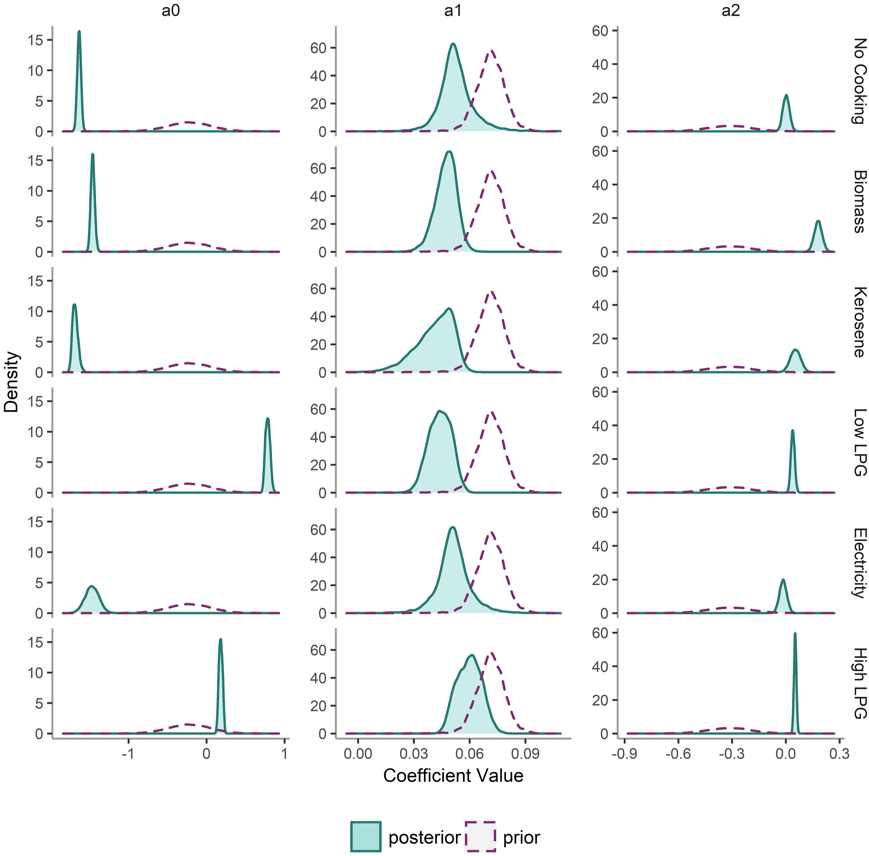

The new data from the NSS consumer survey helps reduce uncertainty in the model coefficients with posteriors having smaller variances. While all groups have the same prior, the new data and the model design allowing coefficients to vary by primary cooking fuel group greatly reduce uncertainty. For groups using kerosene and electricity as primary cooking fuels, some coefficient posteriors have greater variance than other groups. This is because in the case of Tiruchirappalli the NSS consumer survey data had considerably fewer instances of households in these two groups and there was variability in fuel use amongst these few cases. This resulted in posterior distributions for coefficients with slightly greater variance. Expenditure slope coefficient a2 for these groups shows uncertainty with respect to the positive or negative nature of this relationship, covering a range of values from approximately −0.05 to 0.15 for the kerosene group, and −0.1 to 0.1 for the electricity group. Interestingly, the coefficients for household size, coefficient a1 from equation (2), while having slightly different distributions between groups, have similar values within a range of 0.04–0.08, suggesting the effect of this predictor does not vary much with primary cooking fuel choice.

The components of the model that account for local socio-cultural features and spatial effects are the random effects and ICAR coefficients. These location-related coefficients offer valuable insight for the targeting of interventions as they quantify the impact of local socio-economic and community factors relative to the average ward in the state and in that city. The random effects coefficients across the city as a whole indicates whether the fuel consumption of that city is above, below or about average for the state. Figure 4 shows the distribution of estimated random effect coefficients across all wards in each of the four cities for both solid biomass and LPG consumption. They indicate all cities are highly likely to have a positive random effect coefficient for LPG with some small difference in magnitude between them, nonetheless, indicating LPG consumption above state urban area average. The same is not true for solid biomass consumption where, with the exception of Trivandrum, the random effect coefficient value for solid biomass consumption across the cities is normally distributed close to zero indicating that solid biomass consumption levels are close to the state urban average. Note the variance in the coefficient does vary slightly between cities and fuels, reflecting differences in uncertainty in the magnitude of difference between local fuel consumption compared to the state-wide average urban household.

Figure 4.

Distribution of random effects coefficients for both solid biomass and LPG across cities. LPG: liquified petroleum gas.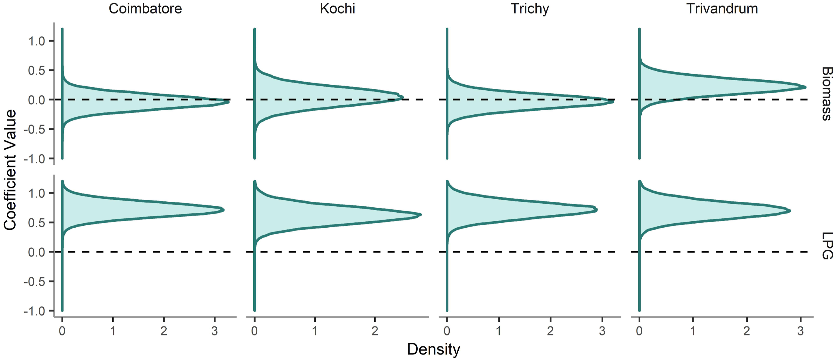

Figure 5 shows the mean ward-level random effects and spatial smoothing coefficients for LPG consumption across the city of Tiruchirappalli. The mean random effect coefficient shows negligible variation between wards and indicates that the city as a whole has a level of LPG use well above that of the average urban area in Tamil Nadu. Meanwhile the ICAR coefficient shows how city wards compare to each other. The central southern wards of the city have a positive coefficient indicating higher LPG use than the average ward, while the eastern wards underperform relative to the average ward. Analysis of the spatial distribution of ICAR coefficients provides a clear indication of which wards are below average in terms of uptake of LPG and may thus need additional targeted intervention.

Figure 5.

Ward-level random effects and ICAR coefficient values for Tiruchirappalli. ICAR: Intrinsic Conditional Auto-Regressive.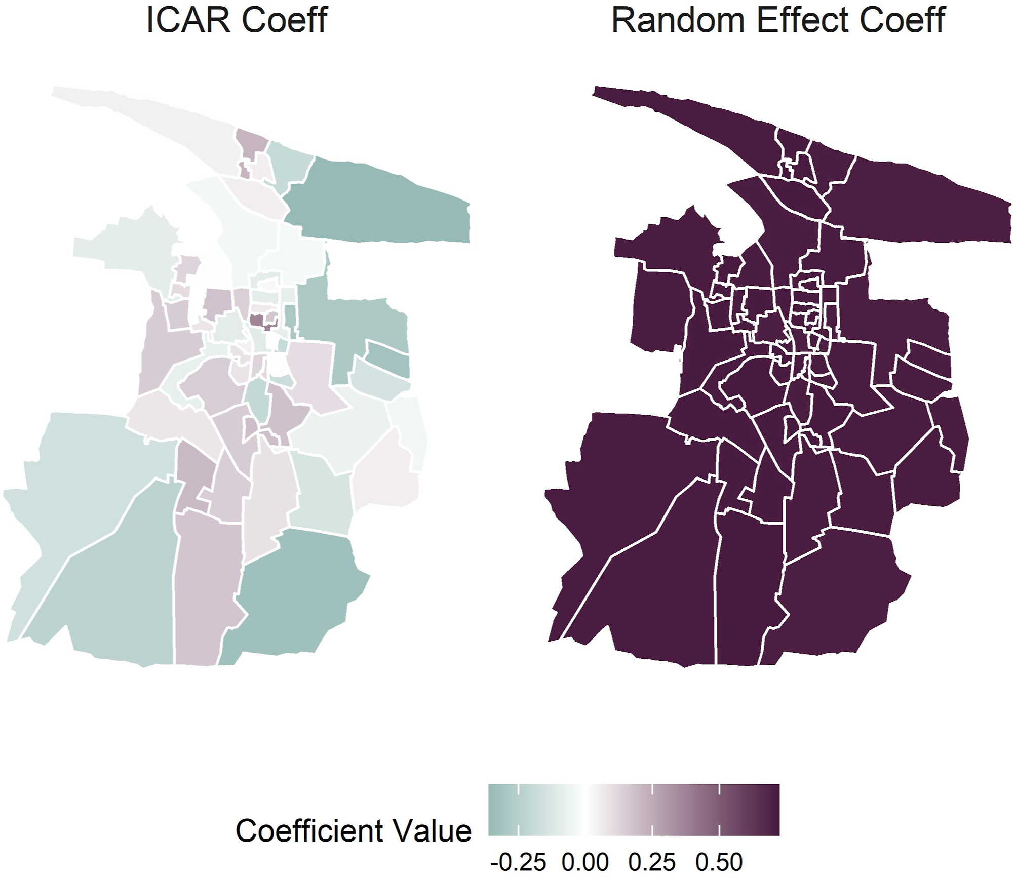

Putting these model components together they add up to produce the model fuel consumption estimates as shown in Figure 6, which illustrates the distribution of estimates of monthly LPG consumption for each of the four model variants in Ward 38 of Tiruchirappalli. The ICAR model indicates that ward 38 is likely to have above average LPG consumption compared to the city average, and the random effects model indicates that Tiruchirappalli’s LPG consumption is also likely to be above the state average. The contribution of these two coefficients is added to the basic model estimate in the combined model, resulting in a boost to the mean estimate. The uncertainty from the various individual components adds up with the ICAR and random effects models having greater variance than the basic model and this variance compounds in the combined model which accounts for the uncertainty in all three constituent model components.

Figure 6.

Distribution of LPG Consumption estimates for each of four model variants for Ward 38 in Tiruchirappalli. LPG: liquified petroleum gas.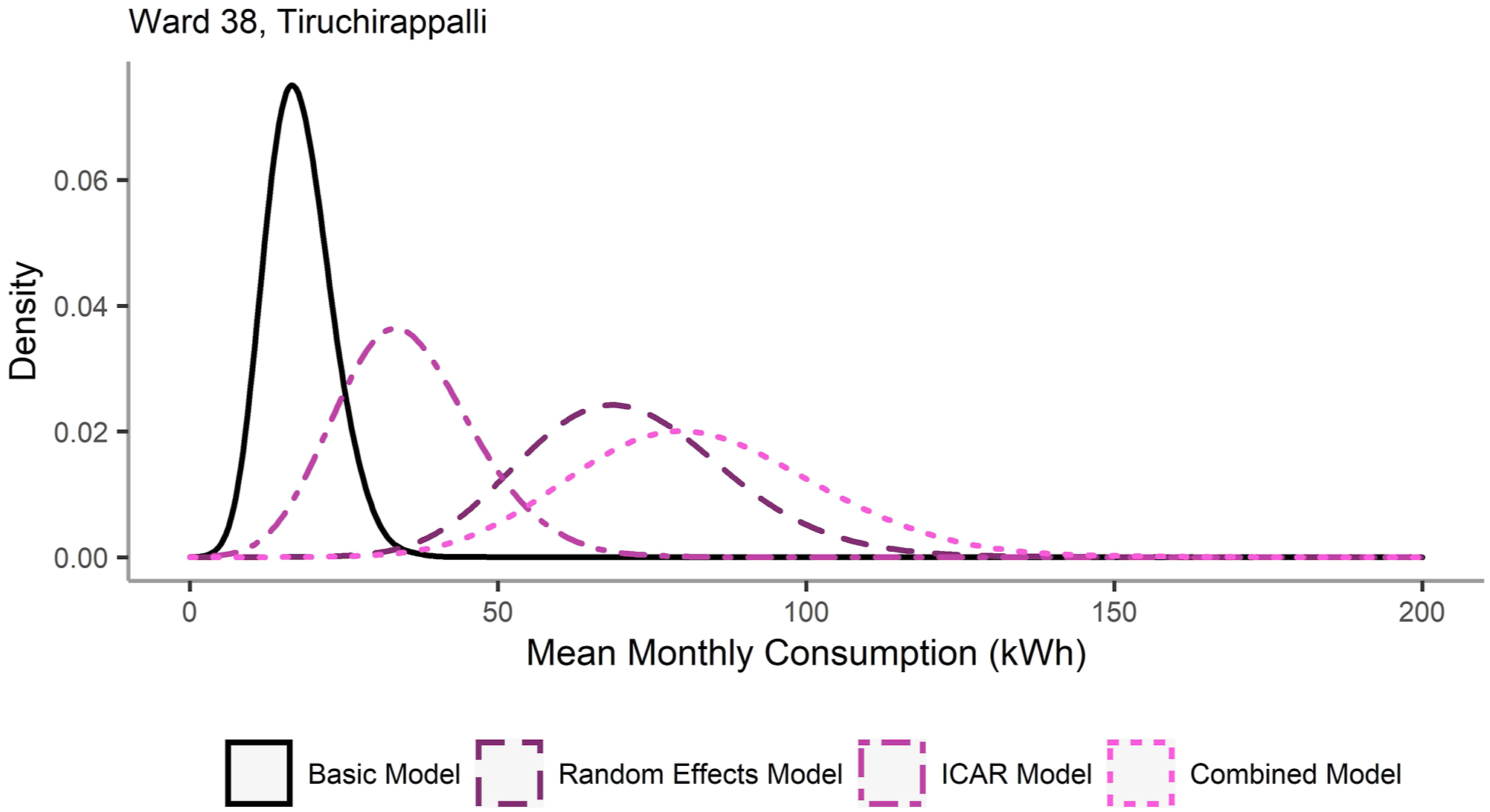

The impact of the different models is illustrated spatially in Figure 7, which shows the LPG consumption estimates across city wards for each of the four models. The estimates from the basic model show only small variation between wards while the random effects model boosts the estimates of fuel consumption relative to the basic model, although still preserving the relative homogeneity between wards. The spatial smoothing model introduces greater variation between wards with either an increased or decreased mean estimate compared to the base model. The combined model features both the city wide increase in mean estimated consumption while also including greater variation between wards, more fully capturing the spatial variability.

Figure 7.

Comparison of model variant estimates for mean monthly LPG consumption in Tiruchirappalli mapped by city wards. LPG: liquified petroleum gas.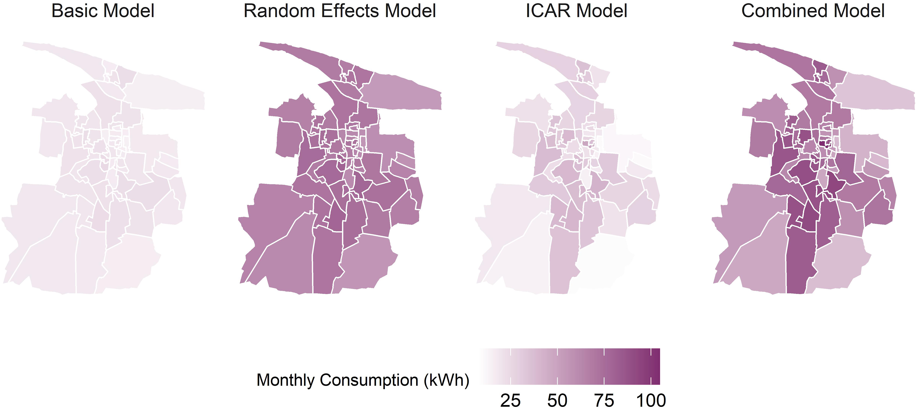

This approach can provide valuable insight for policy makers and stakeholders by locating wards most likely to have low sustained and exclusive clean cooking fuel use. The representative population of synthetic households offers an additional benefit by providing insight into ward-by-ward differences in socio-economic features that can contextualise model estimates. Figure 8 shows model estimates alongside socio-economic characteristics from the synthetic population in the southern edge of the city of Kochi, Kerala. Wards 47, 50, 51, 53 and 54 have lower levels of mean estimated LPG consumption than surrounding wards, although model outputs indicate that not all these wards with lower LPG consumption are equal. Amongst these, wards 47, 50 and 53 have a greater proportion of households with residual biomass use (continued biomass use in households with an LPG stove) suggesting that a different intervention may be required to encourage sustained and exclusive use of LPG in these wards. Some local socio-economic context is provided by the proportions of daily and weekly income earners by ward. Notice that many of the wards with high proportions of households paid daily or weekly are also those same wards with higher proportions of residual biomass users, such as wards 47 and 53. Similar outputs are mapped out in Supplementary Figures S.3, S.4 and S.5 for the other cities modelled.

Figure 8.

Model outputs for wards in south-eastern section of Kochi, Kerala. Outputs show mean LPG consumption, proportion of households with residual biomass use and households relying on daily/weekly income. LPG: liquified petroleum gas.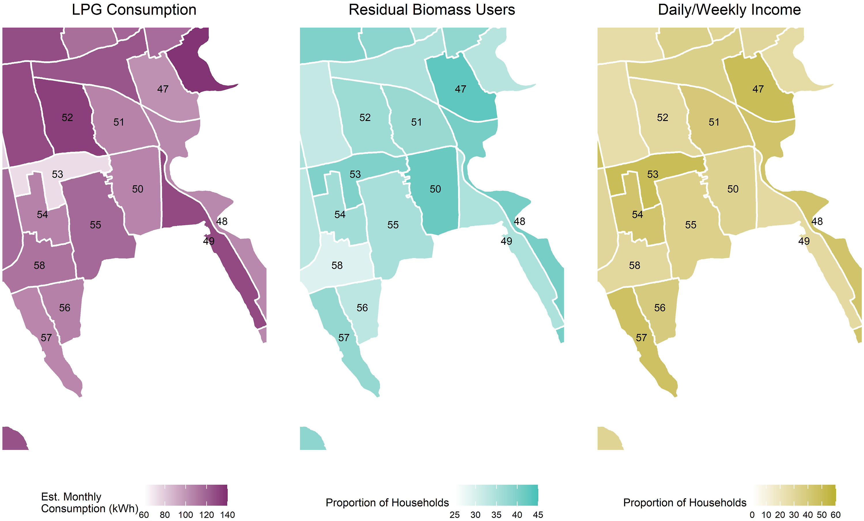

Interestingly, recent studies have shown how multi-level models can help identify and locate residential segregation in cities in the US (Arcaya et al., 2018) and UK (Jones et al., 2018). While the multi-level model microsimulation approach does not imply causality between variables it does contextualise spatial patterns and inequality in clean cooking access with local socio-economic factors. This can allow stakeholders to not only identify wards in need of further attention, but could provide a starting point for understanding the barriers and features of the transition pathways households in that ward may be following. Such data could also inform the setting of criteria for a particular policy or transition support initiative or even possibly support the local tailoring of such criteria for national policies.

There are obviously limitations to this approach some of which relate to the data used and model design. The ward-level aggregation may be too coarse for larger cities where wards have greater population density. Additionally the IHDS and NSS household-level data used may under represent some types of low-income and informal households. Furthermore the model is only as up to date as the data it uses, in this case that means the model is based on conditions in 2013. Inclusion of different types of data or new sources of data may offer a means to address some of these shortcomings and increase resolution and representation.

Conclusion

A microsimulation approach is proposed to estimate cooking fuel use across a city using publicly available data to help characterise spatial inequality in access to clean cooking. Using a multi-level model which accounts for household cooking practices, local city effects and spatial effects produced outputs that showed reasonable consistency with real world data. Allowing model parameters to vary by primary cooking fuel group reduced uncertainty in these, while the model structure propagated uncertainty in ward-level effects through to fuel use estimates. The random effect and spatial components capture the ‘city effect’ and ‘ward effect’ – the model offers insight into how fuel use in a given city compares to the average urban household in the state, and how the fuel use in a given city ward compares to the average fuel use in the city. By simulating a representative sample of households in each ward, spatial distribution of clean cooking access can be examined in context of socio-economic features across a city.

The results of this microsimulation have some important implications for current policy on clean cooking in India. The PMUY policy focuses on socio-economic indicators to target households; however, the findings from this study suggest that in cities some form of location-based targeting is also required. This could equate to different eligibility criteria for different urban areas. A second important implication for clean cooking policy is that spatial inequalities can lead to local barriers to access which may not be addressed by the current policy, for example areas within some wards may simply not be reliably serviced by a distributor. Identifying these areas and working closely with relevant stakeholders to address is necessary; in this example working with the distributor in the given area to ensure they reach out to all households.

More broadly the approach developed by this paper has potential to be deployed to model energy-related inequalities in other urban contexts. The use of national consumer surveys and census data to build the model makes this easy to implement in other countries as this type of data is quite commonly available. For example, inequalities in access to cooling will become more relevant as the effects of climate change lead to more frequent and intense heat waves. These would likely be exacerbated by urban heat island effects, modelling of which could be combined with the microsimulation approach in this paper to help anticipate vulnerable communities within cities.

With urban populations set to expand in the coming decades, limited data on the effects and distribution of urban spatial inequality is a challenge for policy implementation, not only for clean cooking, but wider energy access issues. Design of effective interventions requires stakeholder involvement and consideration of local household needs, and cost-effective modelling approaches such as the one proposed offer an exploratory view of clean cooking access across a city that can facilitate such a process.

Supplemental Material

sj-pdf-1-epb-10.1177_23998083211073140 – Supplemental Material for A microsimulation of spatial inequality in energy access: A bayesian multi-level modelling approach for urban India

Supplemental Material, sj-pdf-1-epb-10.1177_23998083211073140 for A microsimulation of spatial inequality in energy access: A bayesian multi-level modelling approach for urban India by André P Neto-Bradley, Ruchi Choudhary and Peter Challenor in Environment and Planning B: Urban Analytics and City Science

Footnotes

Acknowledgements

A.P. Neto-Bradley is grateful to the EPSRC for support through the CDT in Future Infrastructure and Built Environment (EP/L016095/1). This work was also supported by AI for Science and Government (ASG), UKRI’s Strategic Priorities Fund awarded to the Alan Turing Institute, UK (EP/T001569/1) and the Lloyd’s Register Foundation programme on Data-centric Engineering. The authors are grateful to Luke Archer at the Leeds Institute for Data Analytics, University of Leeds, for advice on generating synthetic populations using R. The authors would like to thank the Indian Institute for Human Settlements for assistance with shapefiles.

Declaration of conflicting interests

The author(s) declared no potential conflicts of interest with respect to the research, authorship, and/or publication of this article.

Funding

The author(s) disclosed receipt of the following financial support for the research, authorship, and/or publication of this article: This work was supported by the Engineering and Physical Sciences Research Council.

Data availability

All public data sources used can be accessed via the URL in the respective reference. Additionally some survey data was collected for comparison with model outputs. An anonymised version of this data is available at https://doi.org/10.17863/CAM.66449. Code for the model can be found at .

ORCID iD

André Paul Neto-Bradley

Supplemental Material

Supplemental material for this article is available online.

References

Ahmad

Puppim de Oliveira

(2015) Fuel switching in slum and non-slum households in urban India. Journal of Cleaner Production 94: 130–136. DOI: 10.1016/j.jclepro.2015.01.072.

Arcaya

Schwartz

Subramanian

(2018) A multi-level modeling approach to understanding residential segregation in the United States. Environment and Planning B: Urban Analytics and City Science 45(6): 1090–1105. DOI: 10.1177/2399808318760858.

Besag

York

Mollié

(1991) Bayesian image restoration, with two applications in spatial statistics. Annals of the Institute of Statistical Mathematics 43(1): 1–20. DOI: 10.1007/BF00116466.

Bhan

Jana

(2015) Reading spatial inequality in urban India. Economic and Political Weekly I(22): 49–54.

Bisaga

Parikh

(2018) To climb or not to climb? Investigating energy use behaviour among solar home system adopters through energy ladder and social practice lens. Energy Research & Social Science 44: 293–303. DOI: 10.1016/j.erss.2018.05.019.

Blocker

(2016) ipfp: fast implementation of the iterative proportional fitting procedure in C. Available at: https://CRAN.R-project.org/package=ipfp

Booth

Choudhary

Spiegelhalter

(2012) Handling uncertainty in housing stock models. Building and Environment 48: 35–47. DOI: 10.1016/j.buildenv.2011.08.016.

Casati

Müller

Fourie

, et al. (2015) Synthetic population generation by combining a hierarchical, simulation-based approach with reweighting by generalized raking. Transportation Research Record: Journal of the Transportation Research Board 2493: 107–116. DOI: 10.3141/2493-12.

Choudhary

Tian

(2014) Influence of district features on energy consumption in non-domestic buildings. Building Research & Information 42(1): 32–46. DOI: 10.1080/09613218.2014.832559.

10.

Deming

Stephan

(1940) On a least squares adjustment of a sampled frequency table when the expected marginal totals are known. The Annals of Mathematical Statistics 11(4): 427–444.

11.

Desai

Vanneman

(2015) India Human Development Survey-II (IHDS-II), 2011-12: Version 6. Inter-University Consortium for Political and Social Research. DOI: 10.3886/ICPSR36151.V6.

12.

DiMaggio

(2015) Small-Area spatiotemporal analysis of pedestrian and bicyclist injuries in New York City. Epidemiology 26(2): 247–254. DOI: 10.1097/EDE.0000000000000222.

13.

Ekholm

Krey

Pachauri

, et al. (2010) Determinants of household energy consumption in India. Energy Policy 38(10): 5696–5707. DOI: 10.1016/j.enpol.2010.05.017.

14.

Farsi

Filippini

Pachauri

(2007) Fuel choices in urban Indian households. Environment and Development Economics 12(6): 757–774. DOI: 10.1017/S1355770X07003932.

15.

Fienberg

(1970) An iterative procedure for estimation in contingency tables. The Annals of Mathematical Statistics 41(3): 907–917.

16.

Frayssinet

Merlier

Kuznik

, et al. (2018) Modeling the heating and cooling energy demand of urban buildings at city scale. Renewable and Sustainable Energy Reviews 81: 2318–2327. DOI: 10.1016/j.rser.2017.06.040.

17.

Gelman

(2006) Multilevel (hierarchical) modeling: what it can and cannot do. Technometrics 48(3): 432–435. DOI: 10.1198/004017005000000661.

18.

Government of India (2011) Census of India, census of India: office of the registrar general & census commissioner. Available at: https://censusindia.gov (accessed on 7 December 2018).

19.

Homan

Gelman

(2014) The No-U-turn sampler: adaptively setting path lengths in hamiltonian monte carlo. The Journal of Machine Learning Research 15(1): 1593–1623.

20.

International Energy Agency (2020a) Access to clean cooking – SDG7: Data and Projections – Analysis, International Energy Agency. Available at: https://www.iea.org/reports/sdg7-data-and-projections/access-to-clean-cooking (accessed on 8 January 2021).

21.

International Energy Agency (2020b) India 2020 - Energy Policy Review. Policy Review. Paris: International Energy Agency, p. 305.

22.

Jones

Manley

Johnston

, et al. (2018) Modelling residential segregation as unevenness and clustering: a multilevel modelling approach incorporating spatial dependence and tackling the MAUP. Environment and Planning B: Urban Analytics and City Science 45(6): 1122–1141. DOI: 10.1177/2399808318782703.

23.

Kemmler

(2007) Factors influencing household access to electricity in India. Energy for Sustainable Development 11(4): 13–20. DOI: 10.1016/S0973-0826(08)60405-6.

24.

Khosla

Sircar

Bhardwaj

(2019) Energy demand transitions and climate mitigation in low-income urban households in India. Environmental Research Letters 14(9): 095008. DOI: 10.1088/1748-9326/ab3760.

25.

Knight

Wells

Marshall

, et al. (2017) Developing a synthetic national population to investigate the impact of different cardiovascular disease risk management strategies: a derivation and validation study. Plos One 12(4): e0173170. DOI: 10.1371/journal.pone.0173170.

26.

Lovelace

Dumont

(2016) Spatial Microsimulation with R. Available at: https://spatial-microsim-book.robinlovelace.net (accessed on 3 July 2020).

27.

Morris

Wheeler-Martin

Simpson

, et al. (2019) Bayesian hierarchical spatial models: Implementing the Besag York Mollié model in stan. Spatial and Spatio-Temporal Epidemiology 31: 100301. DOI: 10.1016/j.sste.2019.100301.

28.

National Sample Survey Organisation (2013) India - household consumer expenditure, type 1 : july 2011 - june 2012, nss 68th round’. ministry of statistics & programme implementation, govenment of India. Available at http://microdata.gov.in/nada43/index.php/catalog/1 (accessed on 8 July 2020).

29.

Neto-Bradley

Rangarajan

Choudhary

, et al. (2021) A clustering approach to clean cooking transition pathways for low-income households in Bangalore. Sustainable Cities and Society 66: 102697. DOI: 10.1016/j.scs.2020.102697.

30.

Neto-Bradley

Choudhary

Bazaz

(2020) Slipping through the net: can data science approaches help target clean cooking policy interventions? Energy Policy 144: 111650. DOI: 10.1016/j.enpol.2020.111650.

31.

Nochta

Wan

Schooling

, et al. (2020) A socio-technical perspective on urban analytics: the case of city-scale digital twins. Journal of Urban Technology 28(0): 263–287. DOI: 10.1080/10630732.2020.1798177.

32.

Pandey

, (2021) Health and economic impact of air pollution in the states of India: the global burden of disease study 2019. The Lancet Planetary Health 5(1): e25–e38. DOI: 10.1016/S2542-5196(20)30298-9.

33.

Sankhyayan

Dasgupta

(2019) ‘Availability’ and/or ‘affordability’:what matters in household energy access in India?. Energy Policy 131: 131–143. DOI: 10.1016/j.enpol.2019.04.019.

34.

Sehjpal

Ramji

Soni

, et al. (2014) Going beyond incomes: dimensions of cooking energy transitions in rural India. Energy 68: 470–477. DOI: 10.1016/j.energy.2014.01.071.

35.

Tirumalachetty

Kockelman

Nichols

(2013) Forecasting greenhouse gas emissions from urban regions: microsimulation of land use and transport patterns in Austin, Texas. Journal of Transport Geography 33: 220–229. DOI: 10.1016/j.jtrangeo.2013.08.002.

36.

Zakhary

Rosser

Siebers

P-O

, et al. (2020) Using unsupervised learning to partition 3D city scenes for distributed building energy microsimulation. Environment and Planning B: Urban Analytics and City Science 48: 1198–1212. DOI: 10.1177/2399808320914313.

37.

Zhang

Robinson

Guhathakurta

, et al. (2018) Estimating residential energy consumption in metropolitan areas: a microsimulation approach. Energy 155: 162–173. DOI: 10.1016/j.energy.2018.04.161.

Supplementary Material

Please find the following supplemental material available below.

For Open Access articles published under a Creative Commons License, all supplemental material carries the same license as the article it is associated with.

For non-Open Access articles published, all supplemental material carries a non-exclusive license, and permission requests for re-use of supplemental material or any part of supplemental material shall be sent directly to the copyright owner as specified in the copyright notice associated with the article.

0.00 MB

0.55 MB