Sage Journals: Discover world-class research

Abstract

Although social scientists have long been interested in the effects of occupational gender composition on workers, previous research has rarely examined how working in a gender-atypical occupation affects people’s private lives. This study draws on 17 rounds of data from the National Longitudinal Survey of Youth 1997 to investigate how individuals in occupations with varying gender ratios differ in the stability of their intimate unions. The authors also consider various mechanisms that may explain the link between working in a gender-atypical occupation and union instability. Results from random-effects event-history models show that both men and women in gender-atypical occupations experience faster paces of union dissolution than their counterparts in gender-balanced or gender-typical occupations. Female-dominant occupations’ lower pay accounts for a modest portion of the effect of working in female-typed occupations on men’s union instability. By contrast, the more irregular work schedules of male-typed occupations explain a substantial part of why women in such occupations have lower union stability. The remaining associations between occupational gender composition and union instability, we suggest, reflect the tendency for men and women in gender-atypical occupations to undergo greater psychological strain, which in turn increases the difficulty of maintaining intimate relationships.

Keywords

occupational gender segregation gender-atypical occupations union dissolution occupational characteristics and union instability

Occupational gender segregation is one of the most persistent forms of gender disparity in the United States. Despite substantial growth in female educational attainment and labor force participation during the past half century (England 2010; Goldin 2014), men and women still mostly work in different occupational settings (Weeden, Newhart, and Gelbgiser 2018). As this segregation leads many occupations to be gender typed, scholars have devoted extensive attention to how working in female- or male-typed occupations affects men’s and women’s earnings, workplace authority, promotion prospects, working conditions, and perception of workplace culture (Budig 2002; England et al. 1988; Glass 1990; Kilbourne et al. 1994; Stier and Yaish 2014; Taylor 2010; Williams 1992, 1995).

Although existing studies tell us much about the effects of occupational gender composition on workers’ labor market outcomes, few researchers have asked how working in male- or female-typed occupations affects workers’ personal lives (McClintock 2020). Because job demands and the identity and strain derived from work may spill over into workers’ family and personal lives (Inanc 2018; Kelly et al. 2014; Mennino, Rubin, and Brayfield 2005; Moen et al. 2016), working in gender-atypical occupations—that is, occupations with larger shares of the other sex—should have implications for intrahousehold dynamics. Some recent research, for example, shows that the patterns of household division of labor for men and women in gender-atypical occupations differ from the patterns for those in other occupations (McClintock 2017; Schneider 2012), suggesting that occupational settings may influence how workers interact and negotiate with their intimate partners at home. If working in gender-atypical occupations indeed has a spillover effect on interactions with intimate partners, then it could also affect the quality and stability of workers’ marriages and other intimate unions. Moreover, the literature on union dissolution has long noted the importance of jobs and employment (Lyngstad and Jalovaara 2010). Higher levels of job stability and income, for example, prevent union dissolution for men (Blossfeld and Müller 2002; Doiron and Mendolia 2012; Poortman 2005). At the same time, jobs that are conducive to work-family conflict, such as those with rotation or nonstandard schedules, tend to increase union instability (Kalil, Ziol-Guest, and Levin Epstein 2010; Presser 2000). Because occupations with varying gender ratios differ in job demands, working conditions, and earnings and promotion prospects (Glass 1990; Kilbourne et al. 1994; Stier and Yaish 2014), and because individuals may be received differently in gender-atypical, as opposed to gender-typical, occupations (Kanter 1977a; Simpson 2005; Williams 1992), we may find occupational gender composition to be relevant to union stability as well.

In this study, we use data from the National Longitudinal Survey of Youth 1997 (NLSY97) to examine the relationship between working in gendered occupational settings and union stability for a contemporary cohort. Drawing from largely ethnographic evidence on social encounters of workers in gender-atypical jobs (e.g., Simpson 2004; Watts 2007; Williams 1995), we argue that the strain from working in occupations that are incongruent with one’s gender puts an extra burden on one’s intimate relationship, leading to greater union instability. At the same time, we investigate a series of alternative mechanisms, such as occupational differences in income and advancement opportunities, exposure to the other sex, required work effort, and schedule requirements, for the differing hazards of union dissolution among those in occupations with varying gender compositions. This analysis sheds light on both how and why occupational gender composition connects to union instability. By linking occupational gender composition to couple dynamics, this study also extends our knowledge of the potential consequences of the persistence of occupational gender segregation. Finally, by focusing on occupational gender composition, a job characteristic that previous research on union stability has largely overlooked,¹ this study enriches our understanding of the interface between individuals’ work and family lives.

Gender-Atypical Occupations, Job Strain, and Union Dissolution

Social scientists have been interested in how working in gender-atypical occupations affects people since Kanter’s (1977a, 1977b) classic work on “tokenism.” Kanter argued that women and men who constitute small minorities in their occupations or workplaces serve as tokens and thus become exceptionally visible. Enhanced visibility subjects such workers to greater performance pressure and scrutiny. With coworkers frequently distorting token workers’ attributes on the basis of gender stereotypes, women and men who serve as tokens in their occupations also likely face difficulty fitting in or avoiding gender-typed roles at work.

In Kanter’s theory, both men and women suffer from working in gender-atypical occupations. Later studies, however, indicate that men in customarily female occupations are not disadvantaged in earnings and promotions compared with women in the same occupations (Budig 2002; Cognard-Black 2004; Williams 1992). Conversely, women in male-dominant occupations are treated differently from their male peers, feel less supported at work, and ultimately more likely leave their occupations than women in other occupations (Glass et al. 2013; Maume 1999; Palmer and Lee 1990; Taylor 2010; Usui 2008). Various ethnographic studies further show that these women must make extra effort to adapt to their workplaces’ male-dominant cultures and gain acceptance (Dryburgh 1999; Miller 2004; Watts 2007). Consequently, women in occupations with high proportions of men are more likely than women in customarily female occupations to find their jobs unpleasant (Qian and Fan 2019).² Moreover, because women in male-dominant occupations internalize the low acceptance they face at work, they are more likely than men in their occupations to doubt their own career fit or professional expertise (Cech et al. 2011). All these day-to-day obstacles and challenges increase job strain, making it more emotionally draining for women to work in gender-atypical occupations.

Unlike women, men in gender-atypical occupations rarely report lower workplace support or find their jobs more unpleasant or meaningless compared with other men (Qian and Fan 2019; Taylor 2010). Even so, working in female-typed occupations may still raise psychological strain for men. The source of strain for men in customarily female occupations comes from the dissonance between their gender identity and their occupational choices (Henson and Rogers 2001; Simpson 2005). Previous research shows that these men are often compelled to defend their masculinity. Male librarians, teachers, and nurses, for example, tend to emphasize the less feminine aspects of their jobs, relabel the work to minimize its feminine connotation, and distance themselves from their female peers by gravitating toward different areas within their occupations (Simpson 2004; Snyder and Green 2008). In addition to the constant need to reduce the discomfort arising from the incongruence between their self-concept and their work identity, men in female-dominant occupations also must confront prejudice outside the workplace (Williams 1992, 1995). Because women’s work is generally devalued (Kilbourne et al. 1994), men in female-typed occupations are likely to be looked down on by their broader social networks and the general public. Such experiences can create additional strain.

Research on the work-family interface has long shown that job strain harms family life (Inanc 2018; Kelly et al. 2014; Mennino et al. 2005; Presser 2000). Stressful work-related experiences, such as job insecurity and schedule unpredictability, tend to accelerate union dissolution (Blossfeld and Müller 2002; Kalil et al. 2010; Poortman 2005; Presser 2000). Strain from working in gender-atypical occupations may similarly jeopardize intimate relationships and increase union instability. Not only should this strain hamper one’s ability to maintain a relationship, but those who are “gender deviant” in their market roles may also feel compelled to assert their gender identities more at home (Schneider 2012). That is to say, having a partner in a gender-atypical occupation may require both parties in a couple to put forth extra effort in their everyday interactions to offset the partner’s discomfort about gender identity. This additional requirement could further increase the difficulty for workers in gender-atypical occupations to have satisfying relationships. Thus, we expect:

Hypothesis 1: Both men and women in gender-atypical occupations will experience greater union instability than their counterparts in relatively gender-typical occupations.

If the strain that women in gender-atypical occupations experience is largely caused by the hostility and challenges they face in the workplace, then it may be aggravated as women spend more hours at work, consequently undermining their union stability. If the strain for men in female-dominant occupations results less from encounters in the workplace and more from conflict between their occupational choices and their gender identity, the same pattern may not apply to men. We therefore propose:

Hypothesis 2: Spending more hours working in gender-atypical occupations will increase union instability for women, but not men.

Alternative Pathways

Although we expect the strain from working in gender-atypical occupations to increase the difficulty of maintaining intimate unions, there are other pathways through which gender-atypical occupations may contribute to union instability. To argue that the job or role strain is the mechanism, we also need to test the validity of alternative explanations. Here we discuss alternative mechanisms and develop related hypotheses.

Required Work Effort

Human capital theory has long maintained that what drives men and women into different types of occupations is the effort the occupation requires (Becker 1985, 1991). The theory assumes that individuals’ effort is finite and that women expect to put considerable effort into childrearing and housework. Women are thus reluctant to pursue jobs that demand high levels of energy, leading to their different occupations from men’s.

The human capital account regarding work effort is not always tenable. Studies based on lab experiments and workers’ self-reported effort show that women actually put more effort into their paid work than men do (Bielby and Bielby 1988; Kmec and Gorman 2010), although some aspects of men’s jobs involve greater work intensity (Gorman and Kmec 2007; Roxburgh 1996). Regardless of whether women or men exert more effort at work, if male- and female-typed occupations indeed demand different levels of performance and energy, such differences could explain an association between occupational gender composition and union stability, because occupations that require extra effort may create greater conflict with workers’ family obligations. The effect of required work effort on union stability, however, may be weak for men, as their shares of housework and childcare are relatively small (Sayer 2005). Besides, men’s provider role may make their partners more willing to accommodate their need to expand additional energy at work. Thus, if the argument about effort is valid, we can expect:

Hypothesis 3: Taking into account required work effort will weaken the association between being in gender-atypical occupations and union instability, at least for women.

Economic Prospects

The importance of income and job prospects for union stability is well documented (Blossfeld and Müller 2002; Kalmijn, Loeve, and Manting 2007; Killewald 2016; Lyngstad and Jalovaara 2010). The traditional gender division of labor assigns men the role of provider for the family. Low economic prospects are likely to debilitate men’s ability to fulfill this role and thus weaken their union stability. By contrast, women gain greater economic independence from high income or promising careers, which makes it easier to exit an unhappy union (Kalmijn and Poortman 2006; Sayer and Bianchi 2000). Male-dominant occupations generally pay more and provide more opportunities for advancement than female-dominant occupations (Kilbourne et al. 1994; Mandel 2013). Thus, men in male-typed occupations may have lower hazards of union dissolution because of their occupations’ higher pay and better career prospects, whereas women in such occupations may have higher hazards for the same reason. This argument leads to:

Hypothesis 4: Taking into account earnings and job prospects will reduce the positive association between working in gender-atypical occupations and union instability.

Exposure

Working in gender-atypical occupations may also affect union stability because occupations serve as settings for men and women to meet potential partners (McClendon, Kuo, and Raley 2014). Gender-atypical occupations likely give workers greater exposure to members of the other sex. Previous researchers maintain that this exposure could contribute to divorce risk by creating opportunities for heterosexual men and women to form new relationships, but specific evidence on this mechanism is absent (McKinnish 2007; South, Trent, and Shen 2001).

Although systematic information on people’s exposure to romantic opportunities outside of their current unions is rarely available, we can derive and test related hypotheses from the exposure argument. If exposure is the mechanism linking occupational gender composition to union dissolution, workers in gender-atypical occupations should experience even greater union instability when their occupations offer more opportunities to socialize with others. After all, in occupations that require little interpersonal contact, such as statisticians and furniture finishers, the occupation’s gender composition is unlikely to affect workers’ chances of meeting the other sex. We therefore propose:

Hypothesis 5: Workers in gender-atypical occupations will experience especially greater union instability when their occupations require them to socialize with others more frequently.

If greater exposure to the other sex increases the chances of forming new relationships, making existing unions vulnerable, then the effect of this exposure should also be greater for those less committed to their current unions. Because marriages generally involve a higher level of commitment and are less likely to dissolve than cohabiting unions (Lyngstad and Jalovaara 2010), those in marriages should be less affected by exposure to potential partners. Thus, we can also derive the following hypothesis:

Hypothesis 6: Workers in gender-atypical occupations will experience even greater union instability when they are cohabiting rather than married.

Family Values

Another alternative reason why people in gender-atypical occupations may experience greater union instability is that they have different views about relationships and families from those in gender-typical occupations. Studies show that individuals with more traditional gender and family beliefs are less likely to experience union dissolution (Davis and Greenstein 2009; Kaufman 2000). Because workers in gender-atypical occupations, especially men, are thought to hold less traditional values (Lupton 2006), it is possible that their views about family make them less likely to stay in an intimate union when its quality is suboptimal, resulting in greater union instability. If this is the case, then we should expect the following:

Hypothesis 7: Taking into account the importance workers place on family will reduce the positive association between gender-atypical occupations and union instability.

Work Schedules

Male- and female-dominant occupations are also likely to differ in their scheduling demands. Previous research shows that one reason for the persistence of occupational gender segregation in the United States is that typically male occupations are more likely to require long working hours; such hours discourage women from entering male-dominant occupations (Cha 2013). Because spending very long hours at work tends to increase workers’ stress and lower their ability to balance work with family responsibilities (Wharton and Blair-Loy 2006), the different time demands of male- and female-dominant occupations could explain why women in gender-atypical occupations may experience greater union instability. Although working long hours can also increase work-family conflict for men, their socially prescribed provider role is likely to alleviate the impact of extended hours on union stability.

In addition to the amount of time spent at work, the ability to control work schedules is also important for work-family conflict and psychological well-being (Kelly et al. 2014; Moen et al. 2016). Because workers in occupations with less routine and predictable schedules tend to encounter more difficulty controlling their schedules, they may experience greater stress and work-family conflict, resulting in higher union instability. Whether customarily male or female occupations have more irregular schedules, however, is unclear. On one hand, retail and service occupations, many of which are female dominant, tend to have nonroutine schedules (Henly and Lambert 2014). On the other hand, quite a few male-dominant occupations involve outdoor work or travel and transportation (e.g., roofers, highway maintenance workers, freight inspectors, commercial pilots). Such occupations’ dependence on weather, distance, and other factors beyond individuals’ control makes their schedules irregular. Besides, a good number of female-typed occupations are confined in offices or institutions that have fixed operating hours (e.g., receptionists, office assistants, teachers), making it possible that male-dominant occupations, on average, have greater schedule irregularity. If this is the case, then schedule irregularity may also be a mechanism linking male-typed occupations with union instability for women. We can thus expect:

Hypothesis 8: Taking into account working hours and schedule irregularity will weaken the association between working in gender-atypical occupations and union instability for women.

Data

The data for this study come from rounds 1 to 17 of the NLSY97, which collects longitudinal information from a nationally representative sample of men and women born from 1980 to 1984. The NLSY97 has conducted interviews annually from 1997 to 2013 and biannually thereafter. The last round in our data was fielded in 2015–2016, when the respondents were in their mid-30s. By that time, 76 percent had reported marriages or cohabiting unions. Because the NSLY97 recorded the months and years when respondents experienced school enrollment, childbirth, intimate unions, and jobs, we are able to convert the data into person-month observations, with time-varying information for each respondent. For the information recorded yearly, such as respondents’ region, we create the person-month sample with the assumption that their information stayed the same from the current to the next interview.

Because our analysis focuses on the pace at which respondents’ intimate unions dissolve, the analytic sample includes only the person-months during which respondents were in cohabiting unions or marriages; they would not have been exposed to the risk for union dissolution when they were not married or cohabiting. For simplicity, we include both marriages and cohabiting unions in the same models while controlling for union type. An earlier exploration indicated that fitting the models separately for married and cohabiting unions did not affect the results in a meaningful way. We exclude intimate unions that began before respondents turned 16 years old, because unions formed at very young ages are likely to be qualitatively different. Because our main concern is how occupational characteristics are associated with union stability, we also eliminate observations with no valid information about respondents’ employment status or occupation. We further exclude person-months during which respondents reported being in a same-sex union, because some of the hypotheses, such as the ones derived from the exposure argument, would not apply to same-sex couples. Unfortunately, we are unable to make statistically meaningful comparisons between same- and different-sex union experiences because the former constitute only 1.2 percent of our person-month sample. Our final sample includes 247,746 person-months from 3,286 men and 310,133 person-months from 3,469 women.

Variables and Measurement

The statistical analysis addresses how the union stability of men and women in gender-atypical occupations differ from that of their peers in gender-balanced or gender-typical occupations. The dependent variable for the analysis is the dissolution of a union, coded 1 if respondents reported that their marriages or cohabiting unions ended in the observed month and 0 otherwise. To be certain about the time order, we use respondents’ characteristics at month t – 1 to predict their union ending in month t. For the main predictor of concern, we follow prior research and use the gender composition to measure the degree to which an occupation is gender atypical (e.g., Schneider 2012). Specifically, we use the occupational data reported in the 2000 census to construct a variable for the proportion of men in respondents’ occupations (range = 0–1). In an earlier analysis, we also tried measures of occupational gender composition that assume a nonlinear association with the dependent variable, but the results failed to support such an assumption.

We use data from the Occupational Information Network (O*NET) to measure various occupational characteristics relevant to the various alternative mechanisms discussed earlier, such as the occupation’s required work effort, sociability, and schedule regularity, as these variables are not available in the NLSY97. The O*NET is a database developed under the sponsorship of the U.S. Department of Labor for the sake of providing comprehensive information about different occupations. Data from O*NET version 20.1 are merged with the occupations reported in the NLSY97.

To measure occupations’ required effort, we create an index by averaging two O*NET items: (1) the extent to which achievement or effort is important to the performance of the job and (2) the extent to which taking initiative is important to the performance of the job (Cronbach’s α = .91). The values for both items range from 1 to 5, with 5 indicating the highest frequency. To test the hypothesis regarding economic prospects as a main pathway, we use the O*NET’s “occupational recognition,” a composite index created on the basis of the occupation’s likelihood for advancement, potential for leadership, and social prestige. We consider this index as a measure of occupations’ long-term prospects. Because income is also a critical component of economic prospects, we further introduce the job’s weekly compensation, including wages, bonuses, tips, and overtime pay. Here we use the specific compensation reported by the NSLY97 respondents for their jobs and take the natural logarithm of the compensation to reduce its skewedness. To avoid losing observations for missing values on compensation (4.4 percent), we also include a dummy variable for those who have jobs but do not report their total pay.

To examine the argument that gender-atypical occupations that facilitate more socializing opportunities expose workers to potential partners especially more, we construct an index of occupational sociability by averaging four O*NET items, all ranging from 1 to 5. The items are (1) the occupation’s requirement for face-to-face discussion, (2) the occupation’s demand for frequent contact with others, (3) the extent to which the occupation requires working with others on the job, and (4) the extent to which the occupation requires cooperation with others (Cronbach’s α = 0.79). We use the O*NET’s indicator of schedule irregularity for the hypothesis about work schedules. The O*NET use the question whether an occupation has (1) established, routine schedules; (2) irregular schedules that vary with weather conditions, production demands, and/or contract duration; or (3) seasonal schedules to assess schedule irregularity. Also related to work schedules, we include in the analysis the number of weekly hours that respondents reported on the job.

To test the hypothesis that the value placed on family explains any connection between working in gender-atypical occupations and union instability, we use two variables to indicate the extent to which respondents hold traditional family views. First, we measure family attitude using the NLSY97 question regarding how important respondents think it is to attend family events. Respondents were asked to choose “not at all important” (coded 0), “somewhat important” (coded 1), “fairly important” (coded 2), or “very important” (coded 3). Because the NLSY97 asked this question only in rounds 5, 7, 9, 11, 14, and 15, we assume that respondents held the same views from the time they provided responses to the question to the month before the next time they answered this question. Second, we introduce a measure of religiosity, which tends to be associated with traditional family attitudes, including promarriage and antidivorce views (Pearce and Thornton 2007). The NSLY97 asked how often respondents attended worship service from 2000 to 2011 and in 2015, with eight response categories ranging from “never” to “every day.” We code the variable from 1 to 8, with a higher value representing a higher level of religiosity. We similarly assume that respondents’ level of religious attendance stayed constant until the next time they answered the same question. For both the importance of family and religiosity, we use the mean value for the individual for the person-months where there is no valid information for the variable (e.g., person-months before respondents first answered the question) and introduce a binary indicator for missing values.

Other than the key predictors, we control for several time-varying individual and partner attributes. To start, we include in the models respondents’ levels of education (less than high school, high school, some college, university or more, or unknown). We also include a variable indicating whether respondents were in school (yes, no, or unreported) during the observed month, because previous research finds school enrollment to discourage union formation (Thornton, Axinn, and Teachman 1995). Next, we control for union type, namely, marriage versus cohabitation. Furthermore, we include a binary indicator for having a child three years old or younger. Our earlier analysis indicated children of this age group are the only ones relevant to union stability. An additional dummy variable is used for those missing information about childbearing histories. We also control for the age at which respondents entered the union, because entering an intimate union at a more mature age may increase the union’s stability. We further introduce the union partner’s education level (less than high school, high school, some college, university or more, or unreported) and employment status (employed, not employed, or status unreported).³ In addition, we use a dummy variable to indicate that respondents had broken up and reunited with the partner observed in the person-month. Because we consider an intermittent relationship as a single union episode, this indicator enables us to distinguish such a relationship, which should be at greater risk for dissolution, from a continuous one.

The models also contain controls related to respondents’ employment, including whether they held a job in the observed month, their work experience since age 14 (in weeks), and the length of tenure of their current jobs. All these characteristics may be relevant to both their types of occupations and family lives. Other controls include respondents’ geographic region (Northeast, North Central, West, and South) and whether they live in urban areas. For both variables we include a separate category for missing information. We further introduce three time-constant variables that are potentially related to union instability: race/ethnicity (non-Hispanic White, non-Hispanic Black, Hispanic, or other); class background, measured by their parents’ highest educational level; and the structure of the family when the respondent was 12 years old (intact two-parent family, single-mother household, stepparent family, other types, or unknown).⁴

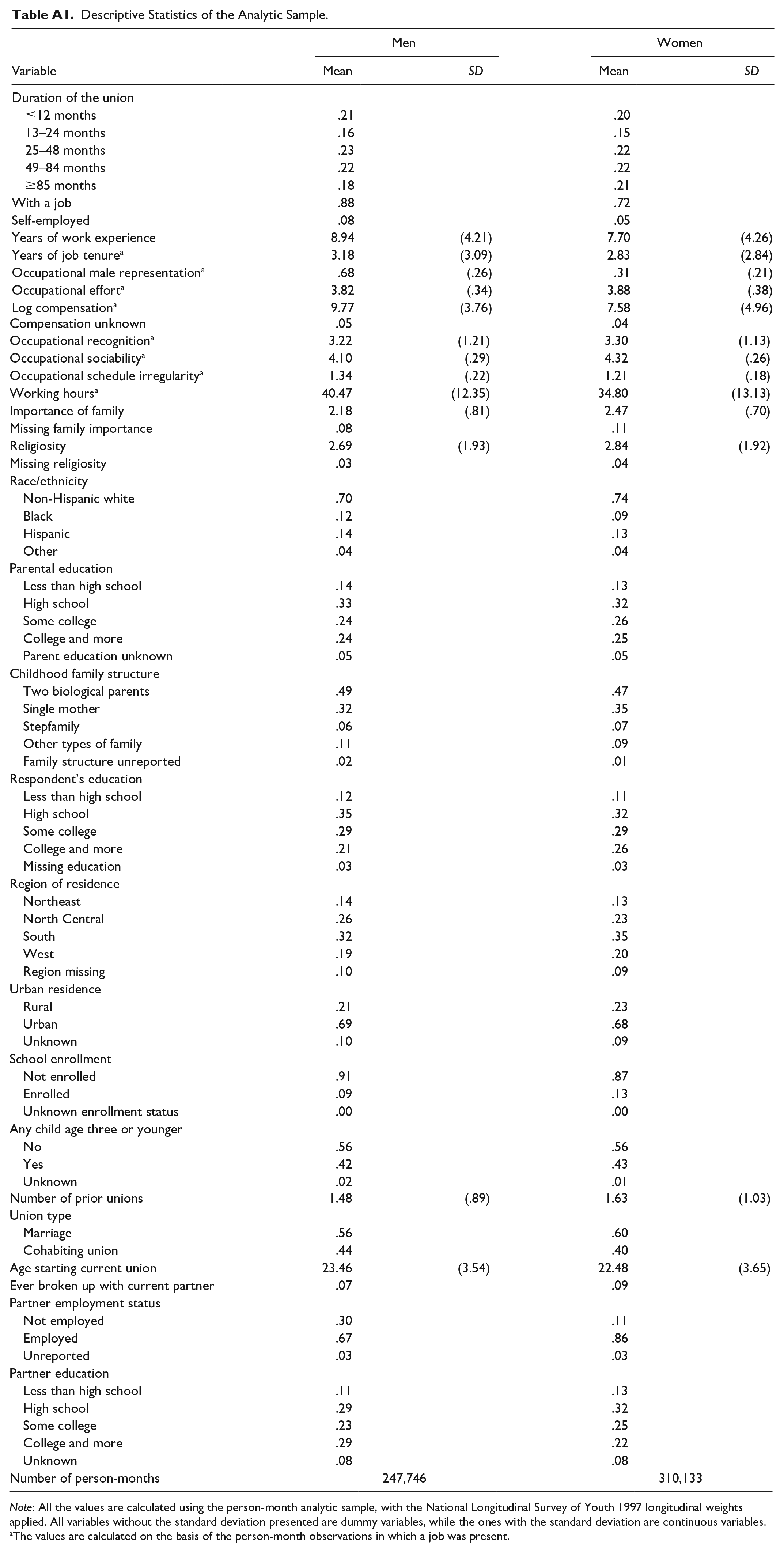
Because a respondent could have multiple union episodes in the sample time period, and the hazard of union dissolution may change as they experience more episodes, we control for the number of intimate unions reported before the current one in all models. To capture the time-dependent nature of the hazard of union dissolution, our models also include the duration of exposure (in months) to the hazard, which restarts with every new episode of each respondent (Yamaguchi 1991). On the basis of our earlier exploration, we divide the duration of exposure into five categories: (1) 0 to 12, (2) 13 to 24, (3) 25 to 48, (4) 49 to 84, and (5) 85 or more. Measuring the duration differently, for example by using a continuous measure, did not affect the results substantively. Table A1 in the Appendix provides descriptive statistics for all the variables.

Analytic Strategy

As in most studies of union stability (Kalmijn and Poortman 2006; Kalmijn et al. 2007; Poortman 2005), we use an event history approach to analyze the hazard of union dissolution. This approach enables us to examine how time-varying factors, such as occupational characteristics, are associated with the hazard of union dissolution, while taking into account cases that have not experienced a breakup of their unions (i.e., right-censored cases) (Yamaguchi 1991). Specifically, we use random-effects discrete-time logit models, which can be expressed as follows:

\ln [p_{i t + 1} / (1 - p_{i t + 1})] = γ_{0} + γ_{j} {Dur}_{j i t} + \sum α_{k} X_{k i t} + u_{i},

(1)

where p_it is the probability of an exit from an intimate union for the ith respondent at month t + 1, conditional on this union not ending earlier; γ₀ is the intercept; γ_j indicates the coefficients of the j dummies for duration of exposure to the risk for union dissolution; X_i represents k time-variant or time-constant covariates as described in the previous section, with Σα_k as their coefficients; and u_i is the individual-level random effect that is assumed to be normally distributed with a mean of zero and variance σ². The inclusion of an individual-level random effect in the models allows us to account for unobserved characteristics that are shared among observations from the same person (Steele, Goldstein, and Browne 2004). This strategy is suitable when a sizable portion of the observations are right censored (Chamberlain 1988; Wu 2003). It also helps us address the potential correlations of the multiple union episodes that the same individuals may have experienced during the observation period.

Because many of our key predictors are occupational characteristics, while our sample includes observations during which respondents had no job, we further transform equation 1 to the following to handle the variables whose values are conditional on respondents having jobs:

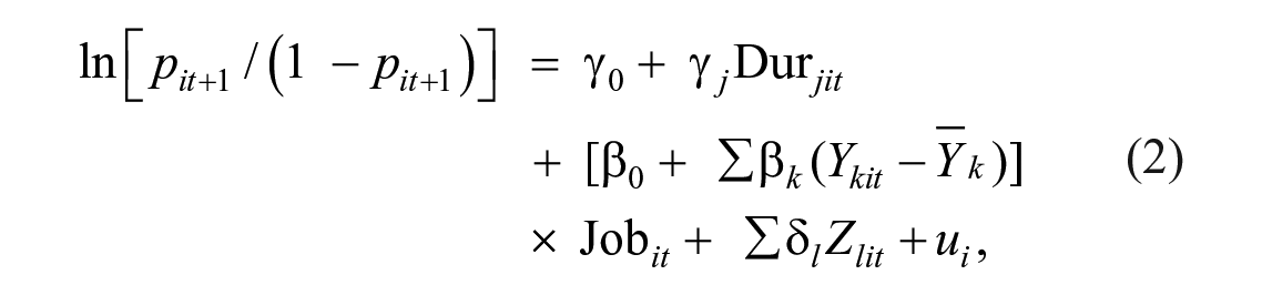
\begin{array}{l} \ln [p_{i t + 1} / (1 - p_{i t + 1})] = γ_{0} + γ_{j} {Dur}_{j i t} \\ + [β_{0} + \sum β_{k} (Y_{k i t} - {\bar{Y}}_{k})] \\ \times {Job}_{i t} + \sum δ_{l} Z_{l i t} + u_{i}, \end{array}

(2)

where Y_kit represents k job-related variables, which have values only when respondent i is employed at time t; $\bar{Y_{k}}$ indicates the average of each of the k variables; Σβ_k represents the coefficients for each unit of increase in the k variables from their respective average levels; Job_it is the ith respondent’s job status at time t, which takes the value of 1 if the respondent has a job and 0 if not; β₀ indicates the difference in the hazard of union dissolution between those with average values for Y_kit (i.e., average job characteristics) and those without a job; Z_lit represents l covariates of which the values do not depend on respondents’ job status (e.g., education, religiosity, attitude about the importance of family); and Σδ_l indicates the coefficients for such covariates.⁵

We fit the models separately by gender. Because the NLSY97 oversampled certain minority groups and had some attrition over time, we apply the survey’s longitudinal weights that are designed to address both issues and estimate robust standard errors for all models. Because discrete-time event-history models rely on logit regression techniques, they face difficulties similar to those associated with logit models with regard to the comparability of coefficients across models (Mood 2010). We therefore compare model fit with Wald tests to determine which covariates should be included in the final models. We also use the decomposition method proposed by Karlson, Holm, and Breen, known as the KHB method (Breen, Karlson, and Holm 2013; Kohler, Karlson, and Holm 2011), to more formally assess the extent to which a given covariate mediates or confounds the association between occupational gender composition and union instability.⁶ The KHB method makes the proper adjustments for the rescaling of nonlinear models and thus enables comparisons between coefficients across logit regression models. Nevertheless, because the KHB method is incompatible with weighted random-effects logit models, for the mediation analysis we remove the random effects from the models and simply compare coefficients across weighted logit models. Our additional analysis showed that the models yielded very similar results with and without the random effects. We thus feel comfortable about relaxing the random-effect assumption in the mediation analysis using the KHB method.

Results

Table 1 shows discrete-time hazard rate models predicting union dissolution for men and women. According to the table, men in occupations with higher proportions of men have lower odds of exiting a union. Specifically, a decrease of 30 percentage points from the average male share of the occupation contributes to a 10 percent increase in the odds of union dissolution each month (exp[–.3 × –.332] = 1.104). Conversely, women in occupations with larger shares of men have greater hazards of experiencing a union dissolution. An increase of 30 percentage points from the average male share of the occupation—roughly the change from a gender-balanced to a male-typed occupation—is associated with a nearly 10 percent increase in women’s odds of exiting a union in any given month (exp[.3 × .297] = 1.093). Thus, the results for both men and women support that working in a gender-atypical occupation accelerates union dissolution (hypothesis 1).

Table 1.

Random-Effects Discrete-Time Hazard Rate Models Predicting Union Dissolution.

	Men		Women
With a job	−.170**	(.064)	.100	(.053)
Self-employed	.152	(.083)	.001	(.108)
Years of work experience	−.033**	(.010)	−.020*	(.010)
Years of job tenure^a	−.033**	(.012)	−.065**	(.013)
Occupational male representation^a	−.332**	(.100)	.297**	(.108)
Race/ethnicity (reference: non-Hispanic white)
Non-Hispanic black	.030	(.058)	.200**	(.056)
Hispanic	−.130*	(.064)	−.124*	(.063)
Other	−.098	(.159)	.068	(.097)
Parental education (reference: less than high school)
High school	.061	(.063)	.050	(.073)
Some college	.026	(.072)	.184*	(.077)
College and more	.141	(.084)	.160	(.086)
Missing parent education	.032	(.119)	.066	(.103)
Childhood family structure (reference: intact two-parent family)
Single-mother family	.057	(.056)	.202**	(.051)
Stepparent family	.298**	(.099)	.285**	(.080)
Other	.112	(.082)	.295**	(.077)
Family structure unreported	−.334*	(.151)	−.084	(.172)
Respondent’s education (reference: high school)
Less than high school	.117	(.064)	.128	(.067)
Some college	.161*	(.076)	.122	(.074)
College or more	−.325*	(.127)	−.031	(.103)
Unknown	.074	(.134)	.026	(.118)
School enrollment (reference: not enrolled)
Enrolled	−.019	(.080)	.072	(.055)
Unknown enrollment status	.191	(.378)	.451	(.252)
Any child age three or younger (reference: no)
Yes	−.190**	(.047)	−.181**	(.043)
Unknown	−.142	(.139)	−.677	(.371)
Number of prior unions	.035	(.028)	.052*	(.023)
Union type (reference: marriage)
Cohabiting union	1.004**	(.060)	1.026**	(.057)
Age starting current union	−.049**	(.009)	−.048**	(.009)
Having broken up with current partner	.304**	(.082)	.162*	(.065)
Partner’s employment status (reference: not employed)
Employed	.033	(.049)	−.275**	(.051)
Unknown	−.070	(.082)	−.485**	(.080)
Partner’s education (reference: less than high school)
High school	.086	(.073)	−.084	(.065)
Some college	−.038	(.085)	−.347**	(.078)
College and more	−.488**	(.111)	−.655**	(.100)
Partner’s education unknown	1.554**	(.085)	1.459**	(.074)
Constant	−3.952**	(.224)	−4.171**	(.199)
Number of person-month observations	247,746		310,133

Note: Values in parentheses are robust standard errors. The National Longitudinal Survey of Youth 1997 longitudinal weights are applied to all models. The models also control for duration of exposure, region, and whether respondents lived in urban areas, but the coefficients are omitted to conserve space.

Variables are centered at the sample mean.

p < .05. **p < .01.

To examine the various mechanisms that may explain workers’ faster paces of union dissolution while working in gender-atypical occupations, we fit a series of models and compare the model fit using Wald tests.⁷ We build the models gradually and only add a variable when the Wald test indicates that the addition significantly improves the model. Table 2 presents coefficients from models for men, with the results for model comparisons included at the bottom of the table. In the model that addresses the argument about work effort, the inclusion of the occupation’s required effort significantly improves the model, but the coefficient for the male representation in the occupation hardly changes. Moreover, men in occupations requiring more effort are less likely to undergo a union dissolution, which contradicts the argument that greater work effort increases union instability.

Table 2.

Results From Random-Effects Discrete-Time Models Predicting Union Dissolution for Men.

	Explanation
	Work Effort	Economic Prospects		Exposure		Values		Schedules
	(1)	(2)	(3)	(4)	(5)	(6)	(7)	(8)
Union type (reference: marriage)
Cohabiting union	.997**	.992**	.994**	.992**	1.006**	.991**	.963**	.965**
Cohabiting union	(.060)	(.060)	(.060)	(.060)	(.072)	(.061)	(.062)	(.062)
Occupational male representation^a	−.346**	−.294**	−.294**	−.282*	−.229	−.293**	−.294**	−.235*
Occupational male representation^a	(.100)	(.100)	(.100)	(.114)	(.198)	(.100)	(.100)	(.112)
Occupational effort^a	−.174*	−.143	−.224*	−.152	−.142	−.143	−.141	−.147
Occupational effort^a	(.082)	(.083)	(.111)	(.089)	(.083)	(.083)	(.083)	(.083)
Log compensation^a		−.116**	−.119**	−.116**	−.116**	−.115**	−.116**	−.126**
Log compensation^a		(.032)	(.032)	(.032)	(.032)	(.032)	(.032)	(.038)
Compensation unknown		−1.423**	−1.459**	−1.427**	−1.425**	−1.421**	−1.429**	−1.531**
Compensation unknown		(.358)	(.358)	(.359)	(.359)	(.359)	(.361)	(.416)
Occupational recognition^a			.039
Occupational recognition^a			(.038)
Occupational sociability^a				.033
Occupational sociability^a				(.143)
Occupational male representation^a × sociability^a				−.025
Occupational male representation^a × sociability^a				(.422)
Occupational male representation^a × cohabiting					−.083
Occupational male representation^a × cohabiting					(.215)
Family importance						−.005
Family importance						(.027)
Missing family importance						.023
Missing family importance						(.068)
Religiosity							−.034*	−.034*
Religiosity							(.014)	(.014)
Missing religiosity							.032	.031
Missing religiosity							(.089)	(.089)
Occupational schedule irregularity^a								−.161
Occupational schedule irregularity^a								(.140)
Working hours^a								.001
Working hours^a								(.002)
Constant	−3.957**	−3.990**	−3.986**	−4.006**	−3.989**	−4.012**	−3.886**	−3.886**
Constant	(.225)	(.225)	(.224)	(.229)	(.225)	(.249)	(.242)	(.242)
Number of person-months	247,746	247,746	247,746	247,746	247,746	247,746	247,746	247,746
Model comparison	vs. baseline	vs. (1)	vs. (2)	vs. (2)	vs. (2)	vs. (2)	vs. (2)	vs. (7)
Change in df	1	2	1	1	2	2	2	2
χ²	4.50*	16.61**	1.04	.15	.06	.14	6.15*	1.49

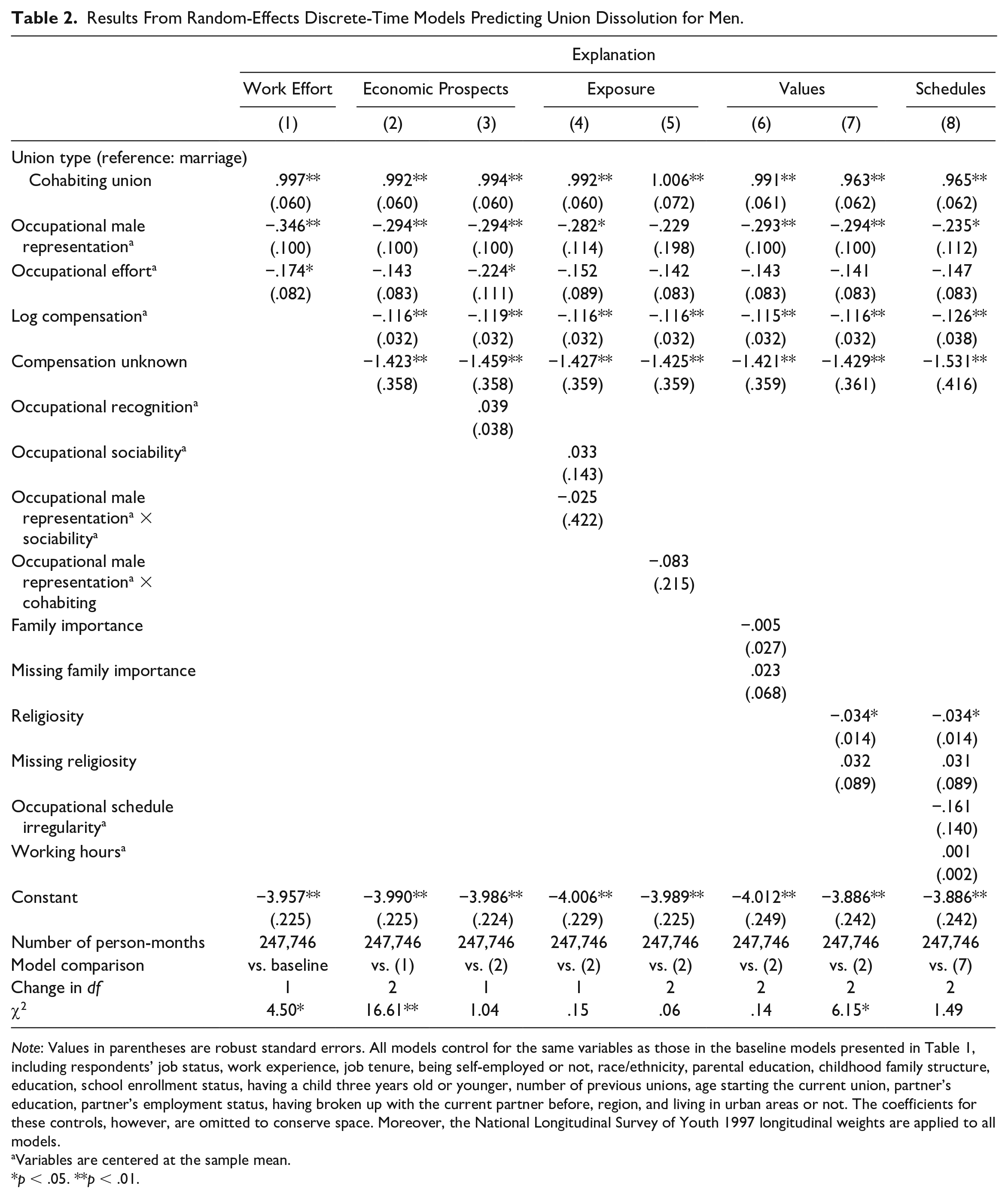
Note: Values in parentheses are robust standard errors. All models control for the same variables as those in the baseline models presented in Table 1, including respondents’ job status, work experience, job tenure, being self-employed or not, race/ethnicity, parental education, childhood family structure, education, school enrollment status, having a child three years old or younger, number of previous unions, age starting the current union, partner’s education, partner’s employment status, having broken up with the current partner before, region, and living in urban areas or not. The coefficients for these controls, however, are omitted to conserve space. Moreover, the National Longitudinal Survey of Youth 1997 longitudinal weights are applied to all models.

Variables are centered at the sample mean.

p < .05. **p < .01.

The next set of models, which tests the hypothesis about economic prospects, indicates that men with higher job compensation have lower odds of exiting an intimate union, but those in occupations that promise more advancement and recognition are no different from others in their union stability. Adding financial compensation also significantly improves the model. Models 4 and 5 test the hypotheses related to how working in gender-atypical occupations may expose heterosexual individuals to more members of the other sex. Contrary to hypothesis 5, we find no significant effect for the interaction between occupational male representation and sociability. Men in female-typed occupations are no more likely to exit a union when their occupations also provide more socializing opportunities. Similarly, the added interaction between occupational male representation and union type in model 5 neither improves the model nor supports the exposure mechanism. Men working in gender-atypical occupations are not significantly more likely to exit a cohabiting union than a marriage, which rejects hypothesis 6.

Models 6 and 7 in Table 2 examine the mechanism about family-related values. The expressed importance of the family is not significantly associated with union stability for men. Those who are more religious, however, have lower odds of union dissolution during a given month. Although the relationship between religiosity and union instability is as expected, the coefficient of occupational male representation changes little when religiosity is included in the model. Model 8 tests whether work schedules could be a mechanism linking occupational gender composition to union stability. We find that neither hours spent on the job nor irregular schedules of the occupation significantly affect men’s hazards of union dissolution. As argued earlier, because men’s socially prescribed family roles do not require them to spend as much time as women on childrearing and housework, it is possible that work schedules only matter for women, not for men.

Table 3 shows random-effects discrete-time models predicting union dissolution for women. Model 1 indicates that adding required work effort for the occupation significantly improves the baseline model shown in Table 1. Like their male counterparts, women in occupations that require greater than average effort have lower odds of exiting their intimate unions during a given month, which clearly contradicts the argument that a higher level of required work effort increases union instability. Furthermore, the inclusion of required work effort does not appear to weaken, but rather somewhat amplifies, the effect of occupational male representation. Models 2 and 3 demonstrate that neither monetary compensation nor the occupation’s prospects for advancement and recognition are significantly linked to women’s odds of union dissolution. These results reject the hypothesis that the better economic prospects in male-typed occupations account for the association between these occupations and women’s union instability. Although job compensation is not significantly associated with the hazard of union dissolution for women, the Wald test indicates that including it and the dummy for missing compensation significantly improves the model fit. We therefore include these variables in the remaining models.

Table 3.

Results from Random-Effects Discrete-Time Models Predicting Union Dissolution for Women.

	Explanation
	Work Effort	Economic Prospects		Exposure		Values		Schedules
	(1)	(2)	(3)	(4)	(5)	(6)	(7)	(8)
Union type (reference: marriage)
Cohabiting union	1.021**	1.021**	1.021**	1.023**	.975**	1.019**	1.012**	1.019**
Cohabiting union	(.057)	(.056)	(.056)	(.056)	(.061)	(.057)	(.057)	(.056)
Occupational male representation^a	.313**	.312**	.315**	.251*	.636**	.309**	.309**	.157
Occupational male representation^a	(.109)	(.109)	(.112)	(.121)	(.203)	(.109)	(.109)	(.125)
Occupational effort^a	−.169**	−.167**	−.158	−.143*	−.162*	−.165**	−.166**	−.140*
Occupational effort^a	(.063)	(.064)	(.087)	(.067)	(.064)	(.064)	(.064)	(.065)
Log compensation^a		−.008	−.007	−.006	−.007	−.008	−.009	−.052
Log compensation^a		(.031)	(.032)	(.031)	(.031)	(.031)	(.031)	(.037)
Compensation unknown		.159	.168	.174	.166	.163	.151	−.297
Compensation unknown		(.341)	(.345)	(.343)	(.341)	(.341)	(.341)	(.399)
Occupational recognition^a			−.006
Occupational recognition^a			(.036)
Occupational sociability^a				−.107
Occupational sociability^a				(.107)
Occupational male representation^a × sociability^a				.094
Occupational male representation^a × sociability^a				(.393)
Occupational male representation^a × cohabiting					−.437
Occupational male representation^a × cohabiting					(.233)
Family importance						−.014
Family importance						(.028)
Missing family importance						.044
Missing family importance						(.061)
Religiosity							−.012
Religiosity							(.012)
Missing religiosity							.028
Missing religiosity							(.075)
Occupational schedule irregularity^a								.380**
Occupational schedule irregularity^a								(.143)
Working hours^a								.005**
Working hours^a								(.002)
Constant	−4.188**	−4.202**	−4.202**	−4.166**	−4.205**	−4.238**	−4.193**	−4.213**
Constant	(.199)	(.199)	(.199)	(.199)	(.199)	(.227)	(.212)	(.200)
Number of person-months	310,133	310,133	310,133	310,133	310,133	310,133	310,133	310,133
Model comparison	vs. baseline	vs. (1)	vs. (2)	vs. (2)	vs. (2)	vs. (2)	vs. (2)	vs. (2)
Change in df	1	2	1	1	2	2	2	2
χ²	7.25**	8.45*	.02	3.52	1.38	.76	1.08	12.59**

Variables are centered at the sample mean.

p < .05. **p < .01.

Models 4 and 5 in Table 3 show little support for the hypotheses related to exposure to the other sex. For women, the association between occupational male representation and union instability does not differ by the availability of socializing opportunities in the occupation or between those married and cohabiting. Models 6 and 7 similarly demonstrate that views on the importance of family and level of religiosity hardly affect women’s odds of union dissolution. These findings are inconsistent with the idea that values about family explain the greater union instability for women in male-typed occupations (hypothesis 7).

Model 8 in Table 3 indicates that women who work in occupations with more irregular schedules or spend longer time at work experience union dissolution at a significantly faster pace. More important, when the model includes both schedule irregularity and working hours, the coefficient for occupational male representation decreases considerably. To formally assess the extent to which occupational schedule irregularity and working hours account for the effect of occupational male representation on union dissolution, we turn to a mediation analysis, using the KHB method to adjust for rescaling of nested logit models.

Table 4 presents results from the mediation analysis. As discussed above, we use logit models without random effects for this part of the analysis because the KHB decomposition method is incompatible with weighted random-effects logit models. We estimate somewhat different “full models” for men and women because the results in Tables 2 and 3 show that the mediators for the two groups are likely to differ. For men, the full model contains the same variables as those in model 7 in Table 2, including job compensation and religiosity, which appear to have the potential to explain the effect of occupational male representation. The “reduced model” is identical except for the absence of job compensation and religiosity (i.e., with same variables as in model 1 in Table 2). The full model for women contains the same variables as in model 8 in Table 3, including occupational schedule irregularity and working hours, while the reduced model is without these two variables (same as model 1 in Table 3). The coefficients for occupational male representation in the full and reduced models in Table 4 are very similar to those in the corresponding models in Tables 2 and 3, indicating that the exclusion of individual-level random effects does not alter the results substantively. The results show that the magnitude of the negative effect of occupational male representation on men’s union dissolution significantly decreases with the addition of job compensation and religiosity. The total compensation explains nearly 15 percent of the negative effect of occupational male representation. By contrast, religiosity, despite significantly contributing to men’s union dissolution hazards, explains very little of the effect of working in male-typed occupations (1.2 percent). With respect to women, including schedule regularity and working hours significantly reduces the positive effect of occupational male representation on the hazard of union dissolution. Most of the reduction has to do with the addition of occupational schedule irregularity, which mediates 45.7 percent of the effect of working in male-typed occupations. Weekly working hours mediate only 1.3 percent of this effect.

Table 4.

Mediation Analysis of the Effect of Occupational Male Representation.

Men		Women
Coefficients:		Coefficients:
Reduced model (model 1 in Table 2)	−.346** (.095)	Reduced model (model 1 in Table 3)	.322** (.103)
Full model (model 7 in Table 2)	−.292** (.096)	Full model (model 8 in Table 3)	.170 (.118)
Difference	−.054** (.017)	Difference	.151** (.058)
Mediation/confounding percentage:		Mediation/confounding percentage:
Via job compensation	14.5	Via schedule irregularity	45.7
Via religiosity	1.2	Via working hours	1.3

Note: The mediation analysis relies on the Karlson-Holm-Breen decomposition method. The reduced and full models presented here are identical to the models indicated in the parentheses, except without the individual-level random effect. Values in parentheses are robust standard errors.

p < .01.

Although the KHB analysis indicates that the number of hours spent on the job hardly mediates the effect of working in gender-atypical occupations on women’s union instability, working hours may still moderate this effect. As argued earlier, if the workplace hostility women face in gender-atypical occupations causes strain and therefore greater union instability, then women who spend more hours in gender-atypical occupations should encounter greater hazards of union dissolution. Conversely, because the psychological strain for men in gender-atypical occupations rarely has to do with unfriendly coworkers or the need to justify their competence in the workplace, longer working hours should not amplify the strain for men in such occupations. Table 5 specifically tests these arguments with random-effects discrete-time models on the interaction between working hours and occupational gender composition. To make the men’s and women’s models comparable, we include religiosity and missing values on religiosity in women’s model, even though our earlier model comparison indicated that these variables do not improve model fit for women.

Table 5.

Random-Effects Discrete-Time Models of Union Dissolution on the Interaction between Working Hours and occupational Gender Composition.

	Men		Women
Occupational male representation^a	−.232*	(.114)	.146	(.125)
Occupational effort^a	−.148	(.084)	−.139*	(.065)
Log compensation^a	−.126**	(.038)	−.055	(.037)
Compensation unknown	−1.531**	(.416)	−.324	(.395)
Religiosity	−.034*	(.014)	−.011	(.012)
Missing religiosity	.031	(.089)	.024	(.075)
Occupational schedule irregularity^a	−.160	(.140)	.371**	(.143)
Working hours^a	.001	(.003)	.008**	(.002)
Working hours^a × occupational male representation^a	−.001	(.008)	.017*	(.007)
Constant	−3.886**	(.242)	−4.217**	(.200)
n	247,746		310,133

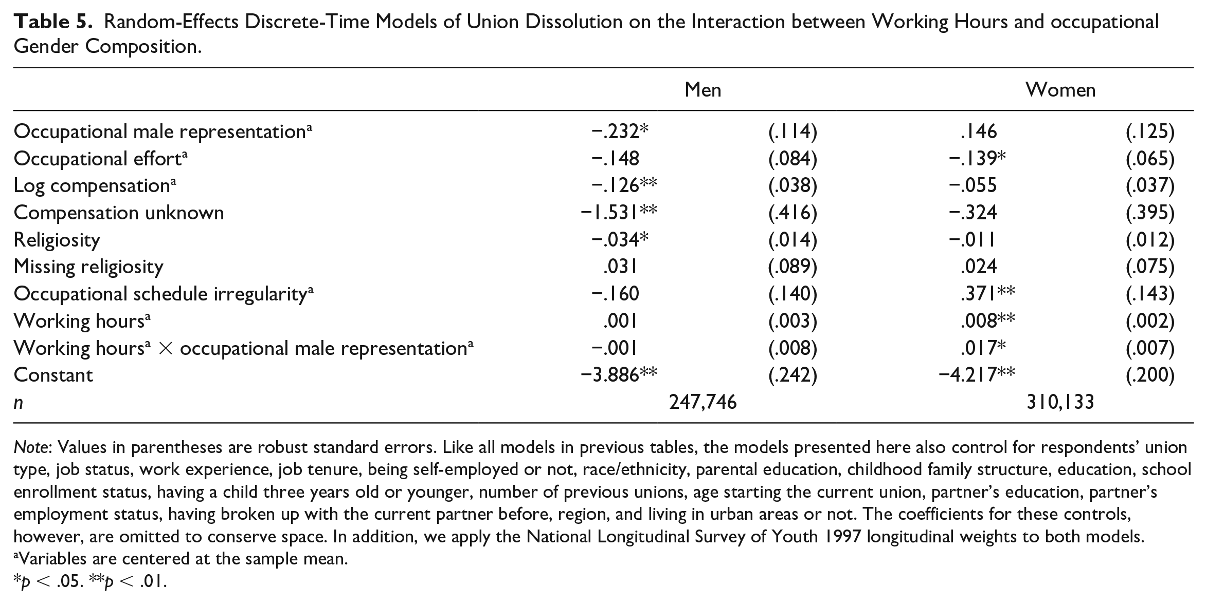
Note: Values in parentheses are robust standard errors. Like all models in previous tables, the models presented here also control for respondents’ union type, job status, work experience, job tenure, being self-employed or not, race/ethnicity, parental education, childhood family structure, education, school enrollment status, having a child three years old or younger, number of previous unions, age starting the current union, partner’s education, partner’s employment status, having broken up with the current partner before, region, and living in urban areas or not. The coefficients for these controls, however, are omitted to conserve space. In addition, we apply the National Longitudinal Survey of Youth 1997 longitudinal weights to both models.

Variables are centered at the sample mean.

p < .05. **p < .01.

Results from Table 5 are consistent with hypothesis 2; women who spend more time in male-typed occupations are especially likely to experience union instability. To illustrate the results, compared to women in occupations with an relatively balanced gender ratio (i.e., the sample mean, male representation = .48), those in a male-typed occupation—say, one in which 80 percent of the workers are male—experience a 6 percent increase in the odds of exiting a union in a given month when working 10 hours above the mean number of hours (exp[.017 × 0.32 × 10] = 1.06). Working hours, however, does not modify the association between working in gender-atypical occupations and union instability for men.

The asymmetrical results for men and women regarding the interaction between working hours and occupational gender ratio suggest that an exposure-based interpretation of the significant interaction effect for women is unlikely valid. If enhanced opportunities to meet new partners, instead of heightened job strain, explain why spending more time in gender-atypical occupations accelerates women’s union dissolution, we should find similar results for men. We do not, however. Thus, the gender asymmetry in Table 5 is more congruent with the argument that men in female-typed occupations tend not to encounter hostile coworkers or suspicion of their competency the way women in male-typed occupations do.

Conclusions

Social scientists have long been interested in how working in male- or female-typed occupations affects workers but have rarely examined how occupational gender composition is linked to workers’ family lives. In this study, we provide clear evidence that men and women working in gender-atypical occupations experience greater instability of their intimate unions, compared with their counterparts in gender-balanced or gender-typical occupations. We argue that the psychological strain derived from working in gender-atypical occupations is likely to affect individuals’ interactions with their intimate partners, thus increasing their union instability. At the same time, we consider several other mechanisms that could explain the association between working in gender-atypical occupations and union instability. We find no support that required work effort, opportunities to meet members of the other sex, values about family, or work schedules of female-type occupations explain the greater union instability for men in such occupations. The lower compensation of female-dominant occupations, compared with gender-balanced or male-typed occupations, mediates a moderate amount of the association between working in a gender-atypical occupation and union instability for men, but a considerable amount of this association remains after we account for compensation. Because our analysis rules out many alternative pathways, we suggest that the remaining association between working in female-typed occupations and union instability for men reflects the role strain that men in such occupations are likely to experience.

For women, we similarly find little support that required work effort, exposure to members of the other sex, or values about family account for the link between occupational gender composition and union instability. There is also no evidence that the greater compensation of male-typed occupations explains the higher union dissolution hazard among women in such occupations. Irregular, unpredictable schedules, however, mediate nearly half the effect of occupational male representation on the hazard of union dissolution. That is to say, a main reason that women in male-typed occupations experience greater union instability is that such occupations tend to have less regular schedules. In contrast to schedule irregularity, long working hours per se explain little of why women in gender-atypical occupations experience greater union instability. Our analysis nevertheless shows that working long hours in male-dominant occupations is especially conducive to union dissolution for women. Because this finding is consistent with the argument that the hostility and stress women face in male-typed occupations increase with the amount of time they spend at work, and because our extensive list of alternative mechanisms cannot account for the entire effect of occupational gender composition on union dissolution, we suggest that the job strain associated with working in gender-atypical occupations partially explains the greater union instability that women in these occupations experience.

Aside from the link between occupational gender composition and union stability, two findings from our study are notable. First, we show that people working in occupations that require greater effort actually have more stable unions, despite human capital theorists’ claim that effort put into work diminishes time and energy available for the family (Becker 1985). Even for women, working in effort-demanding occupations does not necessarily diminish their ability to maintain an intimate relationship; in fact, it seems to have positive spillover effects on private life, leading to greater union stability. This finding suggests that women may not need to trade work effort for family maintenance effort, as postulated by human capital theory.

Second, we find that having routine and predictable work schedules is an essential contributor to women’s union stability. This result echoes prior research showing that schedule control reduces work-family conflict and psychological stress (Kelly et al. 2014; Moen et al. 2016), both of which can jeopardize an intimate relationship. The fact that schedule irregularity does not affect men’s union stability suggests that the stress and conflict caused by this irregularity harm men’s relationship quality less, perhaps because men are more likely to be excused even when their work schedules interfere with family lives.

Although our analysis suggests that the job or role strain associated with working in gender-atypical occupations is likely to explain the lower union stability for men and women in such occupations, we must acknowledge the limitation of lacking a direct measure of such strain. We nevertheless note that ethnographic research has frequently documented the psychological strain that men and women in gender-atypical occupations experience. Moreover, we show that women’s union instability increase when they spend more hours working in gender-atypical occupations, whereas men do not. This pattern is consistent with claims found in prior research that men and women face somewhat different sources of strain when they work in gender-atypical occupations. The fact that we can exclude many other potential pathways further makes it likely that job or role strain partly accounts for the greater union instability of individuals in gender-atypical occupations. Of course, we cannot completely rule out the existence of unobserved factors that account for both individuals’ occupational choices and union instability. Our inclusion of individual-level random effects in the models, however, addresses the issue of unobserved heterogeneity to some extent (Steele et al. 2004). We also tested for the possibility that unmodeled individual characteristics simultaneously predict both gender-atypical occupation and union dissolution, and the results rejected this possibility.⁸ We therefore think that unobserved heterogeneity as an alternative argument is fairly unlikely.

At a more general level, our finding that financial compensation mediates some of the effect of working in gender-atypical occupations for men but not for women has implications for our understanding of how economic prospects shape the risk for union dissolution. Recent studies show that comparatively high income and stable employment have continued to reduce men’s risk for divorce, but they no longer increased women’s risk in recent years (Killewald 2016; Schwartz and Gonalons-Pons 2016). On the basis of the experiences of a contemporary cohort of women and men, our analysis of the roles of financial compensation provides additional evidence for this gender asymmetry. Even though occupations are still relevant to women’s union dissolution risk, the relevance generally has to do with the nonpecuniary aspects of occupations.

This study also helps advance the general knowledge of the interface between family and work. By showing that beyond employment status and earnings, specific occupational attributes are also important to the risk for union dissolution, our study suggests that the contexts, activities, and requirements of occupations have the potential to shape workers’ family dynamics. The somewhat different findings for men and women regarding which occupational characteristics are linked to union stability further suggests that the working conditions that enhance or reduce relationship quality vary somewhat by the workers’ gender roles. Future research on couple dynamics should therefore attend to the specific working conditions to which men and women are subjected.

Footnotes

Appendix

Table A1.

Descriptive Statistics of the Analytic Sample.

	Men		Women
Variable	Mean	SD	Mean	SD
Duration of the union
≤12 months	.21		.20
13–24 months	.16		.15
25–48 months	.23		.22
49–84 months	.22		.22
≥85 months	.18		.21
With a job	.88		.72
Self-employed	.08		.05
Years of work experience	8.94	(4.21)	7.70	(4.26)
Years of job tenure^a	3.18	(3.09)	2.83	(2.84)
Occupational male representation^a	.68	(.26)	.31	(.21)
Occupational effort^a	3.82	(.34)	3.88	(.38)
Log compensation^a	9.77	(3.76)	7.58	(4.96)
Compensation unknown	.05		.04
Occupational recognition^a	3.22	(1.21)	3.30	(1.13)
Occupational sociability^a	4.10	(.29)	4.32	(.26)
Occupational schedule irregularity^a	1.34	(.22)	1.21	(.18)
Working hours^a	40.47	(12.35)	34.80	(13.13)
Importance of family	2.18	(.81)	2.47	(.70)
Missing family importance	.08		.11
Religiosity	2.69	(1.93)	2.84	(1.92)
Missing religiosity	.03		.04
Race/ethnicity
Non-Hispanic white	.70		.74
Black	.12		.09
Hispanic	.14		.13
Other	.04		.04
Parental education
Less than high school	.14		.13
High school	.33		.32
Some college	.24		.26
College and more	.24		.25
Parent education unknown	.05		.05
Childhood family structure
Two biological parents	.49		.47
Single mother	.32		.35
Stepfamily	.06		.07
Other types of family	.11		.09
Family structure unreported	.02		.01
Respondent’s education
Less than high school	.12		.11
High school	.35		.32
Some college	.29		.29
College and more	.21		.26
Missing education	.03		.03
Region of residence
Northeast	.14		.13
North Central	.26		.23
South	.32		.35
West	.19		.20
Region missing	.10		.09
Urban residence
Rural	.21		.23
Urban	.69		.68
Unknown	.10		.09
School enrollment
Not enrolled	.91		.87
Enrolled	.09		.13
Unknown enrollment status	.00		.00
Any child age three or younger
No	.56		.56
Yes	.42		.43
Unknown	.02		.01
Number of prior unions	1.48	(.89)	1.63	(1.03)
Union type
Marriage	.56		.60
Cohabiting union	.44		.40
Age starting current union	23.46	(3.54)	22.48	(3.65)
Ever broken up with current partner	.07		.09
Partner employment status
Not employed	.30		.11
Employed	.67		.86
Unreported	.03		.03
Partner education
Less than high school	.11		.13
High school	.29		.32
Some college	.23		.25
College and more	.29		.22
Unknown	.08		.08
Number of person-months	247,746		310,133

Note: All the values are calculated using the person-month analytic sample, with the National Longitudinal Survey of Youth 1997 longitudinal weights applied. All variables without the standard deviation presented are dummy variables, while the ones with the standard deviation are continuous variables.

The values are calculated on the basis of the person-month observations in which a job was present.

Funding

The author(s) disclosed receipt of the following financial support for the research, authorship, and/or publication of this article: This study was supported by a research grant (106-2410-H-002-169-MY2) awarded to Janet Chen-Lan Kuo by the Research Institute for the Humanities and Social Sciences, Ministry of Science and Technology, Taiwan (R.O.C). An earlier version of the article was presented at the 2019 Population Association of America Annual Meeting in Austin, Texas, where the authors received valuable comments.

ORCID iD

Wei-hsin Yu

Notes

Author Biographies

Wei-hsin Yu is a professor in the Department of Sociology at the University of California, Los Angeles, specializing in the areas of social stratification and gender inequality. Her recent work has addressed earnings and attitudinal differences between women and men, job insecurity and its consequences, and the dynamics of marriage and relationship formation. She has published two books and numerous articles in academic journals including American Sociological Review, Social Forces, and Demography.

Janet Chen-Lan Kuo is an associate professor of sociology at the National Taiwan University. Her research focuses on the intersection of work and family life and its implications for workers’ family relationships, employment outcomes, and marriage and fertility intentions and behavior.

References

Becker

Gary S.

1985. “Human Capital, Effort, and the Sexual Division of Labor.” Journal of Labor Economics 3(1):33–58.

Becker

Gary S.

1991. A Treatise on the Family. Cambridge, MA: Harvard University Press.

Bielby

Denise D.

Bielby

William T.

1988. “She Works Hard for the Money: Household Responsibilities and the Allocation of Work Effort.” American Journal of Sociology 93(5):1031–59.

Blossfeld

Hans-Peter

Müller

Rolf

. 2002. “Union Disruption in Comparative Perspective: The Role of Assortative Partner Choice and Careers of Couples.” International Journal of Sociology 32(4):3–35.

Breen

Richard

Karlson

Kristian Bernt

Holm

Anders

. 2013. “Total, Direct, and Indirect Effects in Logit and Probit Models.” Sociological Methods & Research 42(2):164–91.

Budig

Michelle J.

2002. “Male Advantage and the Gender Composition of Jobs: Who Rides the Glass Escalator?” Social Problems 49(2):258–77.

Cech

Erin

Rubineau

Brian

Silbey

Susan

Seron

Caroll

. 2011. “Professional Role Confidence and Gendered Persistence in Engineering.” American Sociological Review 76(5):641–66.

Cha

Youngjoo

. 2013. “Overwork and the Persistence of Gender Segregation in Occupations.” Gender & Society 27(2):158–84.

Chamberlain

Gary

. 1988. “Heterogeneity, Omitted Variable Bias, and Duration Dependence.” Pp. 3–38 in Longitudinal Analysis of Labor Market Data, edited by J. J.

Heckman

Singer

Cambridge, UK: Cambridge University Press.

10.

Cognard-Black

Andrew J.

2004. “Will They Stay, or Will They Go? Sex-Atypical Work among Token Men Who Teach.” Sociological Quarterly 45(1):113–39.

11.

Davis

Shannon N.

Greenstein

Theodore N.

2009. “Gender Ideology: Components, Predictors, and Consequences.” Annual Review of Sociology 35:87–105.

12.

Doiron

Denise

Mendolia

Silvia

. 2012. “The Impact of Job Loss on Family Dissolution.” Journal of Population Economics 25(1):367–98.

13.

Dryburgh

Heather

. 1999. “Work Hard, Play Hard: Women and Professionalization in Engineering—Adapting to the Culture.” Gender & Society 13(5):664–82.

14.

England

Paula

. 2010. “The Gender Revolution: Uneven and Stalled.” Gender & Society 24(2):149–66.

15.

England

Paula

Farkas

George

Kilbourne

Barbara Stanek

Dou

Tomas

. 1988. “Explaining Occupational Sex Segregation and Wages: Findings from a Model with Fixed Effects.” American Sociological Review 53(4):544–58.

16.

Glass

Jennifer

. 1990. “The Impact of Occupational Segregation on Working Conditions.” Social Forces 68(3):779–96.

17.

Glass

Jennifer L.

Sassler

Sharon

Levitte

Yael

Michelmore

Katherine M.

2013. “What’s So Special about STEM? A Comparison of Women’s Retention in STEM and Professional Occupations.” Social Forces 92(2):723–56.

18.

Goldin

Claudia

. 2014. “A Grand Gender Convergence: Its Last Chapter.” American Economic Review 104(4):1091–119.

19.

Gorman

Elizabeth H.

Kmec

Julie A.

2007. “We (Have to) Try Harder: Gender and Required Work Effort in Britain and the United States.” Gender & Society 21(6):828–56.

20.

Henly

Julia R.

Lambert

Susan J.

2014. “Unpredictable Work Timing in Retail Jobs: Implications for Employee Work–Life Conflict.” ILR Review 67(3):986–1016.

21.

Henson

Kevin D.

Rogers

Jackie Krasas

. 2001. “‘Why Marcia You’ve Changed!’ Male Clerical Temporary Workers Doing Masculinity in a Feminized Occupation.” Gender & Society 15(2):218–38.

22.

Inanc

Hande

. 2018. “Unemployment, Temporary Work, and Subjective Well-Being: The Gendered Effect of Spousal Labor Market Insecurity.” American Sociological Review 83(3):536–66.

23.

Kalil

Ariel

Ziol-Guest

Kathleen M.

Epstein

Jodie Levin

. 2010. “Nonstandard Work and Marital Instability: Evidence from the National Longitudinal Survey of Youth.” Journal of Marriage and Family 72(5):1289–300.

24.

Kalmijn

Matthijs

Loeve

Anneke

Manting

Dorien

. 2007. “Income Dynamics in Couples and the Dissolution of Marriage and Cohabitation.” Demography 44(1):159–79.

25.

Kalmijn

Matthijs

Poortman

Anne-Rigt

. 2006. “His or Her Divorce? The Gendered Nature of Divorce and Its Determinants.” European Sociological Review 22(2):201–14.

26.

Kanter

Rosabeth Moss

. 1977a. Men and Women of the Corporation. New York: Basic Books.

27.

Kanter

Rosabeth Moss

. 1977b. “Some Effects of Proportions on Group Life: Skewed Sex Ratios and Responses to Token Women.” American Journal of Sociology 82(5):965–90.

28.

Kaufman

Gayle

. 2000. “Do Gender Role Attitudes Matter? Family Formation and Dissolution among Traditional and Egalitarian Men and Women.” Journal of Family Issues 21(1):128–44.

29.

Kelly

Erin L.

Moen

Phyllis

Oakes

J. Michael

Fan

Wen

Okechukwu

Cassandra

Davis

Kelly D.

Hammer

Leslie B.

, et al. 2014. “Changing Work and Work-Family Conflict: Evidence from the Work, Family, and Health Network.” American Sociological Review 79(3):485–516.

30.

Kilbourne

Barbara Stanek

Farkas

George

Beron

Kurt

Weir

Dorothea

England

Paula

. 1994. “Returns to Skill, Compensating Differentials, and Gender Bias: Effects of Occupational Characteristics on the Wages of White Women and Men.” American Journal of Sociology 100(3):689–719.

31.

Killewald

Alexandra

. 2016. “Money, Work, and Marital Stability: Assessing Change in the Gendered Determinants of Divorce.” American Sociological Review 81(4):696–719.

32.

Kmec

Julie A.

Gorman

Elizabeth H.

2010. “Gender and Discretionary Work Effort: Evidence from the United States and Britain.” Work and Occupations 37(1):3–36.

33.

Kohler

Ulrich

Karlson

Kristian Bernt

Holm

Anders

. 2011. “Comparing Coefficients of Nested Nonlinear Probability Models.” Stata Journal 11(3):420–38.

34.

Lupton

Ben

. 2006. “Explaining Men’s Entry into Female-Concentrated Occupations: Issues of Masculinity and Social Class.” Gender, Work & Organization 13(2):103–28.

35.

Lyngstad

Torkild

Jalovaara

Marika

. 2010. “A Review of the Antecedents of Union Dissolution.” Demographic Research 23(10):257–92.

36.

Mandel

Hadas

. 2013. “Up the Down Staircase: Women’s Upward Mobility and the Wage Penalty for Occupational Feminization, 1970–2007.” Social Forces 91(4):1183–207.

37.

Maume

David J.

Jr.

1999. “Occupational Segregation and the Career Mobility of White Men and Women.” Social Forces 77(4):1433–59.

38.

McClendon

David

Kuo

Janet Chen-Lan

Raley

R. Kelly

. 2014. “Opportunities to Meet: Occupational Education and Marriage Formation in Young Adulthood.” Demography 51(4):1319–44.

39.

McClintock

Elizabeth Aura

. 2017. “Occupational Sex Composition and Gendered Housework Performance: Compensation or Conventionality?” Journal of Marriage and Family 79(2):475–510.

40.

McClintock

Elizabeth Aura

. 2020. “Occupational Sex Composition and Marriage: The Romantic Cost of Gender-Atypical Jobs.” Journal of Marriage and Family 82(3):911–33.

41.

McKinnish

Terra G.

2007. “Sexually Integrated Workplaces and Divorce: Another Form of on-the-Job Search.” Journal of Human Resources 42(2):331–52.

42.

Mennino

Sue Falter

Rubin

Beth A.

Brayfield

April

. 2005. “Home-to-Job and Job-to-Home Spillover: The Impact of Company Policies and Workplace Culture.” Sociological Quarterly 46(1):107–35.

43.

Miller

Gloria E.

2004. “Frontier Masculinity in the Oil Industry: The Experience of Women Engineers.” Gender, Work & Organization 11(1):47–73.

44.

Moen

Phyllis

Kelly

Erin L.

Fan

Wen

Lee

Shi-Rong

Almeida

David

Kossek

Ellen Ernst

Buxton

Orfeu M.

2016. “Does a Flexibility/Support Organizational Initiative Improve High-Tech Employees’ Well-Being? Evidence from the Work, Family, and Health Network.” American Sociological Review 81(1):134–64.

45.

Mood

Carina

. 2010. “Logistic Regression: Why We Cannot Do What We Think We Can Do, and What We Can Do about It.” European Sociological Review 26(1):67–82.

46.

Palmer

Helen T.

Lee

Jo Ann

. 1990. “Female Workers’ Acceptance in Traditionally Male-Dominated Blue-Collar Jobs.” Sex Roles 22(9):607–26.

47.

Pearce

Lisa D.

Thornton

Arland

. 2007. “Religious Identity and Family Ideologies in the Transition to Adulthood.” Journal of Marriage and Family 69(5):1227–43.

48.

Poortman

Anne-Rigt

. 2005. “How Work Affects Divorce: The Mediating Role of Financial and Time Pressures.” Journal of Family Issues 26(2):168–95.

49.

Presser

Harriet B.

2000. “Nonstandard Work Schedules and Marital Instability.” Journal of Marriage and Family 62(1):93–110.

50.

Qian

Yue

Fan

Wen

. 2019. “Men and Women at Work: Occupational Gender Composition and Affective Well-Being in the United States.” Journal of Happiness Studies 20:2077–99.

51.

Roxburgh

Susan

. 1996. “Gender Differences in Work and Well-Being: Effects of Exposure and Vulnerability.” Journal of Health and Social Behavior 37(3):265–77.

52.

Sayer

Liana C.

2005. “Gender, Time and Inequality: Trends in Women’s and Men’s Paid Work, Unpaid Work and Free Time.” Social Forces 84(1):285–303.

53.

Sayer

Liana C.

Bianchi

Suzanne M.

2000. “Women’s Economic Independence and the Probability of Divorce: A Review and Reexamination.” Journal of Family Issues 21(7):906–43.

54.

Schneider

Daniel

. 2012. “Gender Deviance and Household Work: The Role of Occupation.” American Journal of Sociology 117(4):1029–72.

55.

Schwartz

Christine R.

Gonalons-Pons

Pilar

. 2016. “Trends in Relative Earnings and Marital Dissolution: Are Wives Who Outearn Their Husbands Still More Likely to Divorce?” Russell Sage Foundation Journal of the Social Sciences 2(4):218–36.

56.

Simpson

Ruth

. 2004. “Masculinity at Work: The Experiences of Men in Female Dominated Occupations.” Work, Employment and Society 18(2):349–68.

57.

Simpson

Ruth

. 2005. “Men in Non-traditional Occupations: Career Entry, Career Orientation and Experience of Role Strain.” Gender, Work & Organization 12(4):363–80.

58.

Snyder

Karrie Ann

Green

Adam Isaiah

. 2008. “Revisiting the Glass Escalator: The Case of Gender Segregation in a Female Dominated Occupation.” Social Problems 55(2):271–99.

59.

South

Scott J.

Trent

Katherine

Shen

Yang

. 2001. “Changing Partners: Toward a Macrostructural-Opportunity Theory of Marital Dissolution.” Journal of Marriage and Family 63(3):743–54.

60.

Steele

Fiona

Goldstein

Harvey

Browne

William

. 2004. “A General Multilevel Multistate Competing Risks Model for Event History Data, with an Application to a Study of Contraceptive Use Dynamics.” Statistical Modelling 4(2):145–59.

61.

Stier

Haya

Yaish

Meir

. 2014. “Occupational Segregation and Gender Inequality in Job Quality: A Multi-level Approach.” Work, Employment and Society 28(2):225–46.

62.

Taylor

Catherine J.

2010. “Occupational Sex Composition and the Gendered Availability of Workplace Support.” Gender & Society 24(2):189–212.

63.

Thornton

Arland

Axinn

William G.

Teachman

Jay D.

1995. “The Influence of School Enrollment and Accumulation on Cohabitation and Marriage in Early Adulthood.” American Sociological Review 60(5):762–74.

64.

Usui

Emiko

. 2008. “Job Satisfaction and the Gender Composition of Jobs.” Economics Letters 99(1):23–26.

65.

Watts

Jacqueline H.

2007. “Porn, Pride and Pessimism: Experiences of Women Working in Professional Construction Roles.” Work, Employment and Society 21(2):299–316.

66.

Weeden

Kim A.

Newhart

Mary

Gelbgiser

Dafna

. 2018. “Occupational Segregation.” Pathways (Special Issue: State of the Union 2018):30–33.

67.

Wharton

Amy S.

Blair-Loy

Mary

. 2006. “Long Work Hours and Family Life: A Cross-National Study of Employees’ Concerns.” Journal of Family Issues 27(3):415–36.

68.

Williams

Christine L.

1992. “The Glass Escalator: Hidden Advantages for Men in the “Female” Professions.” Social Problems 39(3):253–67.

69.

Williams

Christine L.

1995. Still a Man’s World: Men Who Do Women’s Work. Berkeley: University of California Press.

70.

Lawrence L.

2003. “Event History Models for Life Course Analysis.” Pp. 477–502 in Handbook of the Life Course, edited by J. T.

Mortimer

Shanahan

M. J.

New York: Kluwer Academic/Plenum.

71.

Yamaguchi

Kazuo

. 1991. Event History Analysis. Newbury Park, CA: Sage.

Gender-Atypical Occupations and Instability of Intimate Unions: Examining the Relationship and Mechanisms

Abstract

Keywords

Gender-Atypical Occupations, Job Strain, and Union Dissolution

Alternative Pathways

Required Work Effort

Economic Prospects

Exposure

Family Values

Work Schedules

Data

Variables and Measurement

Analytic Strategy

Results

Conclusions

Footnotes

Appendix

Funding

ORCID iD

Notes

Author Biographies

References