
Abstract
This paper investigated the role of resource levels and efficiency of resource use in the underperformance of schools designated as Comprehensive Support and Improvement (CSI) schools under the Every Student Succeeds Act. Using a novel cost-modeling approach, we estimated the amount of spending needed by schools to make meaningful improvement and compared this with actual spending to gauge underfunding. We estimated efficiency by comparing actual outcomes with expected outcomes, considering resource levels, demographics, and other characteristics. Our findings revealed that CSI schools, which disproportionately serve high-need students, are both underfunded and inefficient. Improving efficiency could address nearly a third of the performance gap between CSI schools and the statewide average. However, underfunding was the larger contributor to underperformance, with the additional funding needs of CSI schools vastly exceeding the additional ~$400 per student these schools currently receive in school-improvement funding.
Keywords
Introduction
Broadly speaking, from a theory of economic production, there are two drivers in the production of output—inputs and efficiency. As described by Hanushek (1986), “the standard conceptual framework indicates that, if two production processes are using the same inputs, any systematic difference in outputs reflects technical inefficiency” (p. 1166). Applying this concept to education, where production of outputs is interpreted as student outcomes, there are two broad ways in which student outcomes can be improved: (a) more efficient use of resources, such as funding, teachers, or time, and (b) increasing the quantity and/or quality of resources.
The accountability theory of action works from a similar premise—that education outcomes can be improved through a combination of (a) increased efficiency of resource use and (b) additional resources. Educational accountability begins with the measurement of performance and differentiating performance levels across educational units. The educational units that are the primary focus of federal accountability and of this study are schools. Accountability is then intended to induce improvements to student performance, particularly in the lowest-performing schools deemed most in need of improvement by increasing the efficiency of resource use and providing additional resources and supports. As stated by Ladd (1996) in describing accountability, “one can take the perspective of managerial efficiency, which starts with existing resources and asks how accountability . . . can be designed to maximize learning. Alternatively, one can start with some specific outcome goals and ask how many more resources would be needed in some districts or schools relative to others to achieve those goals” (p. 5).
Over the past three decades, the Elementary and Secondary Education Act, the landmark federal legislation aimed at providing more equal access to education for all students and especially those who are economically disadvantaged, has included accountability requirements. The accountability theory of action posits that the public reporting of school results, as well as the establishment of consequences for low performance, will increase motivation and effort among educators and will provide information that allows education leaders to allocate resources to where they are most needed, including to low-performing schools (Fuhrman, 2004; O’Day, 2004). Despite evidence that federal accountability policy has moved the needle on student outcomes (e.g., Dee & Jacob, 2011), accountability policy has not led to the widespread improvement that its advocates had hoped for (Spurrier et al., 2020).
One possible reason that accountability policies have not lived up to expectations is their overreliance on improvement through increased efficiency and a failure to provide sufficient resources to implement the strategies and interventions necessary to improve low-performing schools. The limited improvement among persistently low-performing schools and the growing gap in performance between low- and high-performing students (National Assessment of Educational Progress, 2022) suggests that intervention in low-performing schools has not been successful and that broader access to high-quality educational opportunities is needed.
The language of the Every Student Succeeds Act of 2015 (ESSA), the most recent reauthorization of the Elementary and Secondary Education Act, placed more emphasis on providing schools with supports and addressing resource inequities compared with its predecessor, the No Child Left Behind Act of 2002 (NCLB). As such, there was an effort to reframe accountability as something other than punitive and to deemphasize the consequences (Le Floch et al., 2024a). ESSA required that states designate the lowest-performing 5% of schools for comprehensive support and improvement (CSI) and schools with low-performing groups of students for targeted support and improvement (TSI) or additional targeted support and improvement (ATSI). CSI schools must develop improvement plans guided by a needs assessment, but there are few requirements for how to intervene in these schools other than requiring at least one evidence-based intervention. Even less is required by the law of TSI/ATSI schools. By design, ESSA focused school-improvement efforts on a smaller set of the lowest-performing schools compared with NCLB (Le Floch et al., 2024b), with the intent that state and local education agencies would be able to concentrate limited capacity and resources on relatively few very high-need schools.
ESSA included several other features signaling the intent to provide additional resources to schools receiving accountability designations. Most directly, the law required that at least 7% of Title I, Part A funding be set aside to support school improvement in schools designated under the federal accountability system. ESSA also included provisions that require examining resource allocation within districts, including that states conduct resource-allocation reviews within districts with significant numbers of schools designated as CSI or TSI/ATSI under federal accountability and that districts with CSI schools identify and address resource inequities within their districts. Despite these requirements, there was little guidance for how these reviews of resource allocation should occur and how to act on identified inequities. In short, the mechanisms for providing additional fiscal resources to schools with accountability designations under ESSA were relatively weak, making it uncertain whether such schools would receive increased funding in amounts that would support meaningful improvement.
Given the emphasis of accountability policy on both efficiency and providing additional resources and supports, we conducted a series of analyses examining the resources provided to schools receiving accountability designations under ESSA (with an emphasis on CSI schools) and the level of efficiency of those schools. The following research questions (RQs) define our objectives and guide our analyses:
For RQ1, we conducted descriptive analyses that provided contextual information regarding the characteristics of schools with accountability designations and the extent of the challenges they faced with respect to student need and outcomes. To address RQ2, we conducted descriptive analyses and used a school fixed-effects model to examine whether CSI schools received additional resources under existing policy. We used cost-function modeling, an approach most often applied in state adequacy studies, to address RQ3 regarding the spending levels and additional funding that would be required for CSI and TSI/ATSI schools to make meaningful improvement. Lastly, for RQ4, we extended the results of the cost-function model to calculate a measure of efficiency for each school, which we defined as the difference between actual and expected outcomes and where expected outcomes were predicted based on a regression model that included a measure of funding as well as school demographics and other school characteristics. As such, our calculation of efficiency was a relative measure of technical efficiency, where higher values represented higher outcomes after controlling for differences in funding levels, school demographics, and other school characteristics (Schwartz & Stiefel, 2001). We then used descriptive analyses to examine the levels of efficiency in CSI and TSI/ATSI schools compared with nondesignated schools. Furthermore, we decomposed the low performance of schools receiving accountability designations into the portion of performance outcomes attributable to underfunding and inefficiency.
Our study used Ohio as a case study state. Ohio is a compelling case study because it is diverse racially, socioeconomically, and geographically, with high-need districts and schools in both urban and more rural areas. In addition, Ohio’s current level of spending on education is on par with the national average (U.S. Department of Education, 2023), and Ohio uses an index-based approach to measure school performance and assign accountability designations to schools, similar to most states. Additional details regarding Ohio’s system of identifying and supporting designated schools can be found in Sections A.1 and A.2 of Appendix A in the online version of the journal.
Our results indicated that CSI schools faced substantial challenges in student performance and served disproportionately high-need student populations. Despite the magnitude of their challenges and needs, the additional funding and spending they received was quite meager—around $400 per pupil. The results of our cost-function model suggested that CSI schools would need an additional $10,000 per student, on average, to reach the statewide average outcome or an additional $5,500 to meet a lower meaningful outcome target. The magnitude of the gap in funding indicates that, currently, there is a misalignment between the level of need in CSI schools and their ability to address those needs with their existing level of resources. CSI schools are also relatively inefficient compared with nondesignated schools, suggesting that there is also room for improvement in how these schools use the resources they have. However, if these schools improved their level of efficiency to the statewide average, they still would be vastly underperforming non-designated schools. As such, both broad drivers of performance (i.e., efficiency and inputs) should be addressed in CSI schools, but attempting to address efficiency without addressing the underfunding of these schools likely will result in limited and insufficient gains. We also show that CSI schools vary in the extent to which inefficiency and underfunding contribute to their low performance. Knowing the severity of those two issues for each school could help technical assistance providers in states and districts tailor the types of supports and interventions for CSI schools.
Policy Context/Literature Review
Education Spending, Student Outcomes, and Efficiency
Over the last decade, methods focused on causal inference have shown that increases in spending have positive effects on student outcomes, particularly so for students in poverty. Several studies used the timing of state court decisions and school finance reforms to show that the increased spending from these reforms improved student outcomes overall and improved equity in outcomes (Candelaria & Shores, 2019; Jackson et al., 2016; Lafortune et al., 2018). Other studies of state-specific school finance reforms also found similar results. Roy (2011) and Hyman (2017), for example, found that increased spending in Michigan resulting from a 1994 policy change improved student assessment scores in the previously lowest-spending districts and increased postsecondary attainment. Likewise, Johnson and Tanner (2018) found that California’s change to its school funding formula led to increased high school achievement and graduation in high-poverty districts, concluding that “money targeted to students’ needs can make a significant difference in student outcomes and can narrow achievement gaps” (p. i).
Another set of recent research used the passage of close bond elections to assess the effects of increased spending as a result of passage of bond initiatives (Biasi et al., 2024; Rauscher et al., 2024). Biasi et al. (2024) found that investments in school facilities improved test scores, particularly in districts with higher rates of economic disadvantage. Rauscher et al. (2024) found that operational spending had larger effects on achievement than capital spending but that both types of spending had higher effects on achievement in low-spending districts compared with districts that already had high spending. They also found that investments in teacher salaries were among the more effective uses of increased funds for Black and low-income students.
The results of rigorous studies of the impact of additional spending on educational outcomes have been synthesized in two relatively recent meta-analyses. Jackson and Mackevicius (2024) translated findings from across the studies included in their meta-analysis into the effect of a $1,000 per pupil spending increase sustained over 4 years, finding that this amount resulted in improved test scores of 0.032 standard deviations (SDs) and college attendance by 2.8 percentage points and finding larger effects for economically disadvantaged populations. Handel and Hanushek (2023) also summarized the findings of studies examining the effects of increased spending using rigorous causal inference designs. They found that of the 16 studies that met their inclusion criteria and focused on achievement outcomes in the United States, 14 were positive and nine were statistically significant, noting that the median effect size of a 10% increase in spending was 0.07 SDs. Of the 18 studies that met their criteria and focused on attainment (i.e., graduation, dropout, and college going), all were positive, and 14 were statistically significant, and they noted that the median effect of a 10% increase in spending was a 5.7% increase in educational attainment.
Despite the relatively conclusive findings that additional spending on education tends to have a positive impact, a debate remains as to whether spending more on education is wise when there remains uncertainty about how to best use funds. As McGee (2023) wrote: “Money matters in education, but it is also clear that how money is spent, on whom, and under what circumstances have a large impact on results” (p. 3). Handel and Hanushek (2023) discussed the variation in the study results and contexts, concluding in the end that “little progress has been made in leveraging the results to uncover when more spending will have significant impacts and when it will not” (p. 216). Hanushek (2020), drawing on research showing variation in the relationships between spending and outcomes, stated: “The general conclusion from the existing work is that how resources are used is generally more important than how much is used” (p. 168). Jackson and Persico (2023) described this as a false dichotomy, noting that it is possible for schools to access more resources and use them well.
Accountability, Efficiency, and School Resources
Accountability theory of action
Figlio and Loeb (2011) broadly defined school accountability as the process of evaluating school performance on the basis of student performance measures. Our study was contextualized within the policy environment of ESSA, where states are required to designate schools with CSI and TSI/ATSI performance ratings based on a set of defined performance measures. Designated schools must (a) develop school-improvement plans guided by needs assessments with the support of their districts and (b) implement evidence-based interventions. In addition, designated schools are eligible to receive additional federal funding, and districts with CSI schools are supposed to identify and address resource inequities. The end result of this is that school performance, as measured by student performance measures, should improve in designated schools. Although the details of the accountability theory of action may have changed over the course of subsequent iterations of federal policy, the broad elements guiding state and federal accountability systems have remained consistent for several decades: measuring performance and assigning ratings based on a set of defined performance standards (O’Day & Smith, 1993), using pressure and consequences as a sources of motivation (Fuhrman, 2004), and directing supports and resources to where they are most needed (O’Day, 2004).
Most important to our study, accountability policy in education is firmly rooted in the premise that the production of educational outcomes should be more efficient, but there is also broad agreement that improving school performance requires additional resources. Related to use of accountability to improve efficiency, Fuhrman (2004) described how increased focus on performance and student outputs is traced to the influence of business leaders and economic concepts used in turning around struggling businesses, such as setting explicit goals and providing increased flexibility to workers in meeting those goals. In other words, the notion of accountability that proliferated in the 1990s and early 2000s focused less on compliance with rules and more on successfully increasing student learning and outcomes (Elmore et al., 1996). O’Day (2004) also expressed the role of accountability in monitoring the efficiency of public spending. After noting the large sum of money spent on public education, she stated: “It is reasonable for the public and its representatives to want to know where the money is going and what it is producing” (p. 15).
The accountability theory of action, as posited by Fuhrman (2004), indicates that focusing the accountability system on student performance, including public reporting of results and consequences, will make performance “the most important concern of school personnel,” resulting in devoting “energy and resources, in a concerted fashion, toward improving student performance” (p. 8). O’Day (2004) also explained that accountability is meant to draw educator attention to information that is relevant to teaching and motivate educators to increase their efforts to improve or change strategies in response to the information. In short, accountability should increase efficiency through motivation, effort, and better information.
There is also broad consensus of the importance of resources in the successful facilitation of school improvement through accountability. O’Day (2004) posited that one of the responses of successful accountability systems must be to allocate resources to where they are most needed, such as allocating resources to low-performing schools. Elmore et al. (1996) indicated that one barrier to successful implementation is resource constraints and that money is required for the “task of turning around the lowest performers” (p. 87). Peyser and Costrell (2004) noted that there are costs in accountability systems associated with supporting turnaround efforts in low-performing schools and districts and costs more broadly in providing all students with the educational opportunities necessary to attain the goals or performance targets set by state standards and accountability systems. Accountability policies and the associated requirements (e.g., testing and reporting of data, monitoring of progress, etc.) also increase administrative expenses (Neely, 2015), potentially redirecting efforts away from teaching and learning and toward compliance. Lee and Wong (2004) asserted that without providing adequate support and ensuring equity in resources and educational opportunities, accountability simply rewards advantaged schools and punishes disadvantaged ones.
Accountability and student outcomes
Studies of early accountability systems focused on statewide gains in improvement, finding that states that adopted “consequential” accountability systems and those with stronger repercussions for schools and students had larger statewide achievement gains than states with less stringent consequences or those that relied only on reporting results without consequences (Carnoy & Loeb, 2002; Hanushek & Raymond, 2005). Dee and Jacob (2011) examined the impact of NCLB on statewide achievement, finding that the mandated adoption of stronger accountability systems that contained consequences for low performance led to improved math achievement outcomes in states that did not have consequential accountability systems prior to NCLB but did not influence reading.
Studies also have also focused on the effects of accountability for individual schools that have been designated as low performing. Many of these studies relied on regression discontinuity designs that compared results of schools just below and above cutoff scores used to assign schools’ performance ratings. For example, several studies of Florida’s A–F state accountability rating system found that F ratings resulted in improved student achievement outcomes following the rating (Chakrabarti, 2007; Figlio & Rouse, 2006; Rouse et al., 2007) and attributed the improvement to the stigma of receiving a low grade rather than through the threat of consequences associated with the grade (Figlio & Rouse, 2006). Winters and Cowen (2012) performed a similar study of New York City’s A–F rating system and similarly found that an F rating led to improvement in the years subsequent to the designation, also attributing the finding to shaming, suggesting the importance of public reporting of results in motivating change.
Under NCLB waivers instituted under the Obama administration, states were to identify low-performing schools as priority schools and schools with large achievement gaps or low-performing student groups as focus schools. The set of studies examining the effect of schools receiving low-performance designations under this policy regime was rather mixed. Bonilla and Dee (2017) found positive effects of low-performance designations in Kentucky, but other studies found null results in Michigan (Hemelt & Jacob, 2017) and Louisiana (Dee & Dizon-Ross, 2019) and negative results in New York (Atchison, 2020), North Carolina (Henry & Harbatkin, 2020), and Rhode Island (Dougherty & Weiner, 2017). In explaining the negative findings, Dougherty and Weiner (2017) found that schools that were forced to implement a higher number of interventions had lower performance outcomes. Henry and Harbatkin (2020) found that the policy in North Carolina led to increased teacher turnover. In other words, the pressure resulting from accountability systems could have led to negative unintended consequences in addition to (or instead of) the intended motivational effects.
The relatively small set of studies of ESSA accountability systems thus far also has portrayed mixed findings. Researchers in Michigan have reported evidence of improved student outcomes prior to the pandemic associated with the state’s approach to supporting the lowest-performing schools under ESSA (Burns et al., 2023; Cullum & Harbatkin, 2023). Atchison et al. (2025b) found that CSI designation in Ohio resulted in worse student outcomes as measured by chronic absenteeism, graduation rates, and ACT scores, while also finding that CSI schools potentially had increased teacher and principal turnover. Atchison et al. (2025a) found no effect of CSI designation in California on high school graduation and college and career readiness but did find that schools who received low performance ratings on individual outcome indicators for graduation and college and career readiness subsequently improved their outcomes specific to those indicators, potentially highlighting the importance of clear and actionable information.
Motivational effects and unintended consequences of accountability
One of the main efficiency-based mechanisms through which accountability is assumed to improve school performance is through increasing the motivation or effort of educators. As noted by Fuhrman (2003), the intent is that accountability pressure from public disclosure of results and consequences for low performance will increase motivation, energy, and effort toward improving student outcomes, resulting in improved instruction. A recent survey of principals of low-performing schools found that ~75% of these principals thought that accountability designations “create a sense of urgency for my school to take action” (Yang & Atchison, 2024, p. 30). A sense of urgency may be a precursor to increased motivation and effort underlying the accountability theory of action, but it does not necessarily lead to productive and healthy urgency.
An alternative reaction to urgency is stress and decreased morale. Finnigan and Gross (2007) indicated that accountability policy may result in an initial increase in motivation and effort but that motivation deteriorates in schools that persistently struggle. They explained that as time went on and performance expectations were not met, teachers lost the expectation that they could accomplish the goals laid out for them. In studying a school-based incentive program, Kelley et al. (2002) found that in setting school-level goals and establishing incentives, most teachers reported making efforts to improve with the aim of meeting goals. However, they also determined that the consequences of not meeting goals can induce stress and that accountability-induced stress offsets positive motivational effects.
Whether urgency leads to increased productivity through effort and motivation or leads to negative unintended consequences such as stress depends on whether educators know the actions that are necessary to promote improvement. In the context of NCLB, Cohen et al. (2007) explain that the goals of NCLB were ambitious but that practitioners did not have sufficient capacity or knowledge in how to improve instruction. This mismatch between ambitious expectations and insufficient capacity to achieve expectations set the stage for addressing urgency in superficial ways that led to the many documented unintended consequences of NCLB, such as teaching to tests, reallocating instructional time to tested subjects at the expense of nontested subjects, and focusing improvement efforts on students closest to proficiency thresholds (Chakrabarti, 2007; Dee et al., 2013; Diamond & Spillane, 2004; Koretz, 2008; Neal & Schanzenbach, 2010; Rothstein et al., 2008). As explained by Diamond and Spillane (2004), the lowest-performing schools, which disproportionately serve poor students and students of color, face the greatest mismatch between expectations and capacity. As such, these schools are most susceptible to unintended consequences.
Accountability and allocation of resources
An enabling factor in translating urgency to productivity is the capacity to implement change. According to Cohen et al. (2007), knowing how to improve is one aspect of capacity. A second aspect is fiscal capacity to purchase the necessary staff and goods to implement the interventions and strategies necessary for improvement. 1 Successful accountability systems should allocate resources to where they are most needed, including to low-performing schools to support improvement activities (O’Day, 2004).
If reallocation of resources to low-performing schools and districts occurred in response to implementation of accountability systems, we might expect to see a corresponding increase in resources in schools and districts with higher shares of student in poverty and of color (which are most often designated as low performing under accountability systems). However, Lee and Wong (2004) found no evidence of differences between strong and weak pre-NCLB accountability states in the changes in the distributions of class size and spending along racial or socioeconomic dimensions. Although Dee et al. (2013) and Atchison (2017) did find that NCLB-induced accountability pressure increased spending overall, they did not find that the increase varied systematically across districts with different poverty levels.
Failure to find evidence of targeting resources toward higher-need schools under NCLB is not incredibly surprising given the lack of explicit policy mechanisms designed to reallocate resources under the law. Under NCLB, only a limited pot of federal funding was explicitly targeted to schools designated under the accountability system (ranging from 2 to 4% of total Title I, Part A funding; McClure, 2005). Based on a survey of district and school leaders in early implementation of NCLB, Hamilton et al. (2007) found that inadequate funding was one of the most frequently identified barriers to improvement efforts. Chambers et al. (2009) found that schools designated under NCLB accountability as needing improvement received less in Title I funding per low-income student than nonidentified schools, noting that designated schools had higher poverty rates than nondesignated schools.
Under ESSA, the amount of federal funding directed to schools receiving accountability designations increased to 7% of Title I, Part A funding. However, even at this increased level, the amount of funding provided to designated schools still was small compared with their needs. Blair et al. (2025) estimated that federal school-improvement funding for CSI schools most typically ranged from $100 to $400 per pupil across states during early implementation of ESSA accountability. Additionally, they estimated that CSI schools only spent about $345 per pupil more than comparable non-CSI schools, with the bulk of additional spending accounted for with federal funds. They concluded that CSI schools were not provided with enough additional funding to support meaningful improvement.
Also inferred from the work of Blair et al. (2025) is that states and districts did not appear to target much of their own state and local funding to CSI schools. Hyslop and Zhou (2024) found that CSI schools often spent less per pupil following their identification, largely driven by declines in spending from state and local funding sources. They concluded that state and local leaders should shield schools designated under the accountability system from budget cuts and add funding mechanisms to provide those schools with additional support through state and local funding.
Estimating the Cost of Meaningful Improvement
In school finance, the term adequacy represents the amount of spending necessary for providing all students with the opportunity to meet a given outcome goal. This spending amount is referred to as the cost (Downes & Stiefel, 2014). Educational costs vary across schools and districts according to student needs and other structural and geographic contextual factors (Baker et al., 2024; Duncombe et al., 2015). This variation in cost is consistently reflected in state education funding policies that account for differences in student needs as well as other contextual differences, such as population sparsity, district or school size, and grade levels of students served (Kolbe et al., 2020). However, there is little consensus on the magnitude of the differences in cost for different student groups or contextual factors. Furthermore, differences in cost reasonably may differ depending on the definition and interpretation of adequacy and the types of student performance outcomes that are valued in different states or locations (Downes & Stiefel, 2014; Duncombe et al., 2015).
The use of education cost functions is one approach to estimating adequacy (Downes & Stiefel, 2014; Duncombe et al., 2015). The cost-function approach uses regression-based statistical modeling to estimate education cost as a function of student outcomes, resource prices, enrollment size or scale, and measures of student need. Education cost functions typically treat the relationship between outcomes and spending as endogenous due to the fact that they may be determined simultaneously. Increased spending can drive higher outcomes through the purchase of additional educational resources. However, higher outcomes also may drive increased spending, for example, by making the district more attractive, resulting in higher property values and more local revenue. To address this endogeneity, education cost functions are typically estimated using a two-stage instrumental variables model (Baker, 2011; Baker et al., 2024; Duncombe & Yinger, 2004, 2011). In addition, cost-function models must account for differences in efficiency, where efficient schools and districts are thought to be implementing best practices (Duncombe et al., 2015) and therefore obtaining higher student outcomes at a given level of spending.
A key strength of the education cost-function approach is that it uses actual historical data to measure the empirical relationships among spending, student outcomes, and other cost factors (Baker et al., 2025a; Duncombe et al., 2015). Education cost functions also typically rely on data that are inclusive of all districts and schools within a given state, meaning that the data are necessarily representative of all contexts and combinations of different factors that characterize the costs in schools or districts (Baker et al., 2025a).
Although the education cost-function approach has typically been applied to understand the levels of adequacy and cost differentials for specific student groups statewide to inform state-level funding formulas (e.g., Atchison et al., 2024b; Taylor et al., 2018; Zhao, 2020), we apply the approach in several unique ways. First, our main emphasis is on a subset of schools that have been designated by Ohio’s accountability system as being low performing and in need of improvement. As such, we are not focused on statewide adequacy but rather on the level of resources needed to generate improvement in a smaller set of designated low-performing schools. Second, we extend the cost-function model in a unique way to examine the efficiency of schools designated by the state accountability system as low performing.
Data
To facilitate the analyses, we compiled a comprehensive school-level dataset that included (a) spending per pupil, (b) student outcomes, (c) student demographics, and (d) other contextual and geographic characteristics of schools though to affect spending from the 2017–18 to 2022–23 school years. The COVID-19 pandemic occurred during the middle to later years of data used in this study. The pandemic had substantial effects on student outcomes, levels of funding, and how schools used resources. This context should be kept in mind because the data used in this study may not be reflective of past or future trends. Through the remainder of this article, we define school years based on the year in which the school year ended. For example, we use 2018 for the 2017–18 school year. Details on the data measures/variables used in the analyses addressing each RQ are presented in Section B.1 of Appendix B in the online version of the journal. There we provide a summary of the various data used in this study.
The Ohio Department of Education and Workforce (ODEW) provided detailed fiscal data between 2018 and 2023, allowing us to calculate total spending per pupil for each school as well as categorize spending into the following functions: food services, general administration, instruction, instructional staff support, operations and maintenance, pupil support, school administration, transportation, and other nonspecified support. Definitions for these function categories are provided in Table B3 in Appendix B in the online version of the journal. Most expenditures in the data are attributed to individual schools. However, some portion of expenditures represents centralized services that are not attributed to schools but are recorded as district-level expenses. To calculate school-level per pupil expenditures accounting for all district spending, we allocated the centralized district-level expenditures to schools proportionally to each school’s share of the total district enrollment. In addition to the school-level expenditure data, we compiled school-level data on the amount of school-improvement funds provided to each school associated with Section 1003, Part A of ESSA, available through U.S. Department of Education’s ED Data Express for the school years 2018–21.
We gathered publicly available school-level outcome data including 4-year graduation rates, math and English language arts (ELA) proficiency rates, and chronic absenteeism from ODEW’s Report Card database. Using these student outcome data, we constructed an outcome factor score as a single measure using confirmatory factor analysis. The resulting measure has a mean of 0 and a standard deviation of 1. For more detail on the creation of the outcome factor score and justification for using the outcome factor score, see Section B.2 of Appendix B in the online version of the journal.
We also compiled a variety of data on school enrollment and student characteristics from ODEW’s Report Card database, including counts and percentages of students by race/ethnicity, English learner status, disability status, and grade level. Because of issues related to the distribution of the state’s measure of economic disadvantage, we opted to use the Urban Institute’s Modified Model Estimates of Poverty in Schools (MEPS) as the primary measure of economic disadvantage (see Section B.3 of Appendix B in the online version of the journal for more detail on our choice to use the MEPS).
Data on school characteristics including charter status, school type, grade levels served, ZIP Code, and urbanicity were gathered from the National Center for Education Statistics (NCES) Common Core of Data. We used the NCES’s Comparable Wage Index for Teachers (CWIFT) as a measure of geographic price differences. 2 We also compiled a number of other contextual variables including the NCES Education Demographic and Geographic Estimates income-to-poverty ratio, and ZIP Code–level variables (e.g., population density, percentage of population that is age 65 years or older, percentage of population who have a bachelor’s degree, and percentage of housing units that are vacant) from the 2020 Decennial Census.
Empirical Approach
In this section we describe each of our analyses associated with the RQ those analyses address. Collectively, our analyses cover the period between 2018 and 2023. During this time, there were two points in which new accountability designations were assigned—2019 and 2023. In addition, because data following the pandemic were insufficient for schools to meet the state criteria of consecutive years of improvement to exit their designation status, all CSI schools from the 2019 cohort were retained as CSI schools in the 2023 cohort, but additional schools became CSI schools. As such, regardless of whether we focus our analyses on the 2019 or 2023 cohort of CSI schools, the schools are largely the same set of schools. For retrospective analyses examining change over time, we focused on the schools identified in 2019, and for analyses estimating funding needed for meaningful improvement and inefficiency, we focused on the 2023 cohort because it is more contemporary.
Research Question 1
To address the first RQ, we conducted descriptive comparisons of student demographics and outcomes between Ohio public schools with different accountability designations (e.g., CSI, TSI/ATSI, and nondesignated schools) in the first year of ESSA accountability implementation (2019). To do so, we examined the percentage of student enrollment in six demographic groups (i.e., students experiencing poverty, English learners, students with disabilities, White students, Black students, and Hispanic students) and five different outcome measures (i.e., math test proficiency, ELA test proficiency, chronic absenteeism, 4-year graduation rate, and outcome factor score). For this analysis, we calculated the student-weighted average demographics or outcomes in CSI and TSI/ATSI schools, and we represented the averages for those schools as a student-weighted percentile based on the distribution of student demographics in nondesignated schools. The results can be interpreted as the percentage of nondesignated school enrollment that attended schools with demographic percentages or outcomes less than the CSI or TSI/ATSI average.
Research Question 2
To examine whether CSI or TSI/ATSI schools received additional fiscal resources, we first conducted descriptive analysis of Section 1003(a) funds. In doing so, we calculated the percentages of CSI and TSI/ATSI schools that received funding within any year between 2019 and 2021. Second, we calculated the average amount that each designation category received each year.
Next, we used a school fixed-effects regression model to compare trends in CSI school spending per pupil relative to nondesignated school spending between 2018 and 2023. 3 In addition to examining overall spending, we disaggregated spending into nine function categories (e.g., instruction, school administration, etc.). The regression model is as follows:
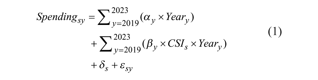
where
We treated the results of the school-fixed effects model as descriptive rather than causal. In particular, we had only 1 year of pretreatment data and therefore were unable to examine the data for the presence of parallel pretreatment trends between schools that were later designated as CSI and those that were not. Another key assumption underlying difference-in-differences analyses or event-study designs was that there were no other events that occurred concurrently with the introduction of treatment that could have differentially affected the groups of schools being compared. In this case, we were considering 2019 to be the beginning of treatment. The COVID-19 pandemic occurred shortly thereafter, along with additional federal funding allocations intended to help districts address pandemic-related challenges. As such, it seemed quite likely that other contemporaneous events occurred that could have affected CSI schools differently from non-CSI schools, limiting the extent to which we could treat the estimates as causally related to the CSI designation. Nonetheless, we felt that the analyses served a purpose in describing the relative increase in spending in CSI schools compared with non-CSI schools over this time period and provided a point of comparison with the additional amounts of funding CSI schools needed, as estimated as part of RQ3. 4
Research Question 3
To examine the additional funding needed to support meaningful gains in student performance in schools receiving accountability designations, we used cost-function modeling of a form that was documented the in peer-reviewed literature (Duncombe, 2002; Duncombe et al., 2003; Duncombe & Yinger, 1999, 2004, 2011; Kolbe et al., 2021). In particular, we used a cost-function model of the following form:

where
After the model was estimated, we used the model parameters to identify the predicted amount of spending per pupil needed for each school to achieve a target outcome level. To generate these predictions, we set the Outcomes variable to a constant value for all schools representing the target outcome level, and we set the variables representing Inefficiency to the statewide averages in the most recent year of the data (Baker, 2025). The remaining variables representing student needs, input prices, school structure, scale, and sparsity remained at the observed values for each school, allowing the predicted spending levels for each school to reflect the differences in those characteristics based on the estimated parameters for those factors describing their relationship with spending.
We generated spending predictions at two different outcome levels: (a) the statewide average and (b) a lower target, which we set at 0.5 SDs below the state average. The lower performance level was approximately the 25th percentile of performance across all schools in the state. However, 92% of students in CSI schools and 48% of students in TSI schools (based on 2023 designations) attended schools that performed below this level. By contrast, only 18% of students in nondesignated schools attended schools performing below this level. Therefore, the lower performance target represents improvement for most CSI schools and about half of TSI/ATSI schools but is at a level that nondesignated schools largely outperform.
Using the predicted spending level at each target level, we calculated the gaps in spending between actual and predicted spending to define the degree to which schools were underfunded with respect to the target outcomes. In our calculations, negative values of the gap represented underfunding with respect to meeting the target outcome level and positive values represented overfunding. We then conducted descriptive analyses examining the funding gap of schools, disaggregating the results according to accountability designations.
In Section B.4 of Appendix B in the online version of the journal, we provide additional details on the cost-function model, including the treatment of outcomes as endogenous and the selection of instruments, the selection and justification of the inefficiency measures, a presentation of the cost-function results, and validity checks.
Research Question 4
Two schools with the same characteristics and funding levels should have the same level of expected outcomes but may achieve different actual outcomes. In this example, we attribute the differences in actual outcomes to differences in efficiency of resource use. Therefore, in simple terms, we define efficiency as the difference between actual and expected outcomes. We used the following regression model, which includes the funding gap estimated based on the cost-function model, to define each school’s expected level of outcomes:

where
Efficiency, defined as the difference between actual and expected outcomes, also can be thought of as the change in school performance if the school performed at average efficiency. After accounting for change in outcomes up to the level of average efficiency, we assumed that additional needed improvement in outcomes would have to be addressed through providing additional resources. This can be explained most clearly with an example. Suppose that a school’s aggregate outcome score is −1 and that the school’s predicted outcome is −0.25. The difference between actual and expected outcomes is −0.75, meaning that the school is relatively inefficient. If the school improved in efficiency to the average, its outcome score would improve from −1 to −0.25. To reach the target of the statewide average, additional funding would be needed, but only to cover the portion of underperformance represented by the difference between the predicted outcome and the outcome target (i.e., to get from −0.25 to 0).
After calculating the efficiency measure for each school, we conducted descriptive analyses to examine the extent to which efficiency differs across schools based on accountability designation. In addition, we used the assumptions about the portion of performance that would reasonably be influenced through efficiency versus through additional resources laid out in the preceding example to decompose the underperformance of designated schools into the portion due to inefficiency versus the portion due to underfunding. Specifically, we used each school’s expected outcome as the delineation between underperformance resulting from inefficiency versus underperformance resulting from underfunding, with the portion between the target and the expected outcomes due to underfunding and any underperformance beyond the expected outcomes due to inefficiency. As a sensitivity check, we examined the robustness of our findings to the exclusion of alternative schools, which are disproportionately identified as CSI schools. These results of this robustness check are provided in Section E.1 of Appendix E in the online version of the journal.
Our approach to estimating efficiency relied on the interpretation of the difference between actual and expected outcomes (as predicted by our regression model) as the degree of efficiency. We acknowledge that there are limitations to this approach. There could be reasons other than relative efficiency for why observed and expected outcomes differ related to model specification. First, we were using a limited set of outcome measures. To the extent that schools spend their funding in ways meant to address outcomes beyond those included in our model, we may characterize schools as being less efficient than they are. Second, we may be omitting covariates that explain differences in outcomes and/or spending across schools. For example, the school demographic measures we included are poverty rate and students with disabilities and English learner percentages. Student need is likely more nuanced than the information provided by these three variables. Third, we assumed that our model had an appropriate functional form, which may not be the case. These limitations also apply to the estimation of cost using cost-function modeling. If there were important outcomes or dimensions of need we were not accounting for, we were likely underestimating cost in high-need schools.
Importantly, the limitations or potential bias in our estimates point in the direction of possibly underestimating differences in cost and overestimating differences in efficiency across schools. Outcomes, as we have characterized them from a production standpoint, are attributable to only two factors—level of resources and efficiency of resource use. Any improvements to the estimation of cost and modeling of efficiency necessarily would reduce the residual error term in the efficiency regression model (Equation 3), which we interpret as relative efficiency. This would result in attributing a greater portion of low-performing schools’ underperformance to underfunding and a smaller portion to inefficiency. As such, it is reasonable to think of our estimates of costs in low-performing/high-need schools as lower bounds and the estimates of inefficiency of these schools as upper bounds.
Results
Characteristics of ESSA Designated Schools
Students in CSI and TSI/ATSI schools were more often students of color, had disabilities, were English learners, were from low-income families, and also tended to have much lower outcomes than students in nondesignated schools. Figure 1 shows where the CSI and TSI/ATSI schools attended by the typical student ranked as a percentile among nondesignated schools, with the upper panel showing student demographics and the bottom panel showing student outcomes. For example, the CSI school attended by the typical student had a poverty rate at the 95th percentile of nondesignated schools. The figure also shows that CSI schools (and TSI/ATSI schools to a slightly lesser extent) had disproportionately high students with disabilities, English learners, and students of color and disproportionately low percentages of White students.
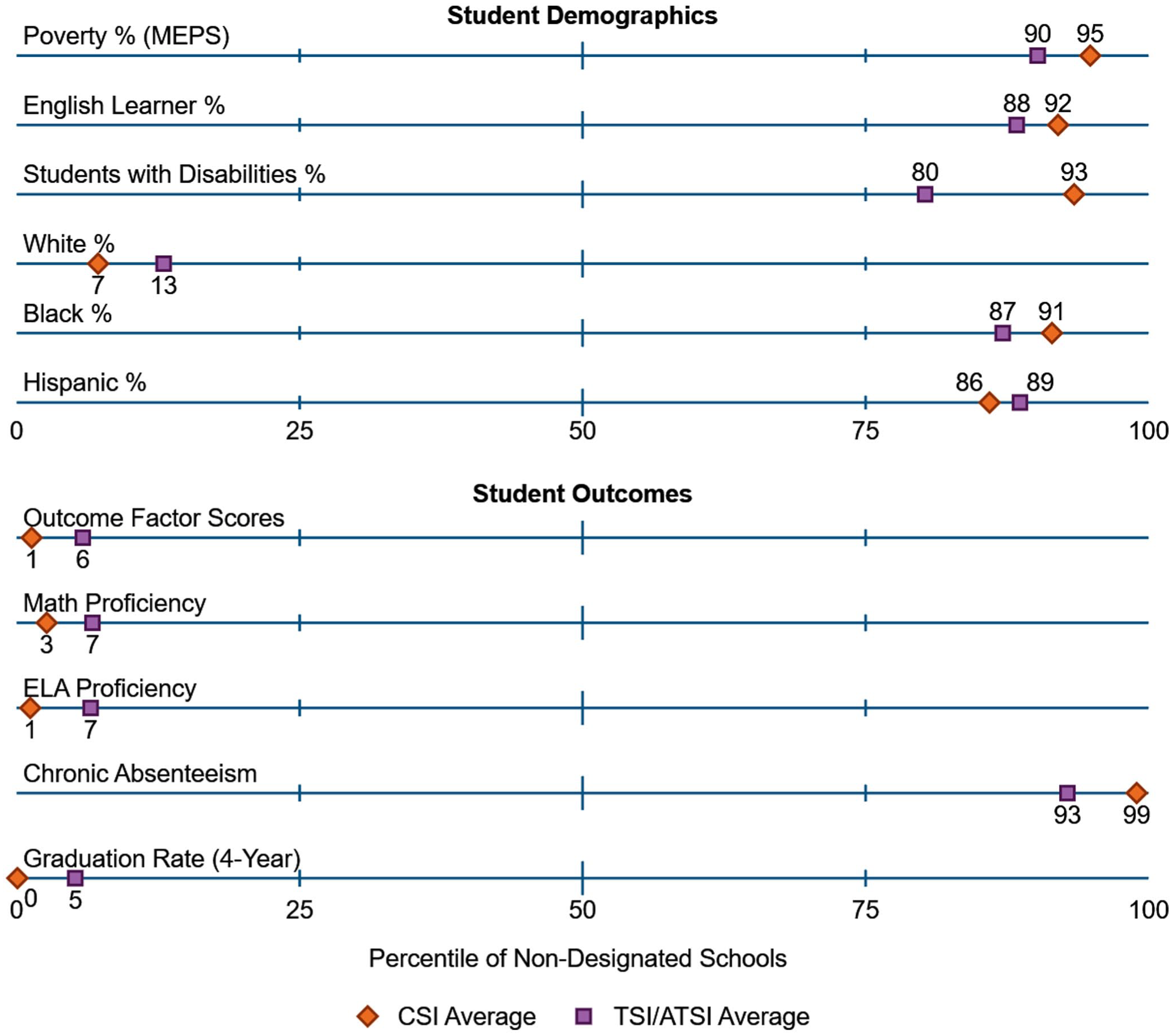
Percentile of average characteristics of CSI and TSI/ATSI schools based on the distribution of nondesignated schools (2019).
The student outcomes of CSI and TSI/ATSI schools differed from those of nondesignated schools to an even greater extent than demographics. The average of CSI schools performed at only the 1st percentile of nondesignated schools on the outcome factor score measure. In other words, 99% of students in nondesignated schools attended schools with higher performance than the CSI school pupil-weighted average. CSI schools exhibited similar levels of relative performance on each individual outcome measure (with chronic absenteeism being in the opposite direction due to the nature of the outcome).
Section 1003(a) Funding and Spending in ESSA Designated Schools
ESSA mandated that a portion of federal Title I, Part A funds, known as Section 1003(a) funds, be allocated for school improvement activities for CSI, TSI, and ATSI schools. In Section A.3 of Appendix A in the online version of the journal, we describe Ohio’s approach to distributing Section 1003(a) funds over the initial years of ESSA implementation. In Figure 2, we show the percentages of CSI, TSI/ATSI, and nondesignated schools receiving Section 1003(a) funding each year between 2018 and 2021 (top row) and the average amount of this funding per pupil (bottom row). The funding figures for 2018 can be thought of as a baseline given that the first year of ESSA accountability designations was in 2019. The Section 1003(a) funding for 2018 was likely left over from designations under NCLB waivers.

Percentage of schools receiving Section 1003(a) funding and average amount of Section 1003(a) funding for funded schools by year and 2019 accountability designation.
The percentage of schools receiving funding increased slightly in the first year of CSI or TSI/ATSI designation (2019) such that around half of designated schools received funding. In the following 2 years, 2020 and 2021, nearly all schools designated as either CSI or TSI/ATSI received Section 1003(a) funding, whereas nondesignated schools did not. The per pupil funding amounts also increased substantially in 2020 and 2021 compared with 2019. In those latter 2 years Section 1003(a) funding amounted to $443 and $331 per pupil, respectively, for CSI schools, approximately double the per pupil funding amount for TSI/ATSI schools.
State and local funding accounts for a much greater share of educational resources than federal funds. As such, patterns of federal funding may not reflect changes in overall resource levels if patterns of spending from state and local sources exhibit differences from federal funding, as suggested by Hyslop and Zhou (2024). Figure 3 shows changes in spending (inclusive of all funding sources) over time in CSI schools relative to nondesignated schools based on a school fixed-effects model (see Appendix C in the online version of the journal for a descriptive presentation of spending over time and full regression results). The first panel presents total spending per pupil, and subsequent panels show spending on different functions. We found that spending in CSI schools increased by $400 per pupil, on average, compared with nondesignated schools by 2022 and 2023. However, the estimates are imprecise and not statistically significant.

Change in CSI spending relative to nondesignated school spending since 2018.
Despite finding no statistical significance for the overall effect, we found statistically significant spending increases, shown by the green dots and confidence intervals, in CSI schools in several spending categories: (a) pupil support, (b) instructional staff support, and (c) school administration. These categories capture spending related to school-improvement planning and budgeting, improving instruction (e.g., instructional coaching, curriculum development, and staff training), attendance and family liaison services, and support for students with disabilities. Importantly, these categories align with the allowable and unallowable uses of Section 1003(a) funding, where direct student services (including instruction) are unallowable, but support services are allowable (Ohio Department of Education, 2021). As such, the observed patterns of spending increases in CSI schools align with the expectations for use of Section 1003(a) funding. CSI schools used additional funding on certain facets of the school-improvement process, including pupil support and instructional support, but did not spend more on direct instruction or on other general services (e.g., operations and maintenance and transportation).
Cost of Meaningful Improvement in CSI Schools Versus Actual Spending
In the preceding section we examined whether CSI schools in Ohio received additional funding and spent more following their designation. Here, using a cost-function modeling approach, we examine how much CSI schools would have to spend to make meaningful gains in improvement. We present the detailed cost-function model regression results in Tables B10 and B11 in Appendix B in the online version of the journal.
To summarize the cost-model results, schools with higher poverty rates and higher percentages of students with disabilities and English learners must spend more to reach a common outcome target. Beyond student needs, the model indicates that cost varies with respect to school size, population density, and geographic price differences. We focus on cost predictions from the model and the difference between actual spending and predicted cost (the funding gap) using two outcome targets that represent options for what could be considered meaningful improvement: (a) the statewide average and (b) a lower performance target of 0.5 SDs below the state average. Most of our results are based on the cost to achieve the statewide average outcome level.
As shown in Figure 4, using the low-outcome target, the average predicted cost per student in CSI schools was >$25,000 per student and exceeded their average actual spending per student by about $5,500, or 27%. For CSI schools to achieve the statewide average outcome level, an additional almost $5,000 per pupil was required, amounting to just over $30,000 per student, on average, in these schools. TSI/ATSI schools already spent approximately what they needed to achieve the low-outcome target (just over $16,000 per student), on average, but needed to spend about $3,000 (20%) more, or just over $19,000 per pupil, to meet the statewide average outcome target. By contrast, nondesignated schools already spent enough to meet statewide average outcomes levels and spent more than enough to meet a lower outcome target.

Average actual spending versus the cost of achieving a target outcome level by accountability designation (2023).
In Figure E1 in Appendix E in the online version of the journal we show the distribution of the funding gap (based on the statewide average outcome target) across schools with different accountability designations as a cumulative density chart, weighted by school enrollment. More than 90% of the students enrolled in CSI schools attended schools that spent less than required to meet the statewide average outcome. The median funding gap for CSI schools was about –$10,000 per student, meaning that the typical student enrolled in a CSI school attended a school that spent $10,000 less than the amount needed to meet the state average outcome per student. TSI/ATSI schools also tended to have lower spending than was needed to meet statewide average outcomes, with between 60 and 70% of TSI/ATSI enrollment attending schools with negative funding gaps. In contrast, a nondesignated school with typical students attending spent slightly more than what was deemed necessary for students in those schools to meet the statewide average outcome level. Less than 40% of nondesignated enrollment attended schools with negative funding gaps.
Inefficiency and Underfunding
Underfunding is only part of the reason that CSI schools might underperform. The results suggest that when accounting for the degree of underfunding as well as school demographics and other characteristics, CSI schools performed more poorly than expected, meaning that they were inefficient as we have defined it. In Figure 5 we show the actual outcomes based on the outcome factor score compared with predicted outcomes for schools with different designations as averages within bins based on schools’ funding gaps. We focus on funding gaps between –$30,000 and $8,000 because this is the range of funding gaps for the vast majority of CSI schools. Across all schools (the left panel), actual outcomes (blue columns) closely align with predicted outcomes (purple diamonds) across the range of the funding gap. This is clearly shown in the bottom panel of the graph, which plots the difference between actual and expected outcomes and represents efficiency. For example, schools that were underfunded by ~$7,000 per pupil performed, on average, exactly as expected (at 1 SD below the statewide average), and schools that had just enough funding to meet the statewide average (a funding gap of 0) also performed as expected (at the statewide average). The alignment of actual and predicted outcomes means that efficiency, as we have modeled it, is unrelated to the funding gap.

Actual outcomes versus predicted outcomes in relation to the funding gap by accountability designation.
However, when we look at schools grouped by their accountability designation, we see misalignment between actual and predicted outcomes, evidence of differences in efficiency. In particular, across all funding gap bins, actual outcomes were lower than predicted outcomes for CSI schools (left-center panel), indicating that CSI schools tended to be inefficient as we have defined it. The pattern is somewhat unclear for TSI/ATSI schools (right-center panel), with actual outcomes at times being higher than predicted outcomes but at other times being lower. For nondesignated schools (right panel), the actual outcomes were almost always higher than the predicted outcomes, meaning that nondesignated schools tended to be more efficient than average.
Figure 6 makes it clear that efficiency (the difference between actual and expected outcomes) is related to school accountability designations. Specifically, CSI schools typically had lower efficiency than TSI/ATSI schools, which, in turn, had lower efficiency than nondesignated schools. Just over 80% of CSI school students attended schools with below-average efficiency (meaning that their actual outcomes were lower than expected outcomes). About 70% of students in TSI/ATSI schools attended schools with below-average efficiency. By contrast, less than half of students in nondesignated schools were in schools with below-average efficiency. These patterns of efficiency suggest that Ohio’s system of measuring performance and identifying schools in need of improvement generally captured schools that were less efficient with their resources, on average.
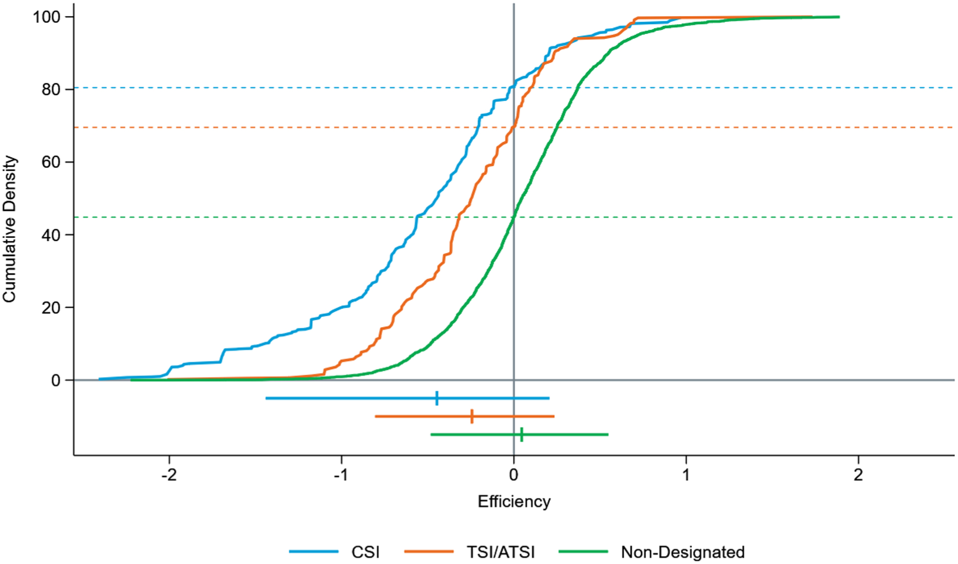
Distribution of efficiency by accountability designation (2023).
Our results thus far suggest that both CSI and TSI/ATSI schools tended to be both underfunded and inefficient. In Figure 7 we decompose the below-average outcomes of designated schools into the portion of outcomes that is attributable to underfunding versus inefficiency, which we also interpret as the portions that could be addressed through increased funding versus improved efficiency (i.e., better use of existing funding/resources). We found that 29% of CSI school underperformance could be addressed through improving their efficiency levels to the statewide average. This means that 71% of the underperformance of CSI schools would have to be addressed through increased funding if the goal were the statewide average outcome level. Even reaching the low-outcome goal of −0.5 would require addressing the underfunding of CSI schools after addressing their inefficiency that exceeded the statewide average. In other words, if the collective level of efficiency in CSI schools improved to average, they still would be performing ~1.25 SDs below the state average and 0.75 SDs below the lower-outcome target, on average. Without additional resources, the performance gains that could be expected in CSI schools are limited, and it is unlikely that these schools would meaningfully improve.

Decomposing the underperformance of designated schools by accountability designation (2023).
Even though inefficiency was less of a problem for TSI/ATSI schools on an absolute level, a larger share of underperformance in TSI/ATSI schools can be attributed to inefficiency (37%) compared with CSI schools (29%). If TSI/ATSI schools addressed inefficiency to the point where they collectively performed at average efficiency levels, they would, on average, exceed the low-outcome performance target but still would perform ~0.4 SDs below the statewide average outcome level. To meet statewide average outcomes, funding would be necessary to support this additional 63% of the average outcome shortfall experienced by TSI/ATSI schools. By contrast, nondesignated schools already exceeded the statewide average as a group. Therefore, they collectively did not have issues of underfunding or inefficiency that they needed to overcome to meet the statewide average outcome target.
Although CSI and TSI/ATSI schools tended to be both underfunded and relatively inefficient, on average, there was variation across these schools in the degree to which these two factors (underfunding and inefficiency) might be driving underperformance. Figure 8 illustrates that schools receiving accountability designations could vary drastically in terms of the extent to which efficiency and underfunding contributed to their observed outcomes. Because the majority of CSI and TSI/ATSI schools were underfunded and/or inefficient, we defined our groups to focus on schools that were underfunded (having negative funding gaps) and inefficient (having negative efficiency). As such, Efficiency Group A denotes schools with above-average efficiency, whereas Efficiency Groups B–E are increasingly inefficient. Similarly, funding Group 5 represents schools with a positive funding gap, meaning that actual spending exceeds the amount needed to achieve statewide average outcomes, and funding gaps for funding Groups 1–4 are negative, with funding Group 1 having the greatest degree of underfunding. Figure 8 show the percentages of students enrolled in schools according to Efficiency Group and funding Group broken out by accountability designation.

Percentage of students enrolled in schools by efficiency and funding group by accountability designation (2023).
We found that almost half (46%) of students in CSI schools were in schools that were severely underfunded, represented by funding Group 1. Of the CSI students represented in funding Group 1, a sizable share also attended very inefficient schools—13.1% of students in CSI schools are represented in funding Group 1 and Efficiency Group E (the most inefficient group). However, a sizable share of CSI students represented in funding Group 1 attended schools with above-average efficiency—12.6% of all CSI school students are represented in funding Group 1 and Efficiency Group A. Another ~9% of CSI school students attended schools that were very inefficient but were either only slightly underfunded or not underfunded at all (Efficiency Group E with funding Groups 4 and 5).
Although CSI school students tended to be concentrated in schools that were in either funding Group 1 or Efficiency Group E, this was not the case for students in TSI/ATSI schools. In fact, the most common pairings of Efficiency Group and funding Group for TSI/ATSI schools were funding Group 5 (sufficient funding) paired with Efficiency Groups C or E (moderate or low efficiency) and Efficiency Group A (above-average efficiency) paired with funding Groups 1–4 (very underfunded to slightly underfunded). Only a relatively small share of students in TSI/ATSI schools attended schools that were both very inefficient and very underfunded. Lastly, in contrast to the designated schools, students in nondesignated schools typically attended schools in higher efficiency and more sufficiently funded groups.
Discussion
Under ESSA, federal accountability has sought to focus improvement efforts on a relatively narrow set of the lowest-performing schools in each state. By focusing on the lowest-performing schools, the intent was to allow state and local education agencies to target limited resources to the schools most in need (Le Floch et al., 2024a). Paired with provisions in ESSA designed to ensure that additional fiscal resources are distributed to schools designated as low performing under the accountability system, the goal was to facilitate conditions that would enable the lowest-performing schools to make meaningful improvements. Thus far, limited research has been conducted examining whether schools receiving accountability designations have improved under ESSA. However, a study of Ohio’s CSI schools showed that performance in these schools may have declined during the early implementation of ESSA (Atchison et al., 2025a).
One possible reason for a lack of meaningful improvement among CSI schools is a misalignment between the level of need and challenges that these schools face and the additional resources they are provided to address those needs. Across measures of test performance, absenteeism, and graduation, CSI school performance was substantially lower than the performance of typical nondesignated schools. CSI schools also were much more likely to have higher poverty rates and enroll higher percentages of students with disabilities, who are English learners, and who are Black or Hispanic compared with nondesignated schools. This is not unique to Ohio. Le Floch et al. (2024b) found that CSI schools were more than twice as likely to have a high percentage of students in poverty or students of color compared with all public schools. However, it is important to acknowledge that the difference in performance levels and the needs of students between CSI and nondesignated schools is vast.
In contrast, the additional funding provided to CSI schools is meager. Our analysis of school-improvement funding indicated that CSI schools in Ohio, by their second and third year of designation, received about $400 per pupil in school-improvement funding. Analyzing school-level expenditures, we also estimated that spending in CSI schools increased by ~$300 to $400 per pupil in the third to fifth years of designation. Relative to average spending per pupil of ~$20,000 in Ohio’s CSI schools in 2023, these amounts of additional funding/spending only amounted to a 2% increase. The alignment between the level of school-improvement funding and additional spending amounts suggests that any additional spending is largely attributable to federal school-improvement funding and that there is little attempt to provide additional state and local resources to CSI schools. These findings are consistent with a national analysis by Blair et al. (2025), who found that school-improvement funding typically amounted to between $100 and $500 per pupil and that additional spending in CSI schools amounted to just over $300 per pupil.
Using a novel application of cost-function modeling, we estimate that, collectively, CSI schools would need to spend ~$10,000 more per pupil to meet a statewide average outcome level or ~$5,500 more per pupil to achieve a lower outcome level that still would represent meaningful improvement for these schools. These amounts are aligned with (but on the low end of) the range of additional funding needed for CSI schools from Blair et al. (2025), who found that additional spending in CSI schools likely would have to be between $8,046 and $21,452 per pupil to achieve the non-CSI mean outcome. Although we used a cost-function approach, Blair et al. (2025) based their estimates on extrapolating the relationships between student achievement and additional spending from Jackson and Mackevicius (2021), as well as the additional expected achievement gains from accountability-based school turnaround policies from Schueler et al. (2021). One possible reason for our cost estimates based on cost-function modeling being on the lower end of the range estimated by Blair et al. (2025) is the assumption that schools operate at an average level of efficiency when predicting costs from the cost-function model.
Extending the findings from the cost-function model, we were able to calculate the efficiency level of each school, defined as the difference between actual and expected student outcomes. The results of this analysis indicated that, on average, CSI schools are inefficient relative to nondesignated schools. As such, both underfunding and inefficient use of funding contribute to the low performance of CSI schools and should be addressed in efforts to improve. In decomposing CSI school underperformance, we found that ~30% of underperformance (relative to a target of statewide average performance) was due to inefficiency, with the remaining 70% the result of underfunding. As such, we contend that attempting to address inefficiency alone without additional resources will only get CSI schools so far in terms of demonstrating meaningful improvement. Without additional resources, it is likely that these schools will remain among the lowest-performing schools.
We also believe that understanding the extent to which each school’s underperformance is an issue of underfunding versus inefficiency could help state and local education agencies tailor the types of supports they provide to individual schools. Ohio’s CSI schools generally fall into three buckets: (a) both underfunded and inefficient, (b) underfunded but relatively efficient, and (c) inefficient but only slightly or not at all underfunded. Addressing inefficiency may involve additional monitoring of progress on student outcomes as well as reviews or audits of resource use and the alignment of resource use with needs. In addition, addressing inefficiency may involve more direct provision of technical assistance and short-term investments in building the capacity of staff through professional development. Underfunding, by contrast, suggests a misalignment between the level of services that schools are able to provide and the needs of students. As our findings demonstrate, CSI schools serve a very high-need student population in terms of poverty, students with disabilities, and English learners. For most CSI schools, appropriately addressing the needs of their students requires additional resources.
Although our study highlights the strong need for additional resources in schools designated as low performing under accountability, it is also paramount that any additional funding be used well. Providing substantial increases in funding to schools that have demonstrated that they do not have the capacity to use their existing resources well may not be a good investment of public dollars. As such, substantial increases in investment in low-performing schools necessarily should come with some strings attached to improve the likelihood that resources are used well along with consequences for not improving. Investments in these schools should be accompanied by sufficient technical assistance to ensure that the schools have support in building their capacity to use funding well and in ways that are likely to improve outcomes. These investments also would necessitate additional monitoring of resource use, that is, collecting information on implementation of programs and sufficient data to evaluate the effectiveness of programming. Ultimately, if substantial investments are made and appropriate supports are provided to facilitate conditions in which improvements in performance are expected, schools should be held accountable for demonstrating results with clear and meaningful consequences.
In addition to the findings herein with respect to the underfunding and inefficiency of schools designated through Ohio’s accountability system, we present a framework to evaluate the level of funding required by low-performing schools to make meaningful improvement and whether these schools are efficient in their use of the existing level of resources. We believe that rigorous estimation of underfunding and inefficiency at the school level can provide valuable information to policymakers and practitioners that could facilitate better targeting of supports and resources to the schools that need them the most.
Supplemental Material
sj-docx-1-ero-10.1177_23328584261419108 – Supplemental material for School Accountability, Underfunding, and Inefficiency
Supplemental material, sj-docx-1-ero-10.1177_23328584261419108 for School Accountability, Underfunding, and Inefficiency by Drew Atchison and Damon Blair in AERA Open
Footnotes
Acknowledgements
We are grateful to the Bill & Melinda Gates Foundation and the Ohio Department of Education and Workforce for supporting this study. The opinions expressed are those of the authors.
Declaration of Conflicting Interests
The authors declare no potential conflicts of interest with respect to the research, authorship, and/or publication of this article.
Funding
This project was funded through a grant from the Bill & Melinda Gates Foundation.
Open Practices
1.
An equitable distribution of resources is also necessary for the perception of fairness of accountability systems. Scholars have noted that where allocation of resources is inequitable, holding schools accountable for student outcomes is unfair and sets up schools serving high-need student populations for failure (Darling-Hammond, 2007; Powers, 2004).
2.
Due to the COVID-19 pandemic, CWIFT data for 2020 were not released. We estimated the 2020 values by averaging each district’s CWIFT data from 2019 and 2021.
3.
TSI/ATSI schools were excluded from this analysis. To account for districtwide trends in spending and the fact that CSI schools are overrepresented in some districts, we first centered spending by district and year by subtracting districtwide per pupil spending from each school’s per pupil spending by year. For the purpose of centering, we grouped charter schools into 16 quasi-districts according to the state’s geographic regions.
4.
![]() conducted a regression discontinuity (RD) study examining the impact of CSI designation in Ohio. Although RD represents a rigorous causal impact design, it also has limitations. In particular, the set of comparison schools near the cutoff score for designating CSI schools was made up almost entirely of TSI schools, which also received school-improvement funds. As such, there is no feasible way to compare CSI schools with nondesignated schools using RD. Using RD, Atchison et al. (2025a) found small and statistically insignificant differences in spending between CSI and non-CSI schools.
conducted a regression discontinuity (RD) study examining the impact of CSI designation in Ohio. Although RD represents a rigorous causal impact design, it also has limitations. In particular, the set of comparison schools near the cutoff score for designating CSI schools was made up almost entirely of TSI schools, which also received school-improvement funds. As such, there is no feasible way to compare CSI schools with nondesignated schools using RD. Using RD, Atchison et al. (2025a) found small and statistically insignificant differences in spending between CSI and non-CSI schools.
5.
School enrollment categories were defined as follows: <300, 300–499, 500–799, 800–1,199, and ≥1,200 students.
6.
Population-density categories were defined as follows: <100 people per square mile, 100–399, 400–799, 800–1,499, 1,500–2,999, and ≥3,000 people per square mile.
7.
The Hansen J test of overidentifying restrictions has a value of 3.178 and a p value of .075. Following the standard approach to cost-function modeling, we used multiple instruments (e.g., Duncombe et al., 2003; Taylor et al., 2018). That said, we tested a model where we omitted ZIP Code–level educational attainment as an instrument. The resulting cost model predictions were correlated with the cost predictions from the preferred model with a correlation coefficient >.999.