Sage Journals: Discover world-class research

Abstract

Recessions may disproportionally affect school districts, especially with established fiscal institutions and policies including balanced budget requirements, tax and expenditure limitations, and school finance reforms. Analyzing the Great Recession and school districts in the United States between 2003 and 2016, we estimated difference-in-differences models leveraging variation in state recession severity to evaluate revenue and expenditure impacts as well as to measure differential recession effects for districts exposed to and not exposed to fiscal institutions and policies. Although revenues and expenditures increased relative to pre-recession levels in all districts, increases were much larger in school districts with less severe than more severe recessions. Balanced budget requirements exacerbated recession effects for low-income districts, and local tax and expenditure limitations intensified recession effects for high-income districts. School finance reforms worsened recession effects for all districts. Our findings can aid districts in understanding potential recessionary impacts, given their prior established fiscal policies and institutions.

Keywords

balanced budget requirements econometric analysis economics of education educational policy equity evaluation finance fiscal institutions policy policy analysis quasi-experimental analysis recession regression analyses school finance reform tax and expenditure limitations

Introduction

The Great Recession was an 18-month economic decline that severely affected state and local government finances (T. M. Gordon, 2012; Langley, 2016; Leachman et al., 2017; Rueben et al., 2018). In elementary and secondary school districts, the Great Recession affected students, who experienced increases in class sizes, reductions in instructional time, and lower academic performance, and teachers, who experienced reductions in compensation, changes to critical elements of collective bargaining agreements, and even loss of employment entirely (Jackson et al., 2021; Strunk & Marianno, 2019). In terms of school district finances, researchers have found that the recession primarily reduced state funding for low-income school districts. Local revenues, on the other hand, were seen as a stable income source that could be increased to offset reductions in state aid, particularly in high-income school districts. Consequently, prior research has argued that total spending declined in low-income school districts, although it stayed largely unchanged in high-income school districts (Baker, 2014; Chakrabarti et al., 2014, 2015; Evans et al., 2019; Leachman, 2019; Oliff & Leachman, 2011; Shores & Steinberg, 2019b). Concerns have been raised, however, regarding this initial scholarship’s investigating a short time frame for determining impacts, offering too strong methodological assumptions, and lacking comprehensive explanations for variation in recession impacts between school districts (Barnum, 2020; Jackson et al., 2021; Swain & Redding, 2019).

We argue that the Great Recession did enduring, not just short-term, damage to school district finances, which was compounded by the framework of fiscal institutions and policies imposed on districts. Among the most prominent of fiscal institutions that might have constrained financial recovery were state-level balanced budget requirements (BBRs), which may have restricted deficit spending (Hou & Smith, 2010; Kioko & Lofton, 2021), and tax and expenditure limitations (TELs), which restricted growth of revenues and spending for local and state governments (Downes & Figlio, 2015; Mullins & Wallin, 2004). The presence of these institutions established a financial framework that could have put a formal constraint on the fiscal discretion of districts. Yet some fiscal policies, such as school finance reforms (SFRs), which created greater transfers of state aid to low-income school districts to make school funding more equitable (Corcoran & Evans, 2015; Yinger, 2004), mandated more funding to certain types of districts. This centralization of revenues could have created more dependence on state aid and potentially more vulnerability to budget cuts during recessions (Baker, 2014; Jackson et al., 2021). Because districts often responded to recessionary shocks with reductions to budgets, we examine how school districts were differentially affected, given their framework of fiscal institutions and policies, which could have encouraged and discouraged recovery efforts.

We used panel data from 2003¹ to 2016 to estimate difference-in-differences models that compared school district budgets before and after the recession (first difference) and school districts located in states with severe and less severe recessions (second difference). This approach allowed us to estimate the counterfactual—what would have happened to school districts’ budgets if the Great Recession had been less severe. Prior studies have primarily used deviations from trends or pre- and post-comparisons to measure recession effects (Chakrabarti et al., 2014, 2015; Leachman, 2019; Oliff & Leachman, 2011). In contrast, our difference-in-differences models controlled for changes in district budgets that would have occurred under a less severe economic decline and avoided the assumption that district finances would have increased at the same rate for many fiscal years.

To determine the treatment and control group, we used the State Coincident Index (SCI), maintained by the Federal Reserve Bank of Philadelphia, and an algorithm developed by Bry and Boschan (1971; see also Buerger, 2021). The data and the algorithm have been extensively used in the literature to define recessions (Crone & Clayton-Matthews, 2005; Harding & Pagan, 2003; King & Plosser, 1994; Owyang et al., 2005; Stock & Watson, 1989). We measured recessions at the state level, as all fiscal institutions in our study were enacted at the state level and influenced mainly state transfers to school districts.² For local TELs, which were more likely to influence local revenues, we provided extensive sensitivity checks employing an alternative recession definition based on county-level employment rates that confirmed our main results and that were similar to those of prior studies employing the same empirical strategy (Shores & Steinberg 2019a, 2019b). Using interaction terms, we estimated the differential effect of fiscal institutions and policies on recession impacts. For all analyses, we evaluated low- and high-income school districts to account for differences in local tax bases that influenced state and local revenues. We defined low-income districts as those in the first income quintile of their state’s distribution of school district median household income, according to the U.S. Census Bureau in 2000; we defined high-income districts as those in the last income quintile of their state’s distribution of median school district household income.

We found that revenues and expenditures grew, but much more in school districts with less severe recessions than in districts with severe recessions. For state aid, growth varied between $366 and $650 per pupil 3–7 years after the start of the economic decline for all districts. Disparities in growth for local revenues were $2,255 per pupil 8 years after the start of the recession, when low-income districts with severe and with less severe recessions were compared. Total spending per pupil also grew more in districts with less severe than severe recessions, but this disparity was $201 per pupil greater for low-income school districts relative to high-income school districts 8 years after the recession.

The presence of certain fiscal institutions exacerbated these impacts. In low-income districts, recession effects on state aid were more than $1,355 per pupil greater in districts with strict BBRs relative to districts without or with weak BBRs 8 years after the beginning of the economic downturn. High-income districts experienced recession effects on local revenues that were $276–$961 per pupil greater in districts with local TELs compared to districts without them 2–8 years after the recession. We did not find that state-level TELs altered recession impacts on school district finances in low- or high-income districts. SFRs exacerbated recession effects on state aid in low- and high-income districts ($361–$929 per pupil over the entire post-recession period).

Overall, our findings indicate that the framework of fiscal institutions and policies played a crucial role in explaining the large differences in recession outcomes across districts as well as the large gap in recovery from these effects (Baker, 2014; Knight, 2017; Leachman et al., 2017; Swain & Redding, 2019). Governments formulate and establish fiscal institutions and policies to promote prudent financial stewardship and ensure sustainable growth across business cycles, but fiscal institutions and policies can put a formal constraint on fiscal discretion and make school districts more vulnerable to recession effects. This circumstance is especially concerning during periods of economic decline, when greater fiscal autonomy could allow for flexible fiscal policy responses (Buerger et al., 2021).

We show that differences in local wealth, measured by median household income in the district prior to the recession, were another important factor in explaining variation in recession effects and recovery from them (Leachman et al., 2017; Swain & Redding, 2019). For future recessions, policymakers could derive policies to mediate recession effects that differ in the support from revenue sources and the timing of interventions between districts for more equitable post-recession recovery.

Conceptual Framework and Hypotheses

The Great Recession, the 18-month period after December 2007, exacerbated differential reductions in school spending, mainly from employee job loss, and in student achievement (Evans et al., 2019; Shores & Steinberg, 2019a, 2019b). Shores and Steinberg (2019a) asserted that targeted approaches that factored in the recession intensity and provided additional resources to districts that were disproportionally affected by recessionary events should be pursued. Yet one unaddressed factor was the role of fiscal institutions and policies that may have also disproportionally affected recovery. Therefore, we offer two research questions to be explored in this article: (a) How did the Great Recession affect revenues and expenditures in low- and high-income school districts? and (b) How did fiscal institutions and policies shape the impact of the Great Recession on low- and high-income school district finances?

To evaluate these questions, we needed to understand how fiscal institutions and policies operate to affect the financing of school districts. Fiscal institutions and policies set the foundation for fiscal decisions by establishing rules to structure government activity (T. M. Gordon, 2008, 2012; Rose, 2010) and to restrain politicians in their financial decision-making (T. M. Gordon, 2012; Musso et al., 2008; Rose, 2006, 2010). Regarding public education, the fiscal institutions and policies commonly implemented by state governments are BBRs, TELs, and SFRs. In this section, we define each of these mechanisms and formulate hypotheses about potential recessionary impacts for districts.

Balanced Budget Requirements

BBRs are state-level constitutional or statutory adopted rules that define balanced budget as an outcome or process across the budget cycle (Kioko & Lofton, 2021). Although BBRs do not explicitly exclude certain revenue funds (e.g., capital projects fund, debt service funds, special revenue funds, and permanent funds), scholars typically apply BBRs to the revenues and expenditures reported in the general fund (Bohn & Inman, 1996; Hou, 2013; Kioko & Lofton, 2021). According to Rueben et al. (2018), who built on the classification established by Hou and Smith (2006), BBRs are classified as strict if they include any one of the following rules: (a) The governor must sign a balanced budget; (b) no deficit is allowed to be carried over into the next fiscal year or biennium; and (c) the legislature must pass a balanced budget and controls must be in place on supplementary appropriations or controls must be in place within the fiscal year to avoid deficit. Thus, for our analysis, we considered BBRs with these characteristics as strict and all other arrangements of BBRs as weak.

Researchers have found that strict BBRs increase the likelihood that states balance revenues and expenses in their general fund (Hou & Smith, 2010). This finding was usually held for operating budgets in research prior to the Great Recession (Alt & Lowry, 1994; Bohn & Inman, 1996; Crain, 2003; Hong, 2015; Mahdavi & Westerlund, 2011; Poterba, 1994; Rose, 2006; Tsai, 2014). Since 2008, states with strict BBRs have also been associated with more aggressive budget cuts and increases in taxes, but not with higher fund balances (Kioko & Lofton, 2021; Rueben et al., 2018).

Because states with strict BBRs have been found to cut state spending during recessionary periods (Rueben et al., 2018), we expected them to constrain budgets and, as a consequence, transfers to school districts. Yet this constraint could have varied along the distribution of districts. We anticipated that low-income districts, which rely more on state aid, experienced greater reductions in state aid collections than did high-income school districts when strict BBRs were in place. Therefore, our first hypothesis is as follows:

H1: During a recession, low-income school districts experienced larger reductions in state aid than did high-income school districts when strict BBRs were enacted.

Tax and Expenditure Limitations

Another fiscal institution that limits budget flexibility is TELs. States enact TELs as constitutional or statutory restrictions on government taxing and spending to be imposed at the state or local level (Mullins & Wallin, 2004). Research on the impact of state TELs on state budgets has been mixed and inconclusive. Several scholars, using a binary variable indicating the implementation of state TELs, have not found an impact on state revenues or expenses (Abrams & Dougan, 1986; Bails, 1982, 1990; Cox & Lowery, 1990; Howard, 1989; Joyce & Mullins, 1991; Kenyon & Benker, 1984; Kousser et al., 2008; Mullins & Joyce, 1996; Shadbegian, 1996). Studies using stringency indices to measure the influence of TELs on state budgets have found constraining effects on tax revenues and, in some cases, spending, but not on educational outlays (Amiel et al., 2009, 2014; Deller et al., 2021).

The relationship between state TELs and local governments, on the other hand, has had two important findings. First, evidence has suggested that state TELs could reduce aid to municipalities and school districts (Hendrick & Garand, 1991; Kim, 2017; Sun, 2014), especially during a recession (Kim & Warner, 2018), when revenue collection was constrained and states attempted to ease their own financial pressures, but other studies have rejected this claim (Mullins & Joyce, 1996; Shadbegian, 1998). Second, research has suggested that counties, school districts, and municipalities (Kim, 2017; Mullins, 2004; Wen et al., 2020) with lower tax bases were more likely to be challenged by state TELs because they had less ability to diversify revenue streams and thus relied more heavily on state aid. Building on these conceptual arguments and findings, we formulated our second hypothesis:

H2: During a recession, low-income school districts experienced greater reductions in state aid than did high-income school districts when state-level TELs were enacted.

Local-level TELs are imposed on property assessments, levy rates, revenues, or expenditures. Researchers have found that local TELs decreased and slowed growth of property tax revenues, particularly when controlling for the stringency of tax limits (Dye & McGuire, 1997; Dye et al., 2005; Lowery, 1983; Shadbegian, 1999; for literature reviews, see Downes & Figlio, 2015; McGuire, 1999; Mullins & Wallin, 2004; Park et al., 2018; Stallmann et al., 2017). Evidence of the relationship between local TELs and municipal finances during the Great Recession has indicated that cities and counties with more restrictive TELs experienced greater recession impacts and had less capacity to adjust their finances than did those with less restrictive TELs (Afonso, 2013; Jimenez, 2017; Pagano & Hoene, 2018; Park et al., 2018; Wen et al., 2020; Yang, 2017).

Although local TELs could prevent revenue and expenditure growth in school districts, enacted mechanisms could mitigate their impact. Studies have suggested that increases in state aid, circumvention of TELs through provisions for overrides, and growth in non–property tax revenue, such as fees and charges, could reduce the detrimental impacts of TELs by acquiring additional revenue, thus reducing the need for spending cuts (Downes & Figlio, 2015; O’Toole & Stipak, 2000; Shadbegian, 1999; Sun, 2014; Wen et al., 2020). Yet evidence for growth in non-tax revenues has been sparse and found only small increases in fees and charges that were unable to offset local revenue limits (Downes & Killeen, 2014). Because comprehensive data on overrides were not available, empirical verifications of their ability to circumvent local TELs were also scarce, but some indications have suggested that low-poverty jurisdictions were more likely to pass overrides relative to high-poverty jurisdictions (Lyons & Lav, 2007). As a mechanism to overcome constraints to local tax revenues, state aid has been shown to effectively offset revenue constraints for low-income districts (Corcoran & Evans, 2015; Downes & Figlio, 2015). The high reliance of high-income districts on local revenues, conversely, has made them more vulnerable to local TELs, as they have tended to spend more and increase spending at a greater rate than have other districts (Jackson et al., 2014). Based on these constraining effects of local TELs, we formulated our third hypothesis:

H3: During a recession, high-income school districts experienced greater recession impacts on local revenues than did low-income school districts when local-level TELs were enacted.

School Finance Reforms

Prior to SFRs in the 1970s, local governments provided the majority of revenues for K–12 education in the United States. Because they relied heavily on property taxes, education budgets were largely a function of local tax bases and voters’ ability and willingness to tax themselves. Consequently, large disparities in school resources arose between low- and high-income school districts (Corcoran & Evans, 2015; Yinger, 2004).

This study focuses on the second wave of finance reforms, which began with Rose vs Council for Better Education (1989). These “adequacy” court cases were driven by provisions in state constitutions that required legislatures to guarantee a minimum level of free education to all students (Lukemeyer, 2003). Induced by judicial rulings (or their threat), states typically implemented foundation plans to transfer the difference between a legislatively determined minimum level of spending and a local contribution to districts (Jackson et al., 2014; Yinger, 2004). The resulting funding schemes substantially raised state transfers to low-income districts and decreased funding disparities between low- and high-income school districts (Corcoran & Evans, 2015). Specifically, Lafortune et al. (2018) found that SFRs increased average state transfers to districts at the bottom quintile of a state’s income distribution by $954 per pupil and reduced the gap in total revenues between the bottom and top quintile districts of a state’s income distribution by $696 per pupil.

As a result of more centralized funding formulas, school district funding could have become more vulnerable to recessions for two reasons. First, state transfers were largely based on income and sales tax revenues, which had more elastic responses to economic declines (Holcombe & Sobel, 1995; Sobel & Holcombe, 1996).³ The increased dependence on elastic revenue sources could have increased the relationship between business cycles and school funding for districts with SFRs relative to districts without them (Jackson et al., 2021). Second, during recessions, state governments needed to decide which spending categories to maintain or reduce (Shores & Steinberg, 2019a). Research has shown that states were more likely to cut expenses that were transfers to lower-level governments, such as school districts, as these reductions did not directly influence their own service provision (Raudla et al., 2013). We expected these two mechanisms to be more pronounced in low-income districts because they relied more heavily on state aid after SFRs than did high-income districts (Baker, 2014; Evans et al., 2019; Jackson et al., 2021; Knight, 2017; Shores & Steinberg, 2019b). From prior scholarship, our fourth hypothesis was as follows:

H4: During a recession, SFRs exacerbated recession effects on state aid more in low-income than in high-income school districts.

Methodological Approach

This section describes our econometric approach, classifies the treatment and control group, and discusses potential trade-offs in our empirical strategy.

Econometric Approach

We employed the following two strategies. For the first research question (How did the Great Recession affect revenues and expenditures in low- and high-income school districts?), we used difference-in-differences frameworks to demonstrate empirical support. These frameworks compared district finances before and after the economic downturn (first difference) and between districts located in states with severe and less severe recessions (second difference). Thus, for districts in states with severe recessions (treatment group), we estimated the counterfactual—what would have happened to district finances if the Great Recession had been less severe—by observing trends in districts located in states with less severe recessions (control group). The identification assumption was that treated districts (with severe recessions) experienced similar changes in district finances as did districts in the control group (less severe recessions).

To answer our second research question (How did fiscal institutions and policies shape the impact of the Great Recession on low- and high-income school district finances?), we interacted the recession variable with indicators measuring the presence of fiscal institutions and polices prior to the Great Recession. These interactions measured the differential effect of the recession on district finances in states with and without strict BBRs, TELs, or SFRs. This specification assumed that the economic decline influenced district finances similarly in absence of fiscal institutions.

For both empirical strategies, we employed the following econometric techniques to overcome eventual bias. First, we leveraged the Great Recession as an exogenous shock to district finances, an approach that reduced the influence of omitted district and state characteristics (Meyer, 1995). Second, district and year fixed effects were used in all specifications to control for time-invariant state characteristics and annual shocks experienced by all districts, respectively (Greene, 2003; Wooldridge, 2009). Third, we controlled for district characteristics that influenced district finances (Eom et al., 2014; Hill & Jones, 2017; Hou, 2013; Wagner & Elder, 2007). We excluded the time-varying features of these variables because they could have been affected by the recession and, thus, could have served as dependent variables for recession effects themselves.⁴ Instead, we measured each district characteristic prior to the recession and interacted the value with a linear time trend. This strategy allowed for differential trending between districts based on varying pre-recession values of each district characteristic (Brunner et al., 2020). Fourth, our difference-in-differences frameworks controlled for any systematic disparities between states in the treatment and control groups not changing over time and shocks that were common to both groups (Angrist & Pischke, 2008; Card & Krueger, 1994). Fifth, to avoid any influence of transfers and spending associated with the American Recovery and Reinvestment Act (ARRA), we subtracted ARRA funds from all revenue and expenditure categories.⁵ Because these funds could have been associated with crowding out and the flypaper effect (N. Gordon, 2004; Hines & Thaler, 1995), we further included ARRA revenues and expenditures as control variables in all our models. We treated ARRA funds as exogenous, as they were equally distributed among states, and district transfers used existing funding formulas, which were controlled for by our fixed effects and student characteristics (Anglum et al., 2021). Our results are robust to the inclusion and exclusion of ARRA measures, confirming the validity of this empirical strategy.⁶ Finally, after presenting the results for the main specifications, we ran several tests to check for potential bias in our coefficients (Angrist & Pischke, 2008; Brunner et al., 2020).

Our empirical strategy started with estimating the following difference-in-differences model as an event study (Angrist & Pischke, 2008; Autor, 2003; Granger, 1969)⁷:

\begin{array}{l} Y_{i s t} = α_{i} + β_{t} + γ δ_{t} X_{i s 2006} + θ ARR A_{i t} + \sum_{τ = 0}^{3} λ_{- τ} R e c_{s, t - τ} \\ + \sum_{τ = 1}^{8} λ_{+ τ} R e c_{s, t + τ} + ε_{i s t} \end{array}

(1)

where Y measured per-pupil revenue or expenditure for district i in state s during year t; $α_{i}$ indicated a vector of district fixed effects; $β_{t}$ referred to a vector of year fixed effects; and X represented a vector of control variables at the state and district levels. All control variables were measured prior to the Great Recession in 2006 and interacted with a linear time trend, $δ_{t}$ . We excluded time-varying characteristics because they could have been affected by the recession (Angrist & Pischke, 2008; Brunner et al., 2020). ARRA measured per-pupil revenues and expenditures associated with ARRA at the district level.

The variable Rec switched from 0 to 1 in districts that were exposed to more severe economic declines at the state level (treatment group). In districts that were not exposed to severe recessions, the indicator variable equaled zero at all times (control group). We explain how states were sorted into treatment and control groups in the next section. The coefficients $λ_{- τ}$ and $λ_{+ τ}$ quantified the change in Y for districts in the treatment group up to 3 years before and 8 years after the recession. Both coefficients were measured relative to the control group and the last year before the recession, τ = 0, which was excluded from the analysis. More intuitively, $λ_{- τ}$ and $λ_{+ τ}$ could be interpreted as lead and lag measures of the recession, respectively (Angrist & Pischke, 2008). We censored at 3 years prior to the recession to avoid the influence of prior recessions (Anglum et al., 2021) but provide estimates for additional pre-years in Appendix D11. We did not measure recession effects after 8 years to avoid fluctuations in the number of observations. The error term was represented by $ε_{ist}$ .

The key identifying assumption in Equation (1) was that trends in Y were similar in the treatment and control groups prior to the recession. To provide evidence supporting this assumption, we evaluated the results on coefficients $λ_{- τ}$ . If these estimates were close to zero or of opposite trend, relative to the post-recession coefficients, it would be reasonable to interpret $λ_{+ τ}$ as recession effects based on the counterfactual—what would have happened to district finances if the Great Recession had been less severe.

In the next step, we interacted the recession variable with indicators measuring the presence of fiscal institutions and policies in 2006 to avoid any influence of the treatment variable on the fiscal indicators (Brunner et al., 2020; Hainmueller et al., 2019):

\begin{matrix} Y_{ist} = α_{i} + β_{t} + γ δ_{t} X_{i s 2006} + θ A R R A_{i t} \\ + 1 (F i s c a l_{s, 2006} = 0) \times \sum_{τ = 0}^{3} μ_{- τ} R e c_{s, t - τ} + 1 (F i s c a l_{s, 2006} \\ = 0) \times \sum_{τ = 1}^{8} μ_{+ τ} R e c_{s, t + τ} \\ + 1 (F i s c a l_{s, 2006} = 1) \times \sum_{τ = 0}^{3} π_{- τ} R e c_{s, t - τ} + 1 (F i s c a l_{s, 2006} \\ = 1) \times \sum_{τ = 1}^{8} π_{+ τ} R e c_{s, t + τ} + ε_{i s t} \end{matrix}

(2)

where $F i s c a l_{s, 2006} = 0$ represented the absence of a fiscal institutions and policies in 2006 and $F i s c a l_{s, 2006} = 1$ represented the presence of a fiscal institution and policies in 2006.⁸ Thus, $μ_{+ τ}$ measured recession effects for districts without and $π_{+ τ}$ for districts with specific fiscal institutions and policies. We use a Wald test to investigate whether these two coefficients differed in statistically significant ways (Cameron & Trivedi, 2005; Greene, 2003).

Identification of $μ_{+ τ}$ and $π_{+ τ}$ rested on the assumption that our dependent variables would have trended in a similar manner in districts included in the control group and districts with and without fiscal institutions and policies included in the treatment group. Although they were not directly testable, we could observe pre-recession trends $μ_{+ τ}$ and $π_{+ τ}$ . If these estimates were close to zero or of opposite trend relative to the post-recession coefficients, it would be reasonable to interpret $μ_{+ τ}$ and $π_{+ τ}$ as counterfactual recession impacts on school district finances in districts with and without fiscal institutions and policies, respectively. To account for potential variation across districts with different levels of residential income, we estimated Equations (1) and (2) separately for districts in the first and fifth quintiles of each state’s median household income distribution, as measured by the 2000 U.S. Census.

Recession Definition

We identified recessions based on the SCI, maintained by the Federal Reserve Bank of Philadelphia, and an algorithm developed by Bry and Boschan (1971; see also Buerger, 2021). First, the SCI is a monthly measure of economic activity for each state and has been identified as a reliable source to measure state-level economic activity to show great variation in business cycles between states (Crone, 2006; Owyang et al., 2005; Wagner & Elder, 2007). Second, the algorithm developed by Bry and Boschan (1971) is transparent in its calculation, closely matches the National Bureau of Economic Research’s definitions of recessions, and is still recommended and used all over the world to define economic peaks and troughs (Aastveit et al., 2016; Berge & Jordà, 2013; Colombo & Lazzari, 2020; Downes & Killeen, 2014; Harding & Pagan, 2003; King & Plosser, 1994; Layton & Banerji, 2003; Owyang et al., 2005; Stock & Watson, 1989). The algorithm developed by Bry and Boschan (1971) uses three distinct criteria for determining economic peaks and troughs. The first criterion in the algorithm determines the months before and after a focal month that is used to calculate local minima and maxima (5 months). The second criterion defines the length of up- and downturns in the economy (5 months). The last criterion determines the length of an entire business cycle (15 months).⁹

We used the SCI and the Bry and Boschan (1971) algorithm to determine a business cycle for all states in our sample. We then grouped states into low and high recession impacts if they had fewer or more than 8 recession months in one of their fiscal years during the study period. Table 1 indicates the states in the treatment and control groups. To test the validity of this strategy, we provided several checks that the recession definition was not correlated with district or state characteristics that could have also influenced district finances (see Appendix D). Moreover, we used alternative cut-off points for our recession definition (see Appendix E).

Table 1

States Grouped According to Treatment Status

Control	Treatment
Arkansas, Nebraska, New Hampshire, North Dakota, and Utah	Alabama, Arizona, California, Colorado, Connecticut, Delaware, Florida, Georgia, Idaho, Illinois, Indiana, Iowa, Kansas, Kentucky, Louisiana, Maine, Maryland, Massachusetts, Michigan, Minnesota, Mississippi, Missouri, Montana, Nevada, New Jersey, New Mexico, New York, North Carolina, North Dakota, Ohio, Oklahoma, Oregon, Pennsylvania, Rhode Island, South Carolina, South Dakota, Tennessee, Texas, Vermont, Virginia, Washington, West Virginia, Wisconsin, and Wyoming

Control

Treatment

Arkansas, Nebraska, New Hampshire, North Dakota, and Utah

Alabama, Arizona, California, Colorado, Connecticut, Delaware, Florida, Georgia, Idaho, Illinois, Indiana, Iowa, Kansas, Kentucky, Louisiana, Maine, Maryland, Massachusetts, Michigan, Minnesota, Mississippi, Missouri, Montana, Nevada, New Jersey, New Mexico, New York, North Carolina, North Dakota, Ohio, Oklahoma, Oregon, Pennsylvania, Rhode Island, South Carolina, South Dakota, Tennessee, Texas, Vermont, Virginia, Washington, West Virginia, Wisconsin, and Wyoming

Note. The table displays states in treatment and control groups according to recession definitions explained in the section Recession Definition. Alaska, Hawaii, and the District of Columbia were excluded from the analysis because of their unique economies and school systems. Of all students enrolled in school districts that were used in the analysis, 8% were in the control, and 92% were in the treatment group.

Potential Trade-Offs in the Empirical Strategy

We faced five major trade-offs. First, we lost finer-grained information on the economic activity in each state by using difference-in-differences frameworks. For example, the SCI dropped by more than 10 points in Montana, compared to 3 points in New York, from January–December 2008. Therefore, we lost the ability to identify more nuanced differences between treated states. Yet this empirical strategy enabled us to estimate a counterfactual, test for parallel trends, and measure changes in recession impacts over time. Second, the control group potentially included states that may have been exposed to some recession effects. We are still confident that we captured most of the recession effects on state budgets, given that the control group showed a decline or stagnation in revenues and expenditures only in a few fiscal years (see Figure 1 and Tables 3a–3c). Nevertheless, we assert that the coefficients attached to the recession indicator should be interpreted as conservative estimates. Third, our control group included only a few states. Consequently, it is more likely that we failed to reject the null hypothesis even though it was false and should have been rejected (false negative). Note, however, that if recession impacts on state finances were large and occurred in many states, estimates would be statistically significant at the commonly used thresholds (Cameron & Trivedi, 2005). Fourth, there could have been spillover effects from one state economy to another. This problem seemed to apply less to our analysis because researchers have found distinct business cycles for each state that differed in their timing and intensity (Hamilton & Owyang, 2012; Owyang et al., 2005). Moreover, we studied school district finances, which were based on property, sales, and income tax revenue that was unlikely to incur major spillover effects from business cycles in other states (Gruber, 2005). Finally, our state-level measures could have been correlated over time, and states could have been subject to idiosyncratic shocks. To adjust for these two problems, we clustered all standard errors at the state level (see Angrist & Pischke, 2008).¹⁰

Figure 1.

Average revenues and expenditures for districts in the treatment and control group for different samples.

Data and Sample

Several points about our sources and data are important to note. First, we employed information on school district finances from the School District Finance Survey (F-33) maintained by the National Center for Education Statistics. We preferred this information over data available from the U.S. Census Bureau, as it was more accurate in its classification of revenue sources (Goldstein & McGee, 2021).

Second, our analysis focused on state and local revenues, as the fiscal institutions and polices we were interested in were implemented at either the state or local level. Regarding school district spending, we focused solely on total expenditures per pupil. Descriptive statistics and findings for additional revenue and expenditure categories are shown in Appendix B. To avoid any influence of transfers and spending associated with ARRA, we subtracted ARRA funds from all revenue and expenditure categories and included them as controls in our models.

Third, to determine state-level business cycles, we used the SCI from the Federal Reserve Bank of Philadelphia. The index is based on four time series measures: non-farm payroll employment, average hours worked in manufacturing by production workers, the unemployment rate, and salary and wage disbursements deflated by the consumer price index, which are combined using a dynamic single-factor model (Crone, 2006; Crone & Clayton-Matthews, 2005; Stock & Watson, 1989).

Fourth, we employed the following measures of fiscal institutions and policies. We created indicators of strict BBRs based on the work of Hou and Smith (2006, 2010), Kioko and Lofton (2021), and Rueben et al. (2018). Information on state and local TELs was taken from Amiel et al. (2009), who listed the most significant changes in both fiscal institutions between 1969 to 2005, as the most comprehensive to date (Maher et al., 2016). We augmented these data with records from the Lincoln Institute of Land Policy’s Tax Limits data,¹¹ using the classification scheme developed by Amiel et al. (2009). Our SFR indicator was based on the timing of the actual court orders, as in Brunner et al. (2020). We chose this tabulation because several authors argued that the unpredictable timing of court-ordered reforms made SFRs exogenous shocks to school district budgets (Jackson et al., 2014). All fiscal indicators were measured in 2006 to avoid any influence of the recession on them (Angrist & Pischke, 2008; Brunner et al., 2020). Table 2 shows the share of states and observations being exposed to fiscal institutions. The correlation between fiscal institutions and policies was always lower than 0.25, except for strict BBRs and local TELs, which were correlated by 0.5. In robustness checks, we used alternative classifications of BBRs established by Costello et al. (2017), TELs by Mullins and Wallin (2004), and SFRs by Lafortune et al. (2018), as shown in Appendix E.

Table 2

States With Fiscal Institutions and Policies

Fiscal institution or policy	Percentage share of states implemented
Balanced budget requirement	69%
State tax and expenditure limits	60%
Local tax and expenditure limits	77%
School finance reform	45%

Finally, control variables were taken from the following data sets. First, we used school district information on total enrollment, share of White students,¹² share of students receiving free or reduced-price lunch, share of students with an individual education plan, and share of students who were English language learners from the Common Core of Data, which is provided by the National Center for Education Statistics. To address the limitations associated with the use of free and reduced-price lunch variables to gauge poverty levels in school districts (Domina et al., 2018), we incorporated a poverty measure based on the Small Area Income and Poverty Estimates by the U.S. Census Bureau. County-level employment shares in the goods-producing and services-producing industries as well as public administration jobs (federal, state, and local governments) were included as control variables. Information on simple majorities (at least above 50% of members identifying as Democrat) in the house and senate of each state’s legislature was taken from “The Book of States” published by the Council of State Governments. Fiscal information on state balances and rainy-day funds was taken from the Pew Charitable Trusts and based on “The Fiscal Survey of the States” collected by the National Association of State Budget Officers. We used data from the Annual Survey of State and Local Government maintained by the U.S. Census Bureau to measure states’ long-term debt. Descriptive statistics for all control variables are shown in Appendix A1. Because the recession was likely to influence our control variables, we measured them in 2006 and interacted them with a linear time trend to allow for differential trending of baseline state and local characteristics (Angrist & Pischke, 2008; Brunner et al., 2020). For our endogeneity checks, we employed school districts’ characteristics from the 2006 American Community Survey, such as median household income, fraction living in poverty, fraction who obtained a high school degree, and fraction with at least a bachelor’s degree.

Using these sources, we created a panel data set from 2003–2016 consisting of elementary, secondary, and unified school districts. We dropped districts in Alaska, Hawaii, and the District of Columbia from our analysis because of their unique economies, tax systems, and school finance arrangements (Hou, 2001; Wagner, 2003). We followed Brunner et al. (2020) and Lafortune et al. (2018) and excluded districts from our sample with fewer than 100 students and with high volatility in enrollment, revenues, or expenditures.¹³ Based on median household income for school districts in 2000, from the U.S. Census Bureau, we grouped districts into income quintiles in each state.

Figure 1 displays average total revenues and expenditures for school districts in the treatment and control groups for samples of all districts and districts in the lowest and highest income quintiles. Trends in all dependent variables were close to parallel for the treatment and control variables prior to the economic downturn, providing evidence that we were able to estimate the counterfactual—what would have happened to district finances in the treatment group if the recession had been less severe. It’s important to note further that the control group only displayed a few years of declining revenues or expenditures, which further supported our estimation strategy. Tables 3a–3c show means and standard deviations for our main dependent variables using different fiscal years and the same samples as shown in Figure 2. Tables that include descriptive statistics for different spending categories can be found in Appendix B.

Table 3a

Means and Standard Deviations for Per-Pupil Revenue and Expenditure Measures for All School Districts

	All districts
	Treat				Control				Difference
	2006	2010	2014	2016	2006	2010	2014	2016	2006	2010	2014	2016
Total revenue	13,353	14,182	14,287	14,501	12,395	14,135	14,342	15,040	958***	−47	55	539***
	(4,748)	(5,341)	(6,196)	(4,887)	(2,785)	(3,526)	(4,158)	(4,596)
State	6,222	6,204	6,472	6,813	5,033	5,715	5,738	5,845	1,189***	−489***	−734***	−968***
	(2,865)	(3,064)	(3,362)	(3,202)	(1,721)	(1,842)	(2,667)	(2,681)
Local	5,731	6,106	6,390	6,179	5,946	6,463	7,321	7,894	−215	357**	931***	1,715***
	(4,774)	(5,331)	(6,051)	(4,794)	(3,267)	(3,881)	(4,826)	(5,086)
Total expenditures	13,300	13,665	14,077	14,302	12,047	13,647	14,225	15,125	1,253***	−18	−148	823***
	(4,796)	(5,835)	(6,278)	(5,222)	(3,503)	(3,859)	(4,408)	(5,289)
SCI (state level)	95.74	94.73	109.4	118.8	95.35	100.1	115.8	123.6
	(0.331)	(0.613)	(0.841)	(0.92)	(0.643)	(1.19)	(1.632)	(1.786)
N	10792	10553	10656	8281	677	640	650	624

Note. The table shows means and standard deviations (in parentheses). Samples are explained in Figure 1. SCI = State Coincident Index. Differences between treatment and control group are statistically significant at the following levels: *p<0.1, **p<0.05, and ***p<0.01.

Table 3b

Means and Standard Deviations for Per-Pupil Revenue Measures and Total Expenditures for Low-Income School Districts

	Low-income school district (Quintile 1)
	Treat				Control				Difference
	2006	2010	2014	2016	2006	2010	2014	2016	2006	2010	2014	2016
Total revenue	13,214	14,102	14,143	13,786	13,284	15,209	15,426	16,156	−70	−1,107***	−1,283***	−2,370***
	(4,491)	(4,938)	(5,971)	(3,809)	(2,871)	(3,904)	(4,231)	(4,803)
State	7,341	7,394	7,668	7,760	5,342	6,004	5,992	6,127	1,999***	1,390***	1,676***	1,633***
	(2,864)	(3,254)	(4,064)	(3,152)	(1,861)	(2,010)	(2,897)	(3,037)
Local	3,984	4,308	4,640	4,017	6,119	6,696	7,763	8,324	−2,135***	−2,388***	−3,123***	−4,307***
	(3,741)	(3,793)	(4,588)	(2,740)	(3,357)	(4,091)	(5,029)	(5,173)
Total expenditures	13,117	13,564	13,954	13,583	12,792	14,378	15,241	15,904	325	−814***	−1,287***	−2,321***
	(4,516)	(5,813)	(5,857)	(4,066)	(4,556)	(3,775)	(4,592)	(4,958)
N	2909	2799	2816	1971	239	217	222	207

Note. The table shows means and standard deviations (in parentheses). Samples are explained in Figure 1. SCI only varied at the state level and did not change with the low-income school district sample. SCI = State Coincident Index. Differences between treatment and control group are statistically significant at the following levels: *p<0.1, **p<0.05, and ***p<0.01.

Table 3c

Means and Standard Deviations for Per-Pupil Revenue Measures and Total Expenditures for High-Income School Districts

	Quintile 5
	Treat				Control				Difference
	2006	2010	2014	2016	2006	2010	2014	2016	2006	2010	2014	2016
Total revenue	15,059	15,975	16,346	16,152	11,705	13,166	13,398	13,988	3,354***	2,809	2,948***	2,164***
	(5,799)	(6,600)	(7,414)	(5,454)	(2,773)	(2,779)	(3,340)	(3,704)
State	4,603	4,581	4,922	5,294	4,472	5,133	5,478	5,578	131***	−552***	−556***	−284***
	(2,606)	(2,453)	(2,558)	(2,528)	(1,322)	(1,627)	(2,321)	(2,295)
Local	9,546	10,136	10,446	9,795	6,516	6,835	7,231	7,680	3,030***	3,301*	3,215***	2,115***
	(6,116)	(7,018)	(7,740)	(6,457)	(3,394)	(3,705)	(4,280)	(4,591)
Total expenditures	15,212	15,708	15,894	15,812	11,628	12,834	13,412	14,175	3,584***	2,874	2,482***	1,637***
	(6,073)	(7,274)	(7,142)	(5,767)	(2,786)	(3,177)	(3,809)	(3,694)
N	1,371	1,371	1,371	1,371	71	71	71	71

Note. The table shows means and standard deviations (in parentheses). Samples are explained in Figure 1. SCI only varied at the state level and did not change with high-income school district sample. SCI = State Coincident Index. Differences between treatment and control group are statistically significant at the following levels: *p<0.1, **p<0.05, and ***p<0.01.

Figure 2.

Event study coefficients for total revenues and expenditures per pupil.

Results

Figure 2 and Table 4 display the results for Equation (1). According to Figure 2, districts that were exposed to severe recessions experienced less growth in total revenue compared to districts that experienced less severe recessions. This effect persisted for 2–8 years after the start of the economic downturn, with coefficient sizes of $467 per pupil and $2,366 per pupil, respectively (see Column 1 of Table 4). These results were driven by low-income districts (Quintile 1), as depicted in Panel B of Figure 2. State and local revenues contributed to the gap, but estimates were greater for local revenues in later post years. High-income districts (Quintile 5) showed sizable but smaller and imprecisely estimated disparities for all revenue measures. According to a sample of all districts, total expenditures per pupil grew less than did total revenue (see Figure 2 and Column 4 of Table 4). Once more, coefficients were larger and more precisely estimated for low-income than for high-income districts.¹⁴

Table 4

Regression Results for Per-Pupil Revenue Measures and Total Expenditures

	All districts				Quintile 1				Quintile 5
	Total revenue	Staterevenue	Localrevenue	Total expenditures	Total revenue	State revenue	Local revenue	Total expenditures	Total revenue	State revenue	Local revenue	Total expenditures
	(1)	(2)	(3)	(4)	(5)	(6)	(7)	(8)	(9)	(10)	(11)	(12)
Recession t−3	−336	−684**	213	−586	−167	−974***	535*	−519	−1,371*	−940**	−463	−1,356*
	(459)	(297)	(309)	(521)	(410)	(323)	(276)	(541)	(683)	(390)	(576)	(713)
Recession t−2	−54	−653**	494*	−268	−101	−920***	620**	−245	−702	−829**	66	−724
	(413)	(261)	(282)	(417)	(434)	(315)	(270)	(492)	(608)	(359)	(529)	(563)
Recession t−1	65	−291**	337*	−118	39	−367**	323*	−166	−209	−361*	139	−318
	(218)	(119)	(169)	(222)	(227)	(142)	(170)	(264)	(295)	(187)	(235)	(329)
Recession t+1	−135	−36	−124	−213	−152	−24	−100	−107	−41	16	−52	−130
	(151)	(140)	(114)	(204)	(112)	(140)	(126)	(145)	(216)	(168)	(156)	(347)
Recession t+2	−467**	−207	−340**	−781**	−508**	−85	−341**	−428**	−367	−169	−232	−690
	(228)	(180)	(142)	(335)	(224)	(167)	(158)	(210)	(272)	(278)	(293)	(539)
Recession t+3	−827***	−366*	−571**	−1,642***	−760**	−226	−578**	−1,359***	−566*	−356	−299	−1,019
	(221)	(216)	(221)	(318)	(318)	(219)	(254)	(327)	(288)	(335)	(392)	(616)
Recession t+4	−1,173***	−576**	−653**	−2,131***	−992**	−376	−683*	−1,949***	−831**	−648	−238	−1,328**
	(260)	(250)	(270)	(357)	(378)	(276)	(352)	(487)	(382)	(399)	(452)	(537)
Recession t+5	−1,406***	−650**	−834**	−2,191***	−1,309***	−553**	−872*	−2,227***	−1,077**	−731	−421	−1,485***
	(282)	(264)	(359)	(372)	(340)	(252)	(477)	(552)	(441)	(456)	(516)	(494)
Recession t+6	−1,656***	−615*	−1,152***	−2,398***	−1,386***	−479	−1,113*	−2,306***	−1,281**	−787	−545	−1,773***
	(360)	(306)	(406)	(426)	(412)	(320)	(570)	(547)	(569)	(535)	(607)	(580)
Recession t+7	−2,009***	−619*	−1,516***	−2,675***	−1,774***	−453	−1,545**	−2,610***	−1,668**	−1,017*	−694	−2,290***
	(401)	(354)	(436)	(483)	(432)	(400)	(647)	(569)	(653)	(574)	(648)	(706)
Recession t+8	−2,366***	−398	−2,121***	−2,921***	−2,276***	−310	−2,260***	−2,762***	−1,845**	−783	−1,129	−2,563***
	(468)	(396)	(463)	(564)	(463)	(467)	(688)	(638)	(796)	(636)	(742)	(849)
Observations	129,901	129,901	129,901	129,901	35,728	35,728	35,728	35,728	17,067	17,067	17,067	17,067
R-squared	0.3	0.2	0.2	0.1	0.2	0.1	0.1	0.1	0.2	0.1	0.1	0.1

Note. The samples are described in Figure 1 and Table 1. Estimates were based on event study models described in Equation 1. Each column presents results for separate regressions, where the dependent variable is listed on top of each column. All specifications included (a) controls for district characteristics, (b) state-level fiscal institutions, (c) states’ political characteristics, and (d) state and fiscal year fixed effects. All standard errors are clustered at the state level and displayed in parentheses.

p<0.1. ** p<0.05. *** p<0.01.

Tables 5 –8 display the results for Equation (2). Note that the difference column indicates statistically significant differences between districts with and without fiscal institutions that are at least at the 5% level.¹⁵ Following our hypotheses, we solely present results for high- and low-income school districts (Appendix C shows all districts). We used state and local revenues as dependent variables,¹⁶ even if institutions targeted only one of these revenue sources, to analyze whether districts could offset reductions in one revenue source over another. We further display estimates for models with total expenditures as the dependent variable.

Table 5

Regression Results for Strict Balanced Budget Requirements

	t−3	t−2	t−1	t+1	t+2	t+3	t+4	t+5	t+6	t+7	t+8
Quintile 1
Panel A: State revenue
No strict BBR	−734**	−799**	−212	179	312	109	−60	−182	−5	142	362
	(279)	(310)	(199)	(189)	(203)	(291)	(298)	(326)	(393)	(474)	(541)
Strict BBR in place	−945***	−887***	−420***	−166	−396*	−624**	−823**	−1,052***	−1,099**	−1,113**	−993*
	(294)	(247)	(109)	(121)	(209)	(283)	(381)	(369)	(415)	(451)	(521)
Difference	211	88	208	345	708***	733***	763***	870***	1,094***	1,255***	1,355***
Panel B: Local revenue
No strict BBR	482	558*	215	−162	−384**	−568**	−647*	−898*	−1,245**	−1,783***	−2,304***
	(314)	(330)	(185)	(117)	(164)	(253)	(362)	(469)	(552)	(629)	(695)
Strict BBR in place	570*	686**	403**	−62	−295*	−551**	−670*	−816*	−998*	−1,387**	−2,200***
	(290)	(263)	(186)	(131)	(162)	(249)	(339)	(451)	(547)	(633)	(677)
Difference	−88	−128	−188	−100	−89	−17	23	−82	−247	−396*	−104
Panel C: Total expenditures
No strict BBR	−547	−444	−320	34	−62	−1,609**	−1,824***	−2,203***	−2,147***	−2,413***	−2,473***
	(520)	(535)	(328)	(242)	(353)	(430)	(455)	(456)	(528)	(564)	(634)
Strict BBR in place	−432	−119	−86	−187	−647***	−1,585***	−2,140***	−2,372***	−2,548***	−2,864***	−3,055***
	(439)	(365)	(214)	(135)	(232)	(381)	(570)	(625)	(607)	(616)	(693)
Difference	−115	−325	−234	221	585	489	316	169	401	451	582
Quintile 5
Panel D: State revenue
No strict BBR	−841	−769	−236	129	−48	−324	−648	−574	−594	−829	−545
	(553)	(512)	(255)	(236)	(311)	(455)	(488)	(496)	(589)	(669)	(732)
Strict BBR in place	−875**	−783**	−397*	−94	−344	−535	−839**	−1,011**	−1,065*	−1,248**	−1,004*
	(397)	(350)	(211)	(205)	(370)	(394)	(410)	(445)	(533)	(504)	(556)
Difference	34	14	161	223	296	211	191	437	471	419	459
Panel E: Local revenue
No strict BBR	−343	383	204	148	95	−42	26	22	−380	−420	-804
	(579)	(642)	(289)	(128)	(241)	(386)	(535)	(564)	(651)	(678)	(779)
Strict BBR in place	−372	145	272*	−231	−492	−621*	−555	−730	−725	−1,006	−1,417**
	(563)	(344)	(152)	(178)	(296)	(341)	(430)	(552)	(636)	(722)	(826)
Difference	29	238	−68	379**	587***	579**	581	752**	345	586	613
Panel F: Total expenditures
No strict BBR	−986	−439	−262	58	−74	−695	−1,009	−948	−1,223	−1,698	−2,097*
	(724)	(626)	(334)	(474)	(572)	(731)	(790)	(767)	(821)	(1,032)	(1,186)
Strict BBR in place	−1,265*	−584	−189	−338	−1,205**	−1,454**	−1,759***	−1,960***	−2,237***	−2,741***	−2,885***
	(752)	(546)	(315)	(320)	(576)	(641)	(558)	(522)	(562)	(648)	(774)
Difference	279	145	−73	396	1,131*	759	750	1,012	1,014	1,043	788

Note. Strict BBRs have the following characteristics: (a) The governor must sign a balanced budget; (b) no deficit is allowed to be carried over into the next fiscal year or biennium; and (c) the legislature must pass a balanced budget accompanied by controls in place on supplementary appropriations or controls in place within the fiscal year to avoid deficit. Sample, control variables, and statistical significance are presented as stated in Figure 1 and Table 1. Estimates were based on event study models described in Equation (2). Gray shaded areas indicate statistically significant differences between districts with and without the fiscal policy. Dependent variables are defined for each panel separately. All standard errors are clustered at the state level and displayed in parentheses. BBR = balanced budget requirement.

p<0.1. ** p<0.05. *** p<0.01.

Table 6

Regression Results for State Tax and Expenditure Limitations

	t−3	t−2	t−1	t+1	t+2	t+3	t+4	t+5	t+6	t+7	t+8
Quintile 1
Panel A: State revenue
No state TEL	−914***	−1,004***	−391**	180	54	−167	−212	−351	−354	−282	−48
	(317)	(304)	(173)	(222)	(251)	(272)	(269)	(316)	(364)	(489)	(530)

State TEL in place	−987***	−822***	−320**	−143	−169	−284	−495	−674**	−585	−609	−523
	(350)	(297)	(131)	(112)	(167)	(241)	(321)	(294)	(355)	(431)	(512)
Difference	73	−182	−71	323	223	117	283	323	231	327	475
Panel B: Local revenue
No state TEL	298	360	122	−144	−321*	−505*	−516	−795*	−1,021*	−1,616**	−2,266***
	(294)	(216)	(115)	(106)	(117)	(258)	(359)	(443)	(535)	(618)	(684)
State TEL in place	663**	843***	496***	−87	−359**	−661***	−837**	−954**	−1,233**	−1,597**	−2,332***
	(259)	(246)	(197)	(119)	(144)	(235)	(321)	(438)	(532)	(618)	(663)
Difference	−365	−483**	−374**	−57	38	156	321	159	212	−19	66
Panel C: Total expenditures
No state TEL	−658	−499	−313	109	23	−971***	−1,541***	−1,893***	−1,956***	−2,381***	−2,522***
	(609)	(513)	(315)	(240)	(287)	(334)	(423)	(461)	(491)	(549)	(619)
State TEL in place	−479	−58	−44	−253*	−705***	−1,660***	−2,286***	−2,493***	−2,615***	−2,875***	−3,020***
	(444)	(359)	(214)	(137)	(231)	(380)	(539)	(577)	(568)	(585)	(663)
Difference	−179	−441	−269	362	728**	689*	745**	600*	659*	494	498
Quintile 5
Panel D: State revenue
No state TEL	−1,193**	−1,025*	−357	179	−51	−400	−594	−707	−1,053*	1,345***	−1,112
	(564)	(520)	(239)	(192)	(257)	(381)	(501)	(573)	(563)	(641)	(669)
State TEL in place	−800**	−747**	−392*	−9	−99	−196	−543	−540	−490	−798	−601
	(389)	(327)	(203)	(206)	(363)	(413)	(417)	(459)	(544)	(519)	(564)
Difference	−393	−278	35	188	48	−204	−51	−167	−563*	−547	−511
Panel E: Local revenue
No state TEL	−698	−129	44	−81	−233	−224	26	−166	−213	−393	−829
	(528)	(448)	(189)	(193)	(332)	(425)	(512)	(542)	(555)	(630)	(697)
State TEL in place	−43	564	452**	−120	−354	−572	−598	−651	−795	−902	−1,276*
	(484)	(352)	(210)	(165)	(296)	(381)	(459)	(508)	(589)	(623)	(709)
Difference	−655	−693*	−408**	39	121	348	624	485	582	509	447
Panel F: Total expenditures
No state TEL	−1,624**	−907	−204	−45	−277	−677	−751	−937	−1,328	−2,144*	−2,515**
	(690)	(602)	(379)	(388)	(541)	(790)	(848)	(844)	(853)	(1,074)	(1,170)
State TEL in place	−942	−310	−171	−280	−1,011*	−1,319**	−1,712***	−1,679***	−1,917***	−2,315***	−2,559***
	(709)	(520)	(339)	(365)	(587)	(605)	(520)	(492)	(573)	(678)	(798)
Difference	−682	−597	−33	235	734	642	961	742	589	171	44

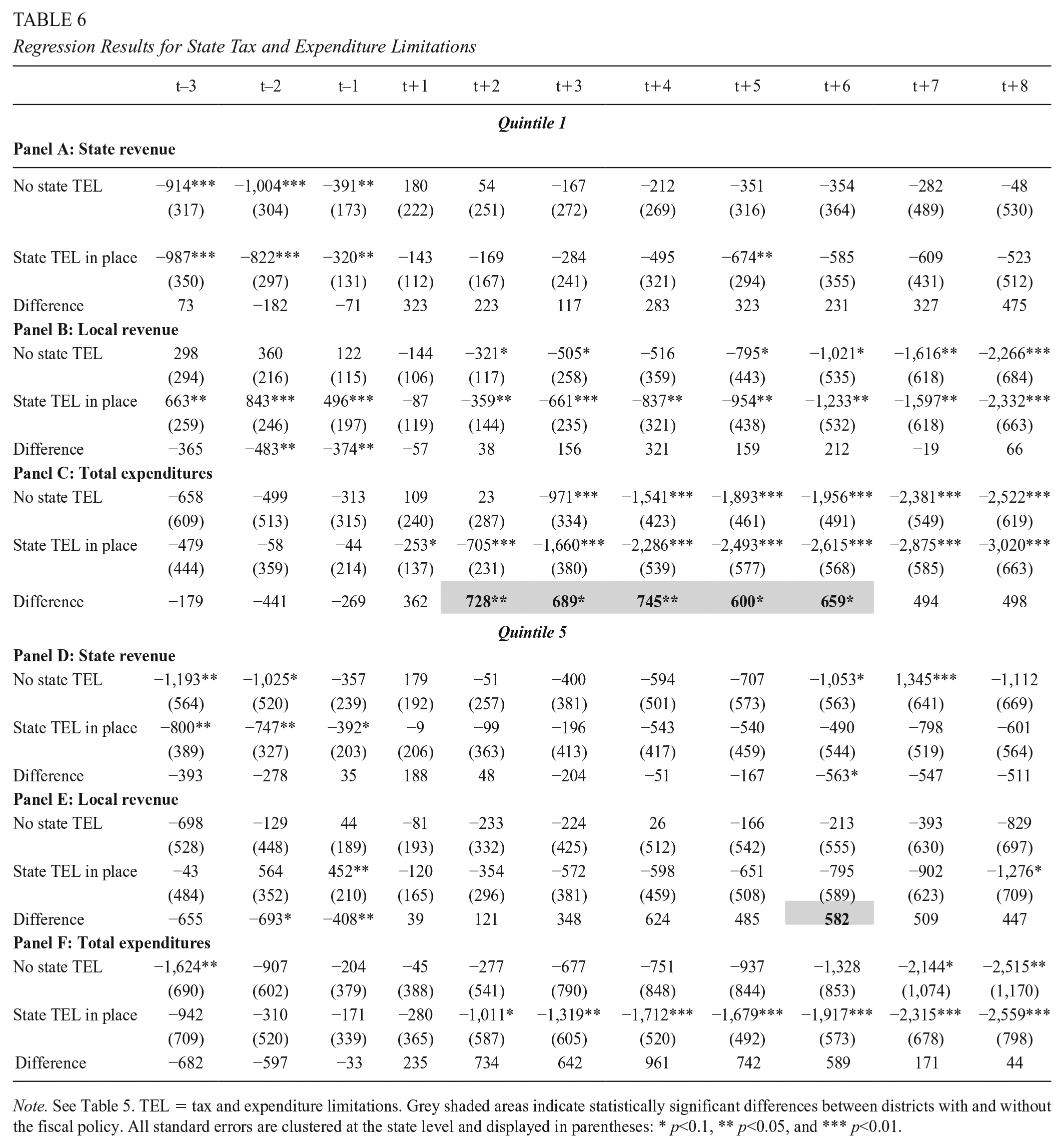
Note. See Table 5. TEL = tax and expenditure limitations. Grey shaded areas indicate statistically significant differences between districts with and without the fiscal policy. All standard errors are clustered at the state level and displayed in parentheses: * p<0.1, ** p<0.05, and *** p<0.01.

Table 7

Regression Results for Local Tax and Expenditure Limitations

	t−3	t−2	t−1	t+1	t+2	t+3	t+4	t+5	t+6	t+7	t+8
Quintile 1
Panel A: State revenue
No local TEL	−1,034***	−1,190***	−413***	619**	525	304	109	153	353	567	967
	(373)	(251)	(99)	(258)	(318)	(324)	(325)	(445)	(482)	(596)	(685)
Local TEL in place	−619**	−566***	−215**	−141	−193	−357	−510	−691**	−675*	−690*	−473
	(239)	(186)	(84)	(94)	(159)	(234)	(322)	(286)	(336)	(395)	(442)
Difference	−415	−624	−198**	760***	718**	661**	619**	844**	1,028***	1,257***	1,440***
Panel B: Local revenue
No Local TEL	36	165	−132	−338***	−549**	−695**	−759*	−946*	−1,103*	−1,679**	−2,073***
	(357)	(238)	(131)	(104)	(205)	(266)	(390)	(484)	(604)	(696)	(769)
Local TEL in place	796***	875***	484**	−28	−311**	−585**	−698**	−871*	−1,135**	−1,551**	−2,294***
	(266)	(246)	(186)	(117)	(143)	(241)	(333)	(458)	(552)	(640)	(697)
Difference	−760*	−710**	−616**	−310*	−238	−110	−61	−75	32	−128	221
Panel C: Total expenditures
No local TEL	−1,141**	−1,025***	−739***	560*	609	−312	−1,002*	−1,477***	−1,498**	−1,873***	−1,885***
	(525)	(288)	(170)	(314)	(529)	(548)	(506)	(508)	(613)	(670)	(691)
Local TEL in place	56	298	116	−209	−565***	−1,457***	−1,956***	−2,132***	−2,274***	−2,610***	−2,730***
	(286)	(229)	(177)	(141)	(201)	(331)	(497)	(513)	(513)	(570)	(652)
Difference	−1,197***	−1,323***	−855***	769**	1,174**	1,145***	954***	655	776*	737**	845**
Quintile 5
Panel D: State revenue
No local TEL	−831	−729	−187	127	−213	−634	−835*	−597	−654	−675	−344
	(696)	(632)	(290)	(245)	(290)	(416)	(475)	(511)	(556)	(697)	(793)
Local TEL in place	−241	−248	−97	−84	−239	−388	−518	−591	−546	−676	−344
	(447)	(430)	(262)	(193)	(339)	(428)	(400)	(443)	(525)	(568)	(636)
Difference	−590	−481	−90	211	26	−246	−317	−6	−108	1	0
Panel E: Local revenue
No local TEL	−339	146	38	134	63	26	336	318	230	264	43
	(543)	(455)	(165)	(183)	(310)	(433)	(514)	(559)	(636)	(732)	(810)
Local TEL in place	38	555*	433**	−158	−429	−611*	−596	−631	−693	−838	−1,157
	(512)	(316)	(172)	(152)	(266)	(354)	(454)	(516)	(586)	(649)	(740)
Difference	−377	−409	−395*	292**	492**	637**	932**	949***	923***	1,102***	1,200***
Panel F: Total expenditures
No local TEL	−1,143	−600	−284	193	−38	−482	−526	−414	−698	−1,248	−1,427
	(786)	(653)	(365)	(451)	(471)	(957)	(1,087)	(1,015)	(1,077)	(1,365)	(1,513)
Local TEL in place	−923	−313	−103	−299	−1,014*	−1,357**	−1,679***	−1,696***	−1,892***	−2,360***	−2,526***
	(732)	(540)	(309)	(317)	(583)	(611)	(499)	(506)	(572)	(682)	(841)
Difference	−220	−287	−181	492	976**	875	1,153	1,282	1,194	1,112	1,099

Table 8

Regression Results for School Finance Reforms

	t−3	t−2	t−1	t+1	t+2	t+3	t+4	t+5	t+6	t+7	t+8
Quintile 1
Panel A: State revenue
No SFR	−493**	−424**	−206	150	82	37	−202	−295	−150	−21	115
	(243)	(191)	(179)	(159)	(189)	(255)	(264)	(276)	(347)	(433)	(490)
SFR in place	−892***	−852***	−390**	−211*	−284	−582**	−650*	−844***	−863**	−950**	−715
	(290)	(269)	(147)	(110)	(171)	(241)	(349)	(292)	(348)	(412)	(477)
Difference	339*	428**	184	361**	366*	619***	448*	549**	713**	929***	830**
Panel B: Local revenue
No SFR	721***	772***	153	−138	−348**	−529**	−536	−774*	−1,158**	−1,694***	−2,250***
	(200)	(216)	(148)	(89)	(153)	(247)	(345)	(427)	(521)	(607)	(688)
SFR in place	875***	978***	569**	−66	−360**	−682***	−852***	−926**	−1,043**	−1,427**	−2,274***
	(239)	(233)	(219)	(113)	(149)	(234)	(308)	(421)	(507)	(615)	(666)
Difference	−154	−206	−416**	−72	12	153	316**	152	−115	−267	24
Panel C: Total expenditures
No SFR	178	314	−144	−61	−273	−1,128***	−1,642***	−1,918***	−2,073***	−2,330***	−2,423***
	(349)	(271)	(361)	(243)	(304)	(350)	(429)	(463)	(483)	(551)	(614)
SFR in place	−295	80	−33	−158	−571**	−1,610***	−2,278***	−2,470***	−2,492***	−2,893***	−3,035***
	(372)	(325)	(288)	(139)	(225)	(357)	(536)	(576)	(574)	(583)	(655)
Difference	473*	234	−111	97	298	482*	636**	552	419	563*	612*
Quintile 5
Panel D: State revenue
No SFR	−684*	−550*	−117	22	−250	−305	−555	−597	−637	−678	−394
	(371)	(326)	(164)	(171)	(279)	(390)	(414)	(452)	(550)	(557)	(605)
SFR in place	−1,291**	−1,086**	−493**	−150	−391	−755*	−1,072**	−1,202**	−1,231*	−1,510**	−1,222*
	(496)	(425)	(200)	(172)	(318)	(377)	(483)	(538)	(627)	(584)	(649)
Difference	607*	536***	376**	172	141	450	517**	605**	594	832***	828***
Panel E: Local revenue
No SFR	432	1,036**	137	53	−40	−177	62	16	−262	−305	−668
	(361)	(458)	(272)	(194)	(299)	(397)	(488)	(532)	(594)	(616)	(680)
SFR in place	774*	960***	485*	−212	−530	−807**	−799*	−778	−741	−1,037	1,336*
	(389)	(308)	(260)	(185)	(324)	(383)	(466)	(535)	(600)	(673)	(745)
Difference	−342	76	−348*	265**	490***	630***	861***	794***	479***	732***	668***
Panel F: Total expenditures
No SFR	−58	591	−35	−181	−515	−782	−919*	−1,008*	−1,241*	−1,395*	−1,591*
	(565)	(456)	(308)	(384)	(444)	(521)	(525)	(569)	(642)	(734)	(811)
SFR in place	−794	−274	−108	−381	−1,386***	−2,047***	−2,418***	−2,393***	−2,689***	−3,346***	−3,361***
	(693)	(552)	(375)	(281)	(493)	(574)	(614)	(599)	(642)	(744)	(850)
Difference	736***	865*	73	200	871**	1,265***	1,499***	1,385***	1,448***	1,951***	1,770***

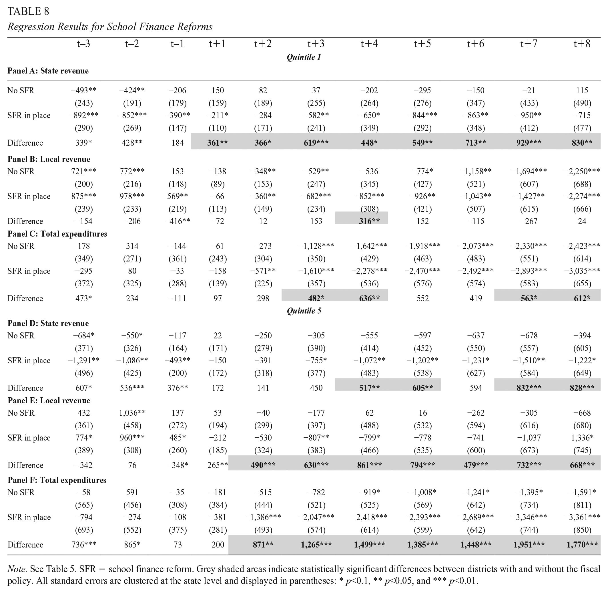
Note. See Table 5. SFR = school finance reform. Grey shaded areas indicate statistically significant differences between districts with and without the fiscal policy. All standard errors are clustered at the state level and displayed in parentheses: * p<0.1, ** p<0.05, and *** p<0.01.

Table 5 presents recession effects for districts with and without strict BBRs. Low-income districts with strict BBRs experienced less growth in state aid than did districts without strict BBRs. Gaps were statistically different from zero after the second post year and ranged between $708–$1,355 per pupil. The revenue differences were reflected in large spending disparities between both groups of districts, but these differences were not statistically significant.

Table 6 reveals few statistically significant differences between districts with and without state TELs. Because these differences were not corroborated by our falsification and robustness checks, presented in the appendices, they are not discussed further. Local TELs, on the other hand, had a profound impact on district budgets, as shown in Table 7. State aid increased less in low-income districts with local TELs than in low-income districts without local TELs. The statistically significant gaps varied between $760–$1,440 per pupil. Total expenditures reflected these impacts (see Panel C of Table 7). Quintile 5 districts were also affected by local TELs, but the underlying mechanism differed from that of Quintile 1 districts. High-income districts with local TELs were unable to increase local revenues at the same rate as were high-income districts without local TELs. Disparities grew from $292 in post year 1 to $1,200 in post year 8. Revenue differences were, however, not mirrored for total expenditures in high-income districts.

The differential effect of SFRs on recession impacts is presented in Table 8. For low-income districts, growth in state aid was much less for districts with SFRs than for districts without SFRs. The greatest gap occurred 7 years after the start of the recession, with $929 per pupil. Again, these discrepancies were reflected in total expenditures. High-income districts experienced similar disparities between SFR and non-SFR districts.¹⁷

Endogeneity and Robustness Checks

We performed several endogeneity and robustness checks, which are explained in more detail in Appendices D and E, respectively. The endogeneity checks were based on the work of Brunner et al. (2020). We further added specifications that excluded control variables and estimated additional pre-recession event dummies. Robustness checks included (a) changes in our recession definition based on the fiscal years exposed to a recession, (b) a county-level recession definition, (c) alternative definitions of fiscal institutions and policies, and (d) regression models weighted by student enrollment. All falsification and robustness checks corroborated our initial findings or had the expected results.

Discussion and Conclusion

This study investigated two research questions: (a) How did the Great Recession affect revenues and expenditures in low- and high-income school districts? and (b) How did fiscal institutions and policies shape the impact of the Great Recession on low- and high-income school district finances? Regarding the first question, we find greater recession effects on school district total revenues and expenditures than earlier studies have (Chakrabarti et al., 2014, 2015; Evans et al., 2019; Leachman, 2019; Oliff & Leachman, 2011). The findings are comparable, however, with recent scholarship (Jackson et al., 2021).

Our conclusions for state and local revenues challenge earlier findings in the literature. We have provided evidence that not only low-income districts (Evans et al., 2019; Jackson et al., 2021), but also high-income districts experienced declines in state aid. This finding was potentially driven by SFR, as we discuss below. The result for local revenue challenges previous arguments emphasizing the stability of the property tax and the potential use of local taxes to offset reductions in state aid (Evans et al., 2019). Our findings are comparable to those of studies emphasizing differences between low- and high-income districts in their capacity to offset reductions in state transfers using property taxes (Chakrabarti et al., 2014, 2015).

Concerning the second research question, our hypothesis 1 formulated that low-income districts with strict BBRs experienced greater recession effects than did districts without strict BBRs. Our findings corroborate this claim and stress the importance of intergovernmental relations for financing K–12 education in the United States (Wirt & Kirst, 2001). More specifically, we have provided evidence that state fiscal institutions influenced budgets of local governments that were dependent on their transfers. To the best of our knowledge, we are the first to empirically describe this relationship in the context of K–12 education.

State TELs did not, as claimed in hypothesis 2, influence school district finances. Local TELs, conversely, reduced the growth in local revenues for high-income districts. Our findings suggest that strategies to overcome the constraining effects of local TELs described in the literature, such as increases in state aid, overrides, and growth in non–property tax revenues (Downes & Figlio, 2015), were not effective during the Great Recession. We suspect that these strategies were affected by the economic decline as well, because states needed to cut budgets, while local voters were unwilling or unable to increase school district resources. We are the first, to our knowledge, to present this evidence.

We find, furthermore, an effect of local TELs on state aid for low-income districts that has not been discussed in the literature. Although an in-depth analysis of this effect is beyond the scope of this study, we can bring forward potential explanations for its occurrence. First, several studies have argued that local revenue shortfalls, imposed by TELs, were offset by increases in state aid to school districts (Downes & Figlio, 2015).¹⁸ States could have reduced these transfers, which were neither mandated nor court-ordered, under fiscal stress. Second, we note that strict BBRs and local TELs were correlated by a factor of 0.5. The impact of local TELs on state aid for low-income school districts could have been, therefore, spurious and driven by strict BBRs. The impact of local TELs on state aid, however, was still sizable but less precise when we used an alternative measure of local TELs in our robustness checks that was less correlated with strict BBRs (0.3). This result potentially indicates that the relationship between local TELs and state aid in low-income districts was independent of BBRs and more complex than discussed in the literature.

Finally, our last hypothesis asserted that low-income districts with SFRs experienced greater recession effects than did districts without them. The centralization of revenue sources, introduced by SFRs, made school districts more dependent on elastic tax sources and state-level decision-makers who were not directly influenced by reductions in transfers to school districts. As a result, state aid to local school districts declined during the recession, as also found by Jackson et al. (2021).

We also identified a relationship between state aid and SFRs in high-income school districts during recessions that has not been covered in earlier studies. Once more, we cannot explore this relationship in depth, but we can provide potential explanations. For instance, high-income districts received state transfers, even though these transfers were less than those for low-income districts (see Table 3). During recessions, states could have decreased these transfers to reduce cutbacks in other spending categories. Furthermore, states might have reduced matching rates for grants, decreasing incentives to apply for them. As a consequence, spending for capital projects or specialty programs, such as improving teaching quality; science, technology, engineering, and math education; or career education, could have been reduced.

Future studies could build upon the unanswered questions raised. Specifically, we have provided evidence of reductions in state aid during a recession for low-income districts with local TELs. Future research could discuss and explain the mechanisms behind this phenomenon. Additionally, high-income districts received less state aid if they were exposed to SFRs, even though these districts did not benefit from equity reforms. Once again, additional studies could explore the mechanism behind this curious finding. Another shortcoming of our analysis is that fiscal institutions and policies were measured prior to the Great Recession. Although minimal change occurred, future scholarly work could explore whether economic downturns affect revising fiscal institution laws and policies. One robustness check revealed that the main results were sensitive to weighting by enrollment. To our knowledge, no literature addresses a relationship between district size and recession effects or fiscal policies that could explain these findings. We conceptualized that high-income districts might vary in tax bases across enrollments, which generated differential reductions in local revenue post-recession. Because operating costs were greatest for small districts that lacked economies of scale (Duncombe & Yinger, 2007, 2008), we conceptualized that differences in managerial decision-making about recession spending cuts for the smallest districts may have driven differential total expenditure results. Moreover, fiscal institutions might have constrained tax bases and managerial decisions differently by size of the district. These expectations create another area for future exploration. Lastly, we find greater cuts in total per-pupil expenditures than revenues. Future research could address this question and evaluate what drives the gap between reductions in school districts’ revenue and spending.

Supplemental Material

sj-docx-1-ero-10.1177_23328584231189176 – Supplemental material for The Interplay Between Fiscal Institutions and the Great Recession: Evidence From U.S. School Districts

Supplemental material, sj-docx-1-ero-10.1177_23328584231189176 for The Interplay Between Fiscal Institutions and the Great Recession: Evidence From U.S. School Districts by Christian Buerger and Michelle L. Lofton in AERA Open

Footnotes

ORCID iDs

Christian Buerger

Michelle L. Lofton

Supplemental Material

Supplemental material for this article is available online.

Notes

Authors

CHRISTIAN BUERGER is an assistant professor at Indiana University in Indianapolis. His research focuses on topics in program evaluation, public management, education policy, and public finance.

MICHELLE L. LOFTON is an assistant professor in the Department of Public Administration and Policy at the University of Georgia; email: mlofton@uga.edu. Her core research investigates financial tools used for public cash flow management and the impacts of fiscal institutions on government finances, especially during recessions and periods of high financial uncertainty.

References

Aastveit

K. A.

Jore

A. S.

Ravazzolo

(2016). Identification and real-time forecasting of Norwegian business cycles. International Journal of Forecasting, 32(2), 283–292.

Abrams

B. A.

Dougan

W. R.

(1986). The effects of constitutional restraints on governmental spending. Public Choice, 49(2), 101–116.

Afonso

W. B.

(2013). Coping with the Great Recession: Theory and practice for county governments. International Journal of Public Administration, 36(11), 768–779.

Alt

J. E.

Lowry

R. C.

(1994). Divided government, fiscal institutions, and budget deficits: Evidence from the states. American Political Science Review, 88(4), 811–828.

Amiel

Deller

S. C.

Stallmann

J. I.

(2009). The construction of a tax and expenditure limitation index for the U.S. University of Wisconsin-Madison Department of Agricultural & Applied Economics. Staff Paper Series. Staff Paper No. 536. https://ageconsearch.umn.edu/record/92231/?ln=en

Amiel

Deller

Stallmann

Maher

(2014). Does the restrictiveness of state tax and expenditure limitations affect state revenues and expenditures? International Journal of Public Administration, 37(4), 237–248.

Anglum

J. C.

Shores

K. A.

Steinberg

M. P.

(2021). Federal stimulus aid and school finance: Lessons from the Great Recession (EdWorkingPaper No. 21-497). Annenberg Institute for School Reform at Brown University.

Angrist

J. D.

Pischke

(2008). Mostly harmless econometrics: An empiricist’s companion. Princeton University Press

Autor

D. H.

(2003). Outsourcing at will: The contribution of unjust dismissal doctrine to the growth of employment outsourcing. Journal of Labor Economics, 21(1), 1–42.

10.

Bails

D. G.

(1982). A critique on the effectiveness of tax-expenditure limitations. Public Choice, 38(2), 129–138.

11.

Bails

D. G.

(1990). The effectiveness of tax-expenditure limitations: A re-evaluation: In 19 states they resulted in virtually no success in limiting growth in their budgets. American Journal of Economics and Sociology, 49(2), 223–238.

12.

Baker

B. D.

(2014). Evaluating the recession’s impact on state school finance systems. Education Policy Analysis Archives/Archivos Analíticos de Políticas Educativas, 22, 1–30.

13.

Barnum

(2020, April 22). 12 ways the last recession changed America’s schools—and what that means for the years ahead. Chalkbeat. https://www.chalkbeat.org/2020/4/22/21230992/great-recession-schools-research-lessons-coronavirus

14.

Berge

T. J.

Jordà

(2013). A chronology of turning points in economic activity: Spain, 1850–2011. SERIEs, 4(1), 1–34.

15.

Bohn

Inman

R. P.

(1996). Balanced-budget rules and public deficits: Evidence from the U.S. states. Carnegie-Rochester Conference Series on Public Policy, 45, 13–76.

16.

Bourdeaux

Warner

(2015). School districts’ expenditure responses to federal stimulus funds. Journal of Education Finance, 41(1), 30–47.

17.

Bruce

Fox

W. F.

Tuttle

M. H.

(2006). Tax base elasticities: A multi-state analysis of long-run and short-run dynamics. Southern Economic Journal, 73(2), 315–341.

18.

Brunner

Hyman

(2020). School finance reforms, teachers’ unions, and the allocation of school resources. Review of Economics and Statistics, 102(3), 473–489.

19.

Bry

Boschan

(1971). Programmed selections of cyclical turning points. In Gerhard

Boschan

(Eds.), Cyclical analysis of time series: Selected procedures and computer programs (pp. 7–63). National Bureau of Economic Research.

20.

Buerger

(2021). The effect of economic downturns on state budgets: A counterfactual analysis of the Great Recession. Applied Economics Letters, 28(21), 1852–1859.

21.

Buerger

Sandel

R. M.

Reitano

Lofton

M. L.

Jones

(2021). Extending differences-in-differences frameworks to Granger equations: Evidence from cutback management during three recessions. International Journal of Public Sector Management, 34(6), 688–705.

22.

Card

Krueger

(1994). Minimum wages and employment: A case study of the fast-food industry in New Jersey and Pennsylvania. American Economic Review, 84(4), 772–793.

23.

Cameron

A. C.

Trivedi

P. K.

(2005). Microeconometrics: Methods and applications. Cambridge University Press.

24.

Chakrabarti

Livingston

Roy

(2014). Did cuts in state aid during the Great Recession lead to changes in local property taxes? Education Finance and Policy, 9(4), 383–416.

25.

Chakrabarti

Livingston

Setren

(2015). The Great Recession’s impact on school district finances in New York State. Federal Reserve Bank of New York Economic Policy Review, 12(1), 45–66.

26.

Chernick

Langley

Reschovsky

(2011). The impact of the Great Recession and the housing crisis on the financing of America’s largest cities. Regional Science and Urban Economics, 41(4), 372–381.

27.

Colombo

Lazzari

(2020). Same, but different? A state-level chronology of the 2014–2016 Brazilian economic recession and comparisons with the GFC and (early data on) COVID-19. Economics Bulletin, 40(3).

28.

Corcoran

S. P.

Evans

W. N.

(2015). Equity, adequacy, and the evolving state role in education finance. In Ladd

H. F.

Goertz

M. E.

(Eds.), Handbook of research in education finance and policy (2nd ed., pp. 353–375). Routledge.

29.

Costello

A. M.

Petacchi

Weber

J. P.

(2017). The impact of balanced budget restrictions on states’ fiscal actions. Accounting Review, 92(1), 51–71.

30.

Cox

Lowery

(1990). The impact of the tax revolt era state fiscal caps. Social Science Quarterly, 71(3), 492–509.

31.

Crain

W. M.

(2003). Volatile states: Institutions, policy, and the performance of American state economies. University of Michigan Press.

32.

Crone

T. M.

(2006). What a new set of indexes tells us about state and national business cycles. Federal Reserve Bank of Philadelphia.

33.

Crone

T. M.

Clayton-Matthews

(2005). Consistent economic indexes for the 50 states. Review of Economics and Statistics, 87(4), 593–603.

34.

Deller

Maher

Stallmann

(2021). Do tax and expenditure limitations exacerbate rising income inequality? Economics and Politics, 33(3), 611–643. https://doi.org/10.1111/ecpo.12177

35.

Domina

Pharris-Ciurej

Penner

A. M.

Penner

E. K.

Brummet

Porter

S. R.

Sanabria

(2018). Is free and reduced-price lunch a valid measure of educational disadvantage? Educational Researcher, 47(9), 539–555.

36.

Downes

T. A.

Figlio

D. N.

(2015). Tax and expenditure limits, school finance, and school quality. In Ladd

H. F.

Goertz

M. E.

(Eds.), Handbook of research in education finance and policy (2nd ed., pp. 392–407). Routledge.

37.

Downes

Killeen

K. M.

(2014). So slow to change: The limited growth of nontax revenues in public education finance, 1991–2010. Education Finance and Policy, 9(4), 567–599.

38.

Driscoll

J. C.

Kraay

A. C.

(1998). Consistent covariance matrix estimation with spatially dependent panel data. Review of Economics and Statistics, 80(4), 549–560.

39.

Duncombe

Yinger

(2007). Does school district consolidation cut costs? Education Finance and Policy, 2(4), 341–375.

40.

Duncombe

Yinger

(2008). Measurement of cost differentials. In Ladd

H. F.

Fiske

E. B.

(Eds.), Handbook of research in education finance and policy (1st ed., pp. 238–256). Routledge.

41.

Dye

R. F.

McGuire

T. J.

(1997). The effect of property tax limitation measures on local government fiscal behavior. Journal of Public Economics, 66(3), 469–487. https://doi.org/10.1016/S0047-2727(97)00047-9

42.

Dye

R. F.

McGuire

T. J.

McMillen

D. P.

(2005). Are property tax limitations more binding over time? National Tax Journal, 58(2), 215–225.

43.

Eom

T. H.

Duncombe

Nguyen-Hoang

Yinger

(2014). The unintended consequences of property tax relief: New York’s STAR program. Education Finance and Policy, 9(4), 446–480.

44.

Evans

W. N.

Schwab

R. M.

Wagner

K. L.

(2019). The Great Recession and public education. Education Finance and Policy, 14(2), 298–326.

45.

Goldstein

McGee

J. B.

(2021). Did spending cuts during the Great Recession really cause student outcomes to decline? Education Reform Faculty and Graduate Students Publications.

46.

Gordon

(2004). Do federal grants boost school spending? Evidence from Title I. Journal of Public Economics, 88(9–10), 1771–1792.

47.

Gordon

T. M.

(2008). The calculus of constraint: A critical review of state fiscal institutions. In Garrett

Graddy

E. A.

Jackson

H. E.

(Eds.), Fiscal challenges: An interdisciplinary approach to budget policy (pp. 217–289). Cambridge University Press.

48.

Gordon

T. M.

(2012). State and local fiscal institutions in recession and recovery. In Ebel

R. D.

Petersen

J. E.

(Eds.), The Oxford handbook of state and local government finance (pp. 246–267). Oxford University Press.

49.

Granger

C. W. J.

(1969). Investigating causal relations by econometric models and cross-spectral methods. Econometrica, 37(3), 424–438.

50.

Greene

(2003). Econometrics (5th ed.). Pearson

51.

Groves

H. M.

Kahn

C. H.

(1952). The stability of state and local tax yields. American Economic Review, 42(1), 87–102.

52.

Gruber

(2005). Public finance and public policy. Macmillan.

53.

Hainmueller

Mummolo

(2019). How much should we trust estimates from multiplicative interaction models? Simple tools to improve empirical practice. Political Analysis, 27(2), 163–192.

54.

Hamilton

J. D.

Owyang

M. T.

(2012), The propagation of regional recessions. Review of Economics and Statistics, 94(4), 935–947.

55.

Harding

Pagan

(2003). A comparison of two business cycle dating methods. Journal of Economic Dynamics and Control, 27(9), 1681–1690.

56.

Hendrick

R. M.

Garand

J. C.

(1991). Expenditure tradeoffs in the US states: A pooled analysis. Journal of Public Administration Research and Theory, 1(3), 295–318.

57.

Hill

A. J.

Jones

D. B.

(2017). Does partisan affiliation impact the distribution of spending? Evidence from state governments’ expenditures on education. Journal of Economic Behavior and Organization, 143, 58–77.

58.

Hines

J. R.

Jr. Thaler

R. H.

(1995). Anomalies: The flypaper effect. Journal of Economic Perspectives, 9(4), 217–226.

59.

Holcombe

R. G.

Sobel

R. S.

(1995). The relative variability of state income and sales taxes over the revenue cycle. Atlantic Economic Journal, 23(2), 97–112.

60.

Hong

(2015). Fiscal rules in recessions: Evidence from the American states. Public Finance Review, 43(4), 505–528.

61.

Hou

(2001). Testing the effects of sub-national counter-cyclical fiscal policies: Budget stabilization funds, general fund surpluses, and state total own-source expenditures. Syracuse University.

62.

Hou

(2013). State government budget stabilization: Policy, tools, and impacts (Vol. 8). Springer.

63.

Hou

Smith

D. L.

(2006). A framework for understanding state balanced budget requirement systems: Reexamining distinctive features and an operational definition. Public Budgeting and Finance, 26(3), 22–45.

64.

Hou

Smith

(2010). Do state balanced budget requirements matter? Testing two explanatory frameworks. Public Choice, 145(1–2), 57–79.

65.

Howard

M. A.

(1989). State tax and expenditure limitations: There is no story. Public Budgeting and Finance, 9(2), 83–90.

66.

Jackson

C. K.

Johnson

Persico

(2014). The effect of school finance reforms on the distribution of spending, academic achievement, and adult outcomes (NBER Working Paper No. 20118). National Bureau of Economic Research. https://www.nber.org/papers/w20118

67.

Jackson

C. K.

Wigger

Xiong

(2021). Do school spending cuts matter? Evidence from the Great Recession. American Economic Journal: Economic Policy, 13(2), 304–335.

68.

Jimenez

B. S.

(2017). Institutional constraints, rule-following, and circumvention: Tax and expenditure limits and the choice of fiscal tools during a budget crisis. Public Budgeting and Finance, 37(2), 5–34.

69.

Joyce

P. G.

Mullins

D. R.

(1991). The changing fiscal structure of the state and local public sector: The impact of tax and expenditure limitations. Public Administration Review, 51(3), 240–253.

70.

Kenyon

D. A.

Benker

K. M.

(1984). Fiscal discipline: Lessons from the state experience. National Tax Journal, 37(3), 433–446.

71.

Kim

(2017). Limits of property taxes and charges: City revenue structure after the Great Recession. Urban Affairs Review, 55(1), 185–209. https://doi.org/10.1177/1078087417697199

72.

Kim

Warner

M. E.

(2018). Shrinking local autonomy: Corporate coalitions and the subnational state. Cambridge Journal of Regions, Economy and Society, 11(3), 427–441.

73.

King

R. G.

Plosser

C. I.

(1994). Real business cycles and the test of the Adelmans. Journal of Monetary Economics, 33(2), 405–438.

74.

Kioko

S. N.

Lofton

M. L.

(2021). Balanced budget requirements revisited. Public Finance Review, 49(5), 635–672.

75.

Knight

D. S.

(2017). Are high-poverty school districts disproportionately impacted by state funding cuts? School finance equity following the Great Recession. Journal of Education Finance, 43(2), 169–194.

76.

Kousser

McCubbins

M. D.

Moule

(2008). For whom the TEL tolls: Can state tax and expenditure limits effectively reduce spending? State Politics and Policy Quarterly, 8(4), 331–361.

77.

Lafortune

Rothstein

Schanzenbach

D. W.

(2018). School finance reform and the distribution of student achievement. American Economic Journal: Applied Economics, 10(2), 1–26.

78.

Langley

A. H.

(2016). Local government finances during and after the Great Recession. In McCarthy

G. W.

Ingram

G. K.

Moody

S. A.

(Eds.), Land and City (pp. 171–196). Lincoln Institute of Land Policy.

79.

Layton

A. P.

Banerji

(2003). What is a recession? A reprise. Applied Economics, 35(16), 1789–1797.

80.

Leachman

(2019, May 29). K–12 funding still lagging in many states. Center on Budget and Policy Priorities. https://www.cbpp.org/blog/k-12-funding-still-lagging-in-many-states

81.

Leachman

Masterson

Figueroa

(2017, November 29). A punishing decade for school funding. Center on Budget and Policy Priorities. https://www.cbpp.org/research/state-budget-and-tax/a-punishing-decade-for-school-funding

82.

Lowery

(1983). Limitations on taxing and spending powers: An assessment of their effectiveness. Social Science Quarterly, 64(2), 247.

83.

Lukemeyer

(2003). Courts as policymakers: School finance reform litigation. LFB Scholarly Publishing LLC.

84.

Lutz

B. F.

(2008). The connection between house price appreciation and property tax revenues. National Tax Journal, 61(3), 555–572.

85.

Lyons

Lav

I. J.

(2007). The problems with property tax revenue caps. Center on Budget and Policy Priorities. https://www.cbpp.org/sites/default/files/archive/6-21-07sfp.pdf

86.

Mahdavi

Westerlund

(2011). Fiscal stringency and fiscal sustainability: Panel evidence from the American state and local governments. Journal of Policy Modeling, 33(6), 953–969.

87.

Maher

C. S.

Park

Harrold

(2016). The effects of tax and expenditure limits on municipal pension and OPEB funding during the Great Recession. Public Finance and Management, 16(2).

88.

McCubbins

M. D.

Moule

(2010). Making mountains of debt out of molehills: The pro-cyclical implications of tax and expenditure limitations. National Tax Journal, 63(3), 603–621.

89.

McGuire

T. J.

(1999). Proposition 13 and its offspring: For good or for evil? National Tax Journal, 52(1), 129–138.

90.

Meyer

B. D.

(1995), Natural and quasi-experiments in economics. Journal of Business Economics and Statistics, 13(2), 151–161.

91.

Mullins

D. R.

(2004). Tax and expenditure limitations and the fiscal response of local government: Asymmetric intra-local fiscal effects. Public Budgeting and Finance, 24(4), 111–147.

92.

Mullins

D. R.

Joyce

P. G.

(1996). Tax and expenditure limitations and state and local fiscal structure: An empirical assessment. Public Budgeting and Finance, 16(1), 75–101. https://doi.org/10.1111/1540-5850.01061

93.

Mullins

D. R.

Wallin

B. A.

(2004). Tax and expenditure limitations: Introduction and overview. Public Budgeting and Finance, 24(4), 2–15.

94.

Musso

J. A.

Graddy

E. A.

Grizard

J. B.

(2008). Budgetary arrangements in the 50 states. In Jackson

H. E.

Graddy

E. A.

Garrett

(Eds.), Fiscal challenges: An interdisciplinary approach to budget policy (pp. 251–270). Cambridge University Press.

95.

National Bureau of Economic Research (NBER). (2023). Business Cycle Dating. https://www.nber.org/research/business-cycle-dating#:~:text=The%20NBER’s%20definition%20emphasizes%20that,more%20than%20a%20few%20months

96.

Oliff

Leachman

(2011, October 7). New school year brings steep cuts in state funding for schools. Center on Budget and Policy Priorities. https://www.cbpp.org/research/new-school-year-brings-steep-cuts-in-state-funding-for-schools

97.

O’Toole

Stipak

(2000). Oregon school districts respond to increased tax limitations. Journal of Education Finance, 26(2), 173–186.

98.

Owyang

M. T.

Piger

Wall

H. J.

(2005). Business cycle phases in US states. Review of Economics and Statistics, 87(4), 604–616.

99.

Pagano

Hoene

C. W.

(2018). City budgets in an era of increased uncertainty. Metropolitan Policy Program at Brookings. https://www.brookings.edu/wp-content/uploads/2018/07/20180718_Brookings-Metro_City-fiscal-policy-ES-Pagano-Hoene.pdf

100.

Park

J. H.

Park

Maher

C. S.

(2018). The effects of tax and expenditure limitations (TELs) on municipal fiscal outcomes during a period of fiscal distress. Public Finance and Management, 18(1), 84–110.

101.

Poterba

J. M.

(1994). State responses to fiscal crises: The effects of budgetary institutions and politics. Journal of Political Economy, 102(4), 799–821.

102.

Raudla

Savi

Randma-Liiv

(2013). Literature review on cutback management. RePub. https://repub.eur.nl/pub/40927/

103.

Rose

(2006). Do fiscal rules dampen the political business cycle? Public Choice, 128(3–4), 407–431.

104.

Rose

(2010). Institutions and fiscal sustainability. National Tax Journal, 63(4), 807–838.

105.

Rothbart

M. W.

(2020). Does school finance reform reduce the race gap in school funding? Education Finance and Policy, 15(4), 675–707.

106.

Rueben

Randall

Boddupalli

(2018). Budget processes and the Great Recession: How state fiscal institutions shape tax and spending decisions. Proceedings. Annual Conference on Taxation and Minutes of the Annual Meeting of the National Tax Association, 111, i–viii, 1–60. https://www.jstor.org/stable/26939526

107.

Sexton

T. E.

Sexton

R. J.

(1986). Re-evaluating the income elasticity of the property tax base. Land Economics, 62(2), 182–191.

108.

Shadbegian

R. J.

(1996). Do tax and expenditure limitations affect the size and growth of state government? Contemporary Economic Policy, 14(1), 22–35.

109.

Shadbegian

R. J.

(1998). Do tax and expenditure limitations affect local government budgets? Evidence from panel data. Public Finance Review, 26(2), 118–136.

110.

Shadbegian

R. J.

(1999). The effect of tax and expenditure limitations on the revenue structure of local government, 1962–87. National Tax Journal, 52(2), 221–237.

111.

Shores

Steinberg

M. P.

(2019a). The Great Recession, fiscal federalism and the consequences for cross-district spending inequality. Journal of Education Finance, 45(2), 123–148.

112.

Shores

Steinberg

M. P.

(2019b). Schooling during the Great Recession: Patterns of school spending and student achievement using population data. AERA Open, 5(3), 1–29.

113.

Shores

Steinberg

M. P.

(2022). Fiscal federalism and K–12 education funding: Policy lessons from two educational crises. Educational Researcher, 51(8), 551–558.

114.

Skidmore

Tosun

M. S.

(2011). Property value assessment growth limits, tax base erosion, and regional in-migration. Public Finance Review, 39(2), 256–287.

115.

Sobel

R. S.

Holcombe

R. G.

(1996). Measuring the growth and variability of tax bases over the business cycle. National Tax Journal, 49(4), 535–552.

116.

Stallmann

J. I.

Maher

C. S.

Deller

S. C.

Park

(2017). Surveying the effects of limitations on taxes and expenditures: What do/don’t we know? Journal of Public and Nonprofit Affairs, 3(2), 197–222.

117.

Stock

J. H.

Watson

M. W.

(1989). New indexes of coincident and leading economic indicators. NBER Macroeconomics Annual, 4, 351–394.

118.

Strunk

K. O.

Marianno

B. D.

(2019). Negotiating the Great Recession: How teacher collective bargaining outcomes change in times of financial duress. AERA Open, 5(2), 1–18.

119.

Sun

(2014). Reevaluating the effect of tax and expenditure limitations: An instrumental variable approach. Public Finance Review, 42(1), 92–116.

120.

Swain

W. A.

Redding

(2019). Teachers’ union power in a budget crunch: Lasting ramifications of differential spending responses to the great recession. Educational Policy, 36(2), 343–376.

121.

Tsai

P.-H.

(2014). State fiscal rules and composition changes in public spending before the election. Public Finance Review, 42(1), 58–91.

122.

Wagner

G. A.

(2003). Are state budget stabilization funds only the illusion of savings? Evidence from stationary panel data. Quarterly Review of Economics and Finance, 43(2), 213–238.

123.

Wagner

G. A.

Elder

(2007). Revenue cycles and the distribution of shortfalls in U.S. states: Implications for an “optimal” rainy day fund. National Tax Journal, 60(4), 727–742.

124.

Wen

Kim

Warner

M. E.

(2020). Starving counties, squeezing cities: Tax and expenditure limits in the US. Journal of Economic Policy Reform, 23(2), 101–119.

125.

Wirt

Kirst

(2001). The political dynamics of American education (2nd ed.). McCutchan.

126.

Wooldridge

J. M.

(2009). Introductory econometrics: A modern approach. Thomson.

127.

Yagan

(2019). Employment hysteresis from the Great Recession. Journal of Political Economy, 127(5), 2505–2558.

128.

Yang

(2017). Financial management conservatism under constraints: Tax and expenditure limits and local deficit financing during the Great Recession. Local Government Studies, 43(6), 946–965.

129.

Yinger

(Ed.). (2004). State aid and the pursuit of educational equity: An overview. In Helping children left behind: State aid and the pursuit of educational equity (pp. 3–58). MIT Press.

Supplementary Material

Please find the following supplemental material available below.

For Open Access articles published under a Creative Commons License, all supplemental material carries the same license as the article it is associated with.

For non-Open Access articles published, all supplemental material carries a non-exclusive license, and permission requests for re-use of supplemental material or any part of supplemental material shall be sent directly to the copyright owner as specified in the copyright notice associated with the article.

0.00 MB

0.42 MB