Sage Journals: Discover world-class research

Abstract

Loudness is a fundamental dimension of auditory perception. When hearing impairment results in a loudness deficit, hearing aids are typically prescribed to compensate for this. However, the relationship between an individual’s specific hearing impairment and the hearing aid fitting strategy used to address it is usually not straightforward. Various iterations of fine-tuning and troubleshooting by the hearing care professional are required, based largely on experience and the introspective feedback from the hearing aid user. We present the development of a new method for validating an individual’s loudness perception of natural signals relative to a normal-hearing reference. It is a measurement method specifically designed for the situation typically encountered by hearing care professionals, namely, with hearing-impaired individuals in the free field with their hearing aids in place. In combination with the qualitative user feedback that the measurement is fast and that its results are intuitively displayed and easily interpretable, the method fills a gap between existing tools and is well suited to provide concrete guidance and orientation to the hearing care professional in the process of individual gain adjustment.

Keywords

hearing loss perceptual evaluation amplification gain dynamic range compression

Introduction

The psychophysical dimension of loudness is an important component of auditory perception. People affected by hearing impairment typically associate it with a deficit in loudness perception. Various primarily audiogram-based hearing aid fitting methods exist, for example, NAL-NL2 (Keidser et al., 2011, 2012), DSL v5.0 (Scollie et al., 2005), CAM2 (Moore et al., 2010), or the proprietary fitting methods of the large hearing aid manufacturers. The differences in gains prescribed by various fitting methods for the same audiogram can be substantial, sometimes reaching values up to 20 dB (Dillon, 2012). For individuals with similar audiograms, the gains required to compensate for an altered loudness perception can also vary significantly (Oetting et al., 2018).

Depending on the fitting method, assessment of a hearing-impaired individual’s loudness perception and its relationship with “normal” loudness perception has historically played a role at different stages of the process of hearing aid fitting. On the one hand, the fitting strategy itself may be based on the idea of normalizing loudness perception; examples include the LGOB (Allen et al., 1990), FIG6 (Killion & Fikret-Pasa, 1993), DSL[i/o] (Cornelisse et al., 1995), ScalAdapt (Kiessling et al., 1996), RAB (Ricketts, 1996), IHAFF (Valente & Van Vliet, 1997), and CAMREST (Moore, 2000) fitting procedures and protocols. On the other hand, loudness assessments may be used to verify or validate an existing fit: The APHAB questionnaire (Cox & Alexander, 1995), for instance, is an integral part of the IHAFF fitting protocol. Cox and Gray (2001) argued in favor of routinely conducting aided free-field loudness measurements in validating the results of a hearing aid fit, while Aazh and Moore (2007) stressed the importance of aided real-ear insertion gain (REIG) measurements in verifying the performance of a hearing aid after the fit. Finally, while Oetting et al. (2018) illustrated how aided loudness measurements can be helpful in validating the outcome of a fitting procedure, Kramer et al. (2020) used such measurements to compare different fitting strategies. Thus, depending on context, loudness assessment (in the broadest sense) in the fitting of hearing aids has taken many different forms: from self-assessment inventories like APHAB (Cox & Alexander, 1995) to audiogram-based loudness predictions like in DSL[i/o] (Cornelisse et al., 1995) or CAMREST (Moore, 2000), physical real-ear verification measurements (Aazh & Moore, 2007), and unaided or aided psychoacoustic validation measurements. It is such aided, free-field, binaural, suprathreshold loudness perception measurements (Dermody & Byrne, 1975, being an early example of such measurements) that the current article will focus on.

To assess the degree to which the individual gains compensate for a given individual’s hearing deficit in terms of loudness, it is necessary to test the loudness perception of the hearing aid users after the first fit of their devices. One of the most widely used loudness measurement procedures at present is probably the categorical loudness scaling method (CLS). Several versions have been proposed, for example, LGOB (Allen et al., 1990), Contour (Cox et al., 1997), NAL-ACLS (Keidser et al., 1999), or ACALOS (Brand & Hohmann, 2002); the method is also standardized (International Organization for Standardization [ISO], 2006). While theoretically well-founded and long-established, we argue that CLS has certain drawbacks that come into play when applying the method to aided free-field measurements with hearing aids, that is, precisely the scenario that the method described in this article (the Loudness Validation Method, or LVM), sets out to address. Typically, the signals used in the CLS approach have rather steep onset slopes of 50 ms. This does not always give the dynamic range compression algorithms in the hearing aids sufficient time to reach a steady state, which can lead to overshoots (Souza, 2002). Under the assumption that the perceived overall loudness of a time-varying signal corresponds, by and large, to the loudness of its loudest portion (defined as N₅, i.e., the “loudness which is reached or exceeded in 5% of the measurement time”; Fastl & Zwicker, 2007, p. 323), such overshoots can result in a bias in the loudness judgments of aided test subjects. Furthermore, the noise signals used as stimuli could be recognized as (unwanted) background noise by some hearing aids, thus triggering automatic noise reduction algorithms and, again, distorting the test results in a way that is difficult to control or even identify. By using natural signals, the LVM circumvents this problem for most of the stimuli. On the practical side, the interpretation of exactly which gain function in the hearing aid fitting software (e.g., G₅₀, G₆₅, or G₈₀) needs to be corrected in what way given the (narrowband) CLS loudness function is not straightforward. Finally, the values of the loudness functions found by the CLS algorithm at very low levels can be influenced by hearing aid system noise. This can influence the overall shape of the curve, potentially also leading to biased interpretations of the results.

Like the method presented in this article, Smeds et al. (2006a, 2006b) used free-field natural signals to validate loudness perception in the laboratory (where signals were presented in stereo via two loudspeakers located at a distance of 1.8 m in front of the subjects, on each side of a television screen) as well as in the field, for both normal-hearing and aided hearing-impaired subjects, all of which were (among other conditions) fitted with research hearing aids. The subjects were presented with 11 speech and non-speech audiovisual signals with a duration between 13 and 21 s and a level between 46 and 86 dB(C) SPL, with the presentation levels in the laboratory corresponding to the actual levels of the corresponding recorded events in the field. Differing in its goals from the method described here, one of the objectives of the studies was to assess the preferred overall loudness of the subjects relative to the predictions of a loudness model (Moore & Glasberg, 1997). Among their findings was the fact that the preferred overall loudness of normal-hearing subjects and, to an even greater extent, hearing-impaired subjects differed significantly, depending on whether the listening situation was in the laboratory or in the field. At first glance, this seems to be posing a problem for any approach that aims at using subjective loudness ratings from the laboratory to improve the subjects’ loudness perception in real life. However, as explained below, the method described here uses reference values as a standard of comparison which were derived with the same method and under the same conditions from a group of normal-hearing subjects, thereby analyzing the difference in overall loudness perception between normal-hearing and hearing-impaired subjects. Any discrepancies between laboratory and field that remain when the subjects return to their everyday life will then be addressed by the hearing care professional when fine-tuning the hearing aids.

To test the loudness perception of hearing aid users after the first fit, we have developed the LVM, which is specifically designed for the scenario of assessing the loudness perception of aided subjects, that is, of hearing aid users with their fitted devices in place. The method has been developed in-house at the authors’ institution, and various stages of its development have been documented in a series of hitherto mostly informal works (Hoffmann, 2021; Jansen, 2020; Jansen et al., 2020, 2021). The present article provides the first complete and coherent description of the development and evaluation of the method.

To ensure the suitability of the LVM for practical use, a deliberate decision was taken to directly involve hearing care professionals at many stages during the development of the method. The LVM has been used by the audiologists in our in-house hearing aid counseling service since May 2022, and regular feedback rounds were conducted with ∼ 20 independent local hearing care professionals acting as pilot users of the LVM, leading to an optimization of the tool in terms of usability and presentation of the measurement results. In addition, the LVM has been made available as an R&D module for the Oldenburg Measurement Applications (Hörzentrum Oldenburg, 2024) to ∼ 15 selected hearing care professionals at five locations in other parts of Germany in the context of another study. They used the procedure in their daily practice for several months and subsequently gave both direct feedback and feedback via structured interviews and questionnaires, thus contributing to the continuous improvement of the tool.

At the outset, a few notes on the chosen terminology are in order. Firstly, it is argued here that the restoration of normal-hearing loudness perception at the first-fit appointment represents a sensible starting point for the fine-tuning phase, even if other individual factors such as speech intelligibility, listening effort, or sound quality also play a role in hearing aid fitting, which may subsequently lead to deviations from normal loudness perception. Fitting rationales other than loudness normalization, such as loudness equalization (Byrne, 1996) or speech intelligibility maximization (e.g., Keidser et al., 2011, 2012), are not specifically addressed here.

Secondly, the LVM is a method for the validation of the effect of providing a person with a particular hearing aid or fitting strategy with respect to their individual loudness deficit, as opposed to the objective verification of the intervention, for example, by technical real-ear measurements. These are two important, but distinct, concepts, as have been previously discussed in the context of hearing aid provision and public health (e.g., American Speech-Language-Hearing Association [ASHA], 1998; Kochkin, 2011; Palmer et al., 1999).

The basic motivation for the development of the LVM was the realization that, as mentioned above, the restoration of normal loudness perception constitutes a helpful (although not the only possible) starting point for the individual fine-tuning phase of hearing aid fitting (Oetting et al., 2016). Several characteristics of the LVM stand out that, in their combination, make it unique in its practical applicability and distinguish it from other existing methods:

The LVM is designed for the measurement of the loudness perception of hearing-impaired listeners with natural signals. It is therefore ecologically more valid than methods relying purely on artificial noise signals (i.e., making it more relevant for situations that are encountered in real life).

The LVM is a free-field measurement method and is therefore capable of addressing problems with loudness perception that are relevant to challenging everyday situations. This specifically includes binaural loudness perception of broadband signals (Oetting et al., 2016).

The method assesses deviations of an individual’s loudness perception from a normal-hearing reference. In other words, it is used to detect and quantify “non-normal” loudness perception, that is, loudness perception which is either more and less sensitive than the normal-hearing reference. The availability of such a standard of comparison provides hearing care professionals with a helpful reference point for the hearing aid fitting process.

The LVM, by design, is particularly suited for aided measurements (i.e., measurements with hearing devices in place). It can therefore serve as a tool for hearing care professionals to effectively validate whether gain settings in the hearing aids are properly fitted to an individual’s altered loudness perception, and to obtain information as to the exact nature of any problems with the existing fit.

The execution of the LVM measurement procedure is quite fast: Over a total number of 522 measurements conducted at the authors’ institution, the average duration of a complete LVM measurement run was less than six minutes (mean: 05:36 min, standard deviation: 00:44 min). In settings where time is of the essence and measurement durations are an important economic factor, the LVM provides the possibility to achieve practically viable results without compromising accuracy.

Finally, the overall qualitative feedback of the hearing care professionals using the LVM (see above) has been that the results are helpful for the fitting process and that the presentation of the results is intuitive and immediately accessible. Furthermore, the feedback indicates that the LVM result displays are useful in the communication with the customers and that the results are easy to interpret. This focus on user friendliness and ease of applicability is maybe what sets the LVM apart from other existing methods of loudness measurement more than anything else.

Methods

The development of the LVM comprised two parts: First, the stimuli used for the method were developed; then, normal-hearing reference values were determined based on these stimuli. Both steps are described in turn below.

The experiments conducted for the development and evaluation of the method were approved by the responsible ethics committee (“Kommission für Forschungsfolgenabschätzung und Ethik”) of the Carl von Ossietzky University in Oldenburg, Germany (Drs.EK/2019/032 and Drs.EK/2021/031-05, respectively). The test subjects provided their written informed consent and received an allowance for their participation in the experiments.

Development of Stimuli

To control for confounding factors as far as possible, the stimuli used for the LVM were carefully selected and processed in terms of spectral content, presentation level, loudness dynamics, sharpness, shape of empirical response histograms, conspicuous discrepancies between model-based loudness predictions and empirical responses, etc., as detailed below. The LVM procedure was first implemented and developed in MATLAB and subsequently evaluated as an R&D module for the Oldenburg Measurement Applications (Hörzentrum Oldenburg, 2024). Since one of the main design criteria was the use of ecologically valid signals, excerpts from high-quality audio recordings of natural signals from a commercial sound effects library (British Broadcasting Corporation [BBC], 1984) were used as stimuli. The original set of recordings consisted of 667 CD tracks (i.e., WAV files) with a sampling frequency of 44.1 kHz and a resolution of 16 bits. However, to avoid audible quantization noise after overall level adjustment (see below), the resolution of the files was increased to 32 bits.

Next, portions with a duration of either 4 or 5 s were extracted from the tracks. Ramps with a gain rising linearly (on a decibel scale) from −120 to 0 dB (and, correspondingly, falling from 0 to −120 dB) were applied to the beginning and end of each signal, respectively, to avoid unwanted transients that may lead to overshoot from dynamic range compression algorithms. Ramp durations were 1 s at onset and 0.5 s at offset, with the longer ramp duration at the beginning allowing for dynamic range compression algorithms with short or medium attack time constants to settle. It must be born in mind that other hearing aid algorithms which interact with the applied gains (such as signal enhancement algorithms) with longer adaptation time constants may influence the results. It also cannot be ruled out that specific hearing aid models use exceptionally long attack or release times for dynamic range compression that cannot be changed by the hearing care professional.

The following sections describe the way in which the final set of 60 stimuli was derived from that much larger set of original signals. As detailed below, four frequency categories were defined, and the signals were categorized accordingly. Secondly, three presentation level categories were determined empirically, and the signals were scaled to conform to the level category they were assigned to. Finally, several additional criteria were applied both to ensure the general suitability of the signals as LVM stimuli and to choose between different candidate stimuli if more than needed were available.

In order to achieve sufficiently robust results, it was necessary to present several stimuli per category, with the choice of five stimuli found to be a sensible compromise between robustness on the one hand and time efficiency on the other hand: firstly, to address the fairly large spread of responses to be expected in loudness measurements, especially at low levels (Oetting et al., 2014), and secondly, to minimize context effects such as the contrast effect (i.e., the phenomenon that subjects tend to perceive a stimulus as louder if the preceding stimulus is very soft, and vice versa; Arieh & Marks, 2011) or the assimilation effect (i.e., the effect that subjects tend to categorize the loudness of a stimulus similarly to that of a preceding stimulus; Arieh & Marks, 2011).

Definition of Frequency Categories

As mentioned above, for the presentation of the stimuli in the LVM, three level categories (soft, medium, and loud) and four frequency categories (low, middle, high, and broadband) were defined, for a total of 3 × 4 = 12 presentation categories. There were five signals in each category, resulting in a total of 5 × 12 = 60 different stimuli for the entire procedure. To ensure compliance with the respective category specifications as detailed below, the five signals assigned to each category were first scaled in terms of presentation level and then analyzed spectrally. Given the rigorous criteria for the inclusion of a signal as a test stimulus (see below), only a total of 50 out of the 60 signals were unique (six signals were used in two different level categories each, while two signals were used in all three different level categories).

Each of the three narrower frequency categories (henceforth called “narrowband” frequency categories) was psychoacoustically equally wide, spanning six Bark bands each (Fastl & Zwicker, 2007), while the broadband frequency category spanned 3 × 6 = 18 Bark bands, thus approximately covering the frequency range typically transmitted by a hearing aid. The definitions of the frequency ranges for the four LVM frequency bands are given in Table 1.

Table 1.

Definitions of the Frequency Ranges for the Four Loudness Validation Method (LVM) Frequency Categories. See Text for Details.

Frequency category	Frequency range (Bark)	Frequency range (Hz)
Low	Bark bands No. 3–8 (i.e., 2–8 Bark)	200–920
Middle	Bark bands No. 9–14 (i.e., 8–14 Bark)	920–2,320
High	Bark bands No. 15–20 (i.e., 14–20 Bark)	2,320–6,400
Broadband	Bark bands No. 3–20 (i.e., 2–20 Bark)	200–6,400

Finally, all signals were band-pass filtered by a 20th-order type II Chebyshev band-pass filter with cutoff frequencies at 200 and 6,400 Hz to exclude the potential influence of portions of the signals outside the frequency range of hearing aids. While frequencies below 200 Hz may contribute to loudness perception in the real world through direct sound leakage in hearing aids with open fitting, the LVM was designed with the aim of measuring the loudness perception of the amplified sound in the frequency range transmitted by hearing aids. It was not optimized for, or specifically adapted to, a specific acoustic coupling to account for the influence of low-frequency direct sound.

Determination of Presentation Levels

To determine the category-specific levels at which stimuli were to be presented, the concept of “equivalent speech level” was used, reflecting the fact that gain functions for broadband input signals (typically at 50, 65, and 80 dB SPL) with a speech-like long-term average spectrum can be selected in the hearing aid fitting software of most manufacturers (e.g., Oticon Genie 2, Phonak Target, ReSound Smart Fit, Signia Connexx, Starkey Inspire, or Widex Compass GPS). This led to a two-stage processing approach:

Scale a stationary noise signal with a speech-like long-term average spectrum resembling the one described by Byrne et al. (1994), called international female noise (IFnoise) by Holube (2011), to 50, 65, and 80 dB SPL, respectively, thus reflecting the input levels most relevant for hearing aid fitting.

Determine the sum levels (i.e., the sums of the levels of the individual Bark bands, in dB SPL) of each of the four frequency bands (i.e., low, middle, high, and broadband) for the three scaled IFnoise signals.

Those sum levels are then used as the presentation levels for the signals in the corresponding presentation categories, as shown in Table 2. It can be seen from the table that due to the speech-like spectrum of the noise signals used to derive those values, presentation levels decrease monotonically within each level category as frequency increases. The presentation levels for the broadband categories, of course, reflect the unchanged overall levels of the underlying noise signals.

Table 2.

Category-Specific Presentation Levels for the Signals in the 12 Loudness Validation Method (LVM) Presentation Categories (in dB SPL).

	Frequency category
Level category	Low	Middle	High	Broadband
Soft	49	38	33	50
Medium	64	53	48	65
Loud	79	68	63	80

Spectral Analysis

A central aspect of the LVM concept was the selection of the stimuli according to their spectral properties. Given that the stimuli were natural signals, criteria had to be defined that allowed for a sensible categorization of those signals into the four frequency categories. For the three narrowband categories, spectral dominance (as defined below) was chosen as the defining criterion, while for the broadband category, deviation from an average speech spectrum was taken as a basis. The motivation for the latter choice, as in the case of the presentation levels detailed above, was the use of speech-like broadband input signals for gain adjustment in typical hearing aid fitting software tools.

As a first step, the spectral characteristics of the LVM signals were analyzed using the following procedure:

Scale all signals to their intended presentation levels as defined in Table 2.

Compute the Bark spectra of all signals (Fastl & Zwicker, 2007), with level per band in dB HL (as defined in the ISO 226 standard; ISO, 2003) as a function of frequency in Bark and a bandwidth (spectral resolution) of 1 Bark.

For each of the three frequency bands corresponding to the narrowband LVM frequency categories (i.e., low, middle, and high) as defined in Table 1, determine the sum level of the six Bark bands in dB HL.

Next, for the narrowband frequency categories, the spectra of suitable signals were categorized according to spectral dominance: If the sum level of the respective frequency band (low, middle, or high) in dB HL was more than 10 dB higher than the sum level of each of the other two bands, the signal was considered eligible for that frequency category. Figure 1 shows an example of a Bark spectrum from the high medium (i.e., high frequency and medium level) category as the result of this procedure. In the case of the broadband category, the criterion was that the absolute difference between the sum levels of each of the three frequency bands in dB HL and the corresponding values for an IFnoise signal, scaled to the same broadband sum level in dB HL, had to be < 4 dB.

Figure 1.

Example Bark spectrum of a Loudness Validation Method (LVM) signal from the high medium (i.e., high frequency and medium level) category (Signal 38 in Table A1). The colors indicate the ranges of the low, middle, and high frequency categories, respectively. The legend shows the sum levels (in dB HL) of the three frequency regions for this signal.

Further Inclusion Criteria

The selection, categorization, and processing of the signals as described above was for the most part conducted automatically and resulted in a set of 76 signals, with between five and nine potential stimuli per category. To reduce this number to five stimuli per category, several additional inclusion criteria were defined. These criteria were then applied individually to select the final set of the 60 most suitable signals.

Firstly, a loudness model for time-dependent signals (Fastl & Zwicker, 2007, as implemented in the Genesis Loudness Toolbox for Matlab; Genesis, 2012) was applied to the signals to assess the variation in loudness over time. Signals were then selected with the aim of minimizing the fluctuation of loudness over time. Figure 2 illustrates an example of the loudness dynamics of a signal (the same signal as the one shown in Figure 1).

Figure 2.

Example waveform (top panel) and loudness dynamics (bottom panel) of the Loudness Validation Method (LVM) signal also illustrated in Figure 1 (Signal 38 in Table A1). Signals were selected with the aim of minimizing the fluctuation of loudness over time. The ramps at the onset and offset of the signal (grayed out) were excluded from the analysis.

Secondly, the histograms of the responses of the normal-hearing reference subjects were examined for every signal, the task of the subjects being to rate the subjective loudness of the signals on a categorical response scale (in accordance with ISO 16832; ISO, 2006) with 11 response categories, each associated with a particular value in categorical units (CU). There were seven named categories: not heard (0 CU), very soft (5 CU), soft (15 CU), medium (25 CU), loud (35 CU), very loud (45 CU), and extremely loud (50 CU), and four intermediate categories represented by bars of increasing length (10, 20, 30, and 40 CU, respectively; see Figure 4 for an illustration of the response scale presented to the subjects). Additionally, the histograms were complemented by the corresponding predictions of Zwicker’s loudness model (Deutsches Institut für Normung [DIN], 2010; Fastl & Zwicker, 2007; Genesis, 2012) for each signal, which were converted from sone to CU using the method by Heeren et al. (2013) to facilitate the comparison between the loudness model predictions and the medians of the subjects’ responses. Only signals with a unimodal, continuous response histogram were eligible as test stimuli, with signals displaying a narrower response histogram being preferred over signals with a wider distribution. Also, signals were selected with the aim of minimizing the discrepancy between the prediction of the loudness model and the median of the subjects’ responses, assuming that any large discrepancies were most likely due to non-loudness-related factors that may confound or bias the test results.

Figure 3.

Example histograms of the normal-hearing reference subjects’ responses (in categorical units, CU) to the five signals from the high medium category (Signals 36–40 in Table A1). Only signals with a unimodal, continuous response histogram were eligible as test stimuli. In addition, the overall sharpness of each signal (in acum) is specified, which should be as uniform as possible across the stimuli. Finally, also shown are the predictions of the assumed loudness model for the signals versus the medians of the subjects’ responses. Signals were selected with the aim of minimizing the discrepancy between these two values.

Thirdly, it was hypothesized that the psychoacoustic dimension of sharpness (Fastl & Zwicker, 2007; standardized in DIN, 2009) could be a potentially confounding factor, with high sharpness, especially in high-frequency stimuli, potentially leading to a discrepancy between the loudness model prediction and the response median. Therefore, sharpness (in units of acum) was calculated for each signal, and stimuli with less extreme sharpness were selected preferentially.

Finally, another factor particularly relevant for the natural sounds used for the LVM that might be responsible for a discrepancy between predicted and observed loudness was the inherent, or expected, object loudness of the recorded event versus the actual presentation loudness of a given stimulus. Care was taken to avoid any mismatch between those two domains whenever possible (e.g., birdsong was used as a soft level category stimulus, whereas traffic noise was assigned to the loud level category); however, four of the signals had to be used in more than one level category due to the lack of alternative signals that would have satisfied the rigorous criteria.

To illustrate the concepts and restrictions explained above, Figure 3 shows the example histograms of the normal-hearing reference subjects’ responses to the five signals from the high medium category that were ultimately selected. A description of the final set of signals used as stimuli in the LVM for all categories can be found in Table A1 in the Appendix.

Determination of Normal-Hearing Reference Values

After selecting and processing the complete set of 60 stimuli as described above, normal-hearing reference values for the LVM were determined. First, details on the reference subjects as well as on the experimental setup and task are presented below. Following that, the sensitivity score as an intermediate result is introduced. Finally, the derivation of the final LVM results, the loudness perception categories, is described.

Subjects, Experimental Setup, and Task

The group that was used for the determination of the reference values for the LVM consisted of 33 normal-hearing adults (19 female and 14 male subjects) aged 19 to 36 years, with a median age of 23 years. The criterion for qualification as “normal-hearing” was defined as a pure-tone air conduction hearing threshold level in the quiet of at most 20 dB HL, measured with headphones at 125, 250, 500, 750, 1,000, 1,500, 2,000, 3,000, 4,000, 6,000, and 8,000 Hz in the right and left ears. In one normal-hearing subject, the hearing threshold level was 30 dB HL at 8,000 Hz in both ears. However, as the test signals had a cutoff frequency of 6,400 Hz (see above), the data from this subject was included in the calculation of the normal-hearing reference since no impact on the relevant frequency ranges was to be expected.

The subjects were then presented with all signals with calibrated presentation levels binaurally by one loudspeaker directly from the front (0°). As Jenstad et al. (1997) have shown, the result of a loudness perception test depends strongly on the order of presentation (sequential vs. random) as well as on the presence or absence of a stimulus representing the maximum of the available loudness range at the start of a run, by what they called the “effect of the test procedure.” Therefore, the order of presentation was randomized (with all 12 presentation categories ordered randomly and then a random stimulus selected from the five stimuli in each category in turn, and so on, until all 60 stimuli had been presented), with the following exceptions:

The very first presented stimulus was always from the medium level categories.

No two stimuli from the same category were presented consecutively (unless only stimuli from one category remained at the end of a run).

The measurements with normal-hearing reference subjects revealed that seven stimuli from the loud level categories were perceived as particularly loud. Those stimuli were subsequently always presented last within their respective categories (since measurements within a category were aborted after a stimulus was judged extremely loud; see below on the optimization for stimuli from the loud level categories).

Each stimulus could be repeated once by the subjects to avoid skewing of the results by invalid responses.

Sensitivity Score

From the subjects’ responses, an intermediate result, the sensitivity score S (in CU), was calculated, yielding 12 such values for a complete run of the LVM. The sensitivity score for each subject and category, based on the five responses for a given category, was defined as the arithmetic mean of the five responses for that category. Additionally, an abort criterion to avoid exposure to uncomfortably loud levels was implemented after collecting the normal-hearing reference data: If the response to a given stimulus in one of the categories was extremely loud (50 CU), the remaining stimuli from that category were not presented any more, but were also assigned a value of 50 CU, resulting in a sensitivity score of 50 CU for a category only if the rating extremely loud was given in response to the very first presentation of that category.

A single-value result was needed to succinctly characterize a subject’s loudness perception for a given presentation category. Given that the response scale (in CU) was categorical, not metrical, the natural choice would have been the median. However, with the median, the resulting sensitivity score resolution proved to be too coarse: Since the response scale has a resolution of 5 CU and the number of responses per category (five) is odd, sensitivity scores based on the median would also always be integer multiples of 5 CU. Given our normal-hearing reference data, the boundaries of the loudness perception categories (see below) based on sensitivity scores using the median would be multiples of 5 CU in 42 out of 48 cases as a result. This is problematic for two reasons: Firstly, this would lead to a situation where the measurement results would in most cases coincide exactly with the category boundaries, resulting in a situation where arbitrary decisions as to which of the two adjacent categories a given sensitivity score is assigned to would dominate the overall result. Secondly, the poor resolution associated with the use of median-based sensitivity scores in determining the boundaries of the loudness perception categories would, for our dataset, result in three out of 60 categories (slightly softer in the middle loud and high soft categories, as well as much louder in the broadband loud category; see below for details) having a width of 0 CU; in other words, those three categories would vanish altogether. Both factors would severely reduce the sensitivity of the method. Additionally, since the stimuli used for a given presentation category were different natural signals, the aim was to ensure that the responses to the five stimuli would all have the same influence on the resulting sensitivity score value. The use of the arithmetic mean solves all these problems, and it was therefore used both in the calculation of the boundaries of the loudness perception categories (i.e., the normal-hearing reference ranges) and of the individual, category-specific measurement results.

However, the question of whether averaging the responses in this way is permissible at all does merit some discussion, since the responses are, first and foremost, categorical, as mentioned above. As early as Heller (1985), perceptual loudness scales have been devised that associate each verbal category (not heard, very soft, etc.) with a specific numeric value, suggesting a metrical level of measurement. This cannot generally be assumed. However, as Oetting et al. (2018) have shown, typical binaural loudness functions (in CU as a function of dB SPL) for broadband signals become more and more linear (i.e., their lower and higher slopes tend to become more similar) as the bandwidth of the stimuli increases. It is argued here that the bandwidth of all LVM stimuli is sufficiently broad to justify treating their loudness functions as approximately linear, making the corresponding CU values approximately metrical. Under this assumption, taking the arithmetic mean is a permissible operation.

Loudness Perception Categories

The final step in determining the result of an LVM run given a set of 12 sensitivity scores is the assignment of each of those scores to one of six loudness perception categories. These are represented by colors in a loudness map with one colored tile for each of the 12 presentation categories and an easy, intuitive interpretation:

Much softer (dark blue): Loudness perception is less sensitive than for any listener in the normal-hearing reference group.

Slightly softer (light blue): Loudness perception is less sensitive than for most listeners in the normal-hearing reference group.

Normal (green): Loudness perception is like for most listeners in the normal-hearing reference group; normal loudness perception.

Slightly louder (yellow): Loudness perception is more sensitive than for most listeners in the normal-hearing reference group.

Much louder (light red): Loudness perception is more sensitive than for any listener in the normal-hearing reference group.

Extremely loud (dark red): Measurement was aborted due to uncomfortably loud perception (see above).

Of course, a more rigorous definition as to what is meant by “most listeners” was needed. To arrive at a quantitative specification for the boundaries between the loudness perception categories, and, thus, for the assignment of a given sensitivity score to a loudness perception category, the following quantities were defined:

S_min: Sensitivity score that would result from the smallest responses in the data across all normal-hearing reference subjects for each of the five stimuli of a given category.

S₁₀: 10th percentile of the sensitivity scores S of the normal-hearing reference subjects for a given category.

S₉₀: 90th percentile of the sensitivity scores S of the normal-hearing reference subjects for a given category.

S_max: Sensitivity score that would result from the largest responses in the data across all normal-hearing reference subjects for each of the five stimuli of a given category.

It must be kept in mind that those quantities are category-specific, that is, there are 12 sets of S_min, S₁₀, S₉₀, and S_max. On this basis, a given sensitivity score S was assigned to a loudness perception category according to the following rules:

Much softer: 0 CU ≤ S < S_min

Slightly softer: S_min ≤ S < S₁₀

Normal: S₁₀ ≤ S ≤ S₉₀

Slightly louder: S₉₀ < S ≤ S_max

Much louder: S_max < S < 50 CU

Extremely loud: S = 50 CU

Thus, by definition, all results for the normal-hearing reference subjects at first fell into the categories slightly softer, normal, and slightly louder, with 80% of the results in the normal loudness perception category (but see below regarding the optimization for stimuli from the loud level categories). Figure 4 shows the sensitivity score distribution of the normal-hearing reference subjects for the high medium category as an example.

Figure 4.

Example distribution of the normal-hearing reference subjects’ sensitivity scores for the high medium category, ordered by magnitude, along with the resulting color-coded ranges of the Loudness Validation Method (LVM) loudness perception categories for the high medium category. The original response scale presented to the subjects is shown inlaid in the upper left corner. Note that the width of the loudness perception category extremely loud (dark red; S = 50 CU) is exaggerated slightly to make it visible in the plot.

Optimization for Stimuli From the Loud Level Categories

It was found that by rating some signals as extremely loud, some normal-hearing subjects introduced a ceiling effect into the loud level categories, shifting S₉₀ and S_max up towards 50 CU. This resulted in the loudness perception categories slightly louder and much louder becoming very narrow or even disappearing altogether. To enhance the sensitivity of the test for loud stimuli, that is, to broaden the categories slightly louder and much louder, the loud level categories were therefore subsequently optimized by excluding the most sensitive 25% of the normal-hearing subjects (as defined by the individual sensitivity scores across the loud level categories) from the calculation of the boundaries of the loud level categories. This optimization resulted in a slight downward shift of the lower boundary of the slightly louder range (S₉₀) in the loud level categories (minimum absolute shift: 1.2 CU; maximum absolute shift: 5.0 CU); similarly, the lower boundary of the much louder range (S_max) was also shifted downwards by the optimization (minimum absolute shift: 2.0 CU; maximum absolute shift: 4.0 CU). The downward shift of those boundaries allowed for the slightly louder and much louder ranges to become broader (or in one case, to reappear in the first place); on the downside, the normal range became slightly narrower since the other boundaries remained unchanged by the measure (except for one category, where S₁₀ was also lowered slightly, by 1.6 CU). This narrowing of the normal range was considered acceptable in view of the practical importance of maximizing the sensitivity of the method for loud stimuli. The exact values of the boundaries of the loudness perception categories without and with optimization are presented in Table 3. Note that this constitutes a deliberate departure from the principle of the LVM as a tool for merely detecting deviations of an individual’s loudness perception compared to the normal-hearing reference. Rather, the LVM is primarily intended to assess aided loudness perception, and with excessive loudness being among the most influential factors contributing to dissatisfaction in hearing aid users (reported by Jenstad et al., 2003, and confirmed by EuroTrak Germany 2022; European Hearing Instrument Manufacturers Association [EHIMA], 2022), it is especially important for the LVM to be sufficiently sensitive in those most relevant (loud) categories. In summary, Table 3 shows the final category-specific boundaries of the loudness perception categories.

Table 3.

Category-Specific Boundaries (Original Versus Optimized for the Loud Level Categories) of the Ranges of the Loudness Validation Method (LVM) Loudness Perception Categories (in CU).

Level category		Frequency category
		Low		Middle		High		Broadband
		Orig.	Opt.	Orig.	Opt.	Orig.	Opt.	Orig.	Opt.
Soft	S _min S ₁₀ S ₉₀ S _max	8.0 13.0 22.0 28.0	8.0 13.0 22.0 28.0	5.0 11.0 20.2 27.0	5.0 11.0 20.2 27.0	5.0 8.4 16.6 23.0	5.0 8.4 16.6 23.0	10.0 15.0 27.0 31.0	10.0 15.0 27.0 31.0
Medium	S _min S ₁₀ S ₉₀ S _max	18.0 23.0 32.2 36.0	18.0 23.0 32.2 36.0	13.0 18.6 27.0 31.0	13.0 18.6 27.0 31.0	12.0 15.8 26.0 31.0	12.0 15.8 26.0 31.0	22.0 27.0 37.2 44.0	22.0 27.0 37.2 44.0
Loud	S _min S ₁₀ S ₉₀ S _max	27.0 31.0 44.4 49.0	27.0 31.0 42.0 45.0	23.0 27.0 35.2 42.0	23.0 27.0 34.0 39.0	21.0 26.6 37.2 46.0	21.0 25.0 35.0 42.0	30.0 35.0 49.0 50.0	30.0 35.0 44.0 48.0

The values currently used in the LVM (with optimization) are shown in bold for clarity. See text for details.

Figure 5 illustrates, by way of example, the detailed results of a complete run of the LVM for one hearing-impaired subject aided by their own devices. In contrast, Figure 6 shows the standard display of the same results in the form of a loudness map. This is the form of result display that is presented to the users, such as hearing care professionals. A more in-depth qualitative discussion of some more examples will be presented in the following section.

Figure 5.

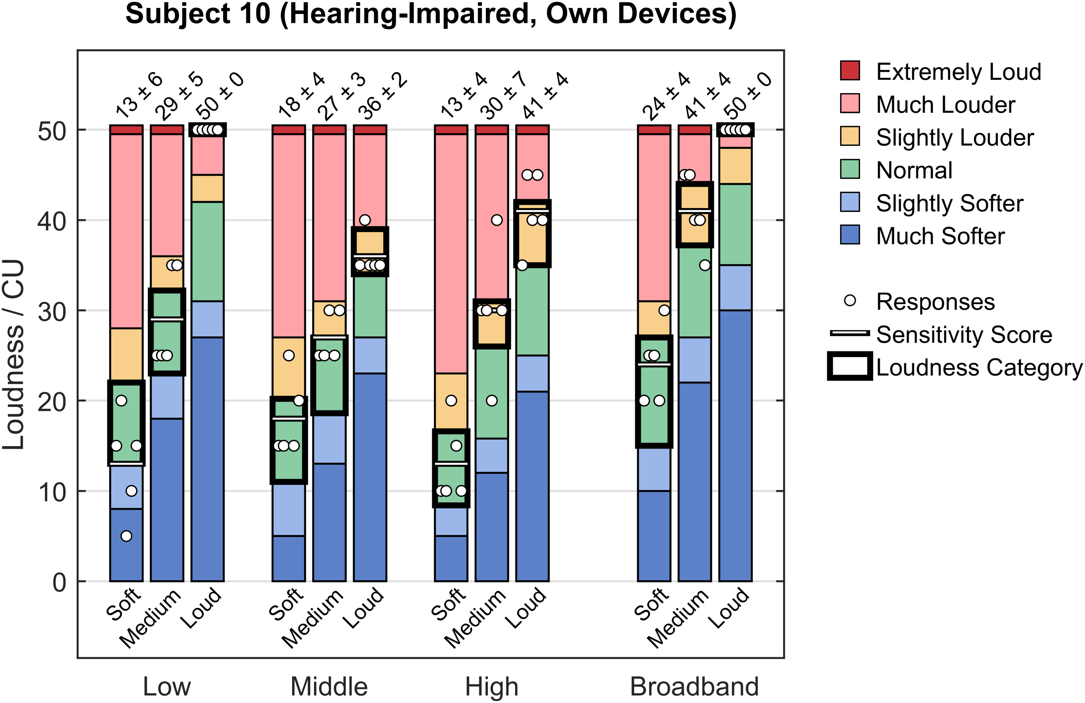
Example responses of one aided hearing-impaired subject with their own devices for a complete test run, along with the category-specific ranges of the color-coded loudness perception categories. Each bar is labeled with the mean and standard deviation of the corresponding responses (in CU). Additionally, the resulting sensitivity scores and loudness perception categories (“colors”) are highlighted for each presentation category. Note that the width of the loudness perception category extremely loud (dark red; S = 50 CU) is exaggerated slightly to make it visible in the plot.

Figure 6.

Example of loudness map for one aided hearing-impaired subject with their own devices (same data as shown in Figure 5). LVM frequency categories are shown along the horizontal axis, while LVM level categories can be seen along the vertical axis. The color-coded tiles correspond to the resulting category-specific loudness perception for this subject. This represents the standard LVM result display as shown to the hearing care professional. Note the references to frequency ranges (“200–920” etc., in Hz) and to level-dependent gain functions (“G50” etc.) that are intended to aid the hearing care professional in translating the LVM results into concrete actions for gain adjustments in the hearing aid fitting software.

Evaluation and Results

Several evaluation studies, both qualitative and quantitative, were subsequently conducted to assess the validity and practical usefulness of the method. First, details on the test subjects and measurement conditions are given below; then, the findings of a qualitative evaluation of the LVM are presented, followed by the results of two statistical investigations.

Subjects and Measurement Conditions

Two groups of test subjects were used in the evaluations. The first group consisted of normal-hearing subjects (N = 33); this was the original sample from which the LVM reference values had been derived (see above). The second group comprised adult hearing-impaired subjects (N = 30; 12 female and 18 male) aged between 65 and 89 years (median age: 81.5 years), with symmetrical hearing loss, whose audiograms met the conditions either for types N₂, N₃, or N₄ (mild, moderate, or moderate/severe category from the flat and moderately sloping group) or for type S₂ (mild category from the steep sloping group) according to Bisgaard et al. (2010). All hearing-impaired subjects were hearing aid users with between 3 and 48 years of experience (median: 10.5 years). Altogether, the following four measurement conditions were then defined:

Normal-hearing: Measurements with normal-hearing subjects without hearing aids.

Hearing-impaired (unaided): Measurements with hearing-impaired subjects without hearing aids.

Hearing-impaired (first fit): Measurements with hearing-impaired subjects fitted binaurally with either one of two state-of-the-art, commonly prescribed commercial hearing aids by two different manufacturers, using the manufacturers’ respective proprietary fitting formulas (15 subjects in each group; results were then pooled after an informal inspection did not reveal any differences relevant in the present context).

Hearing-impaired (own devices): Measurements with hearing-impaired subjects instructed to wear their own (binaurally fitted) hearing aids with the same settings that they used in everyday life.

Qualitative Evaluation

Having finalized the development of the LVM as reported above, the method was first put to the test in a variety of contexts with the aim of evaluating qualitatively whether it was suited to fulfill its intended purpose. Figure 7 shows examples of loudness maps from three different measurement conditions that illustrate very clearly the advantages of the method.

Figure 7.

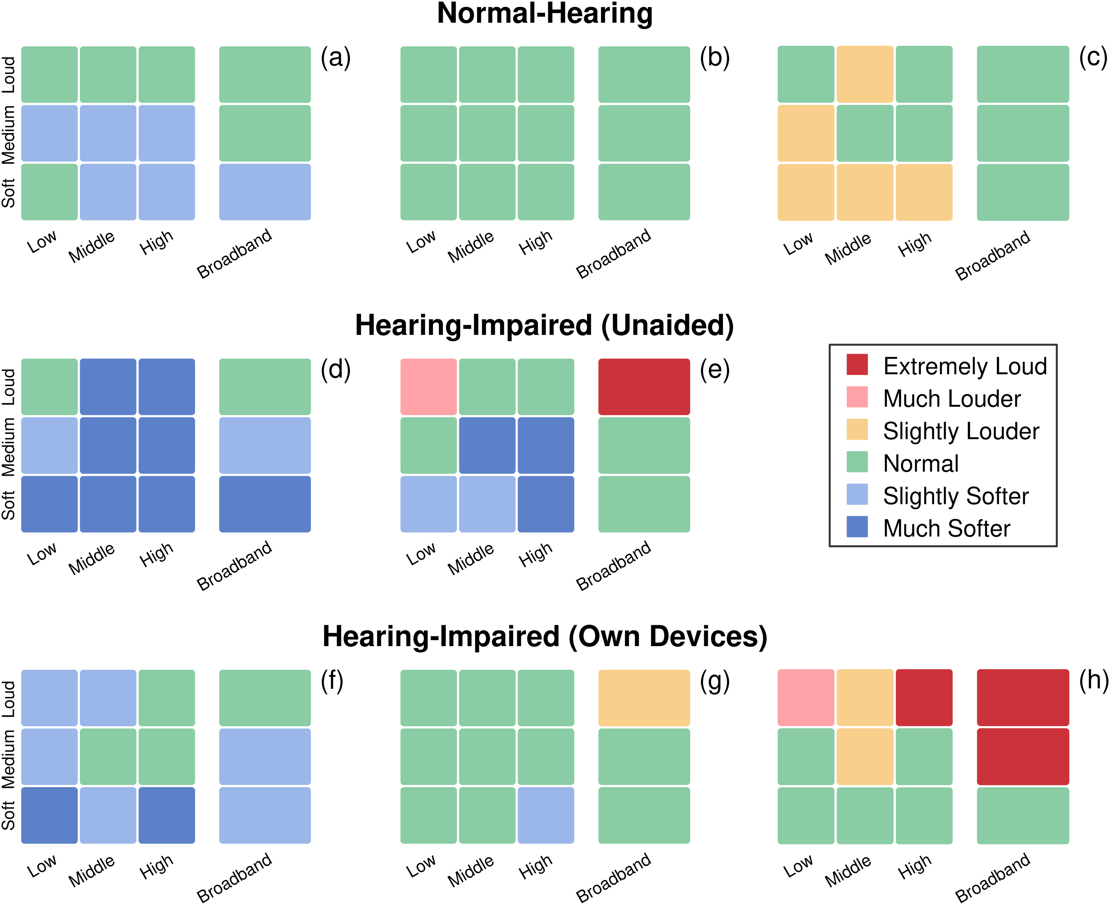
Examples of loudness maps for eight different subjects from three groups. Top row: results for three normal-hearing reference subjects (a, b, c); middle row: results for two unaided hearing-impaired subjects (d, e); bottom row: results for three aided hearing-impaired subjects with their own devices (f, g, h). See text for details.

The top row of Figure 7 shows loudness maps for three normal-hearing subjects. While Subject (b) has a completely green loudness map, corresponding to normal loudness perception in all 12 presentation categories (tiles), Subject (a) is a bit less sensitive, with a few tiles in the slightly softer (light blue) loudness perception category. Subject (c), on the other hand, is a bit more sensitive, showing a few yellow tiles, thus indicating that in some of the categories, stimuli were perceived as louder than normal (remember that due to the definitions of the boundaries of the loudness perception categories, ∼ 20% of normal-hearing results in any sample will be expected to be either slightly softer or slightly louder).

In the middle row of Figure 7, loudness maps for unaided hearing-impaired subjects are presented. Overall, Subjects (d) and (e) have very similar maps, with a few green tiles (normal) and many light blue (slightly softer) and even dark blue (much softer) tiles, reflecting their untreated hearing impairment. However, there is a striking difference between the two: Subject (d) is generally less sensitive at all levels, whereas Subject (e) is less sensitive than normal at low and medium levels, but considerably more sensitive at high levels, as evidenced by the occurrence of a light red tile (in the low loud category) and even a dark red tile (in the broadband loud category). This example is particularly interesting in that it illustrates the sensitivity of the method for cases like Subject (e), presumably with a strong loudness summation (Oetting et al., 2016). To illustrate this, Figure 8 shows the pure-tone audiograms (air conduction hearing threshold levels and uncomfortable loudness levels) for Subjects (d) and (e) from Figure 7. Both subjects have a similar audiometric hearing loss. The light red and dark red tiles in the loudness map of Subject (e), however, are a clear indication of a problematically sensitive loudness perception, especially in the broadband loud category, which is representative of the “speech in loud environments” situation that is critical for many hearing aid users.

Figure 8.

Pure-tone audiograms (air conduction hearing threshold levels and uncomfortable loudness levels) for Subjects (d) and (e) from Figure 7. The pure-tone average (PTA) at 500, 1,000, 2,000, and 4,000 Hz is 48.8 dB HL (right ear) and 50.0 dB HL (left ear), respectively, for Subject (d) versus 41.3 dB HL (right ear) and 45.0 dB HL (left ear), respectively, for Subject (e). All four audiograms correspond to type N₃ (moderate category from the flat and moderately sloping group) according to Bisgaard et al. (2010).

Finally, in the bottom row of Figure 7, loudness maps for three hearing-impaired subjects equipped with their own hearing aids are shown. This set of maps illustrates the primary use case of the LVM, namely the assessment (validation) of an existing hearing aid fitting. The map for Subject (g) shows a loudness map that corresponds to normal-hearing loudness perception. The map for Subject (f), on the other hand, suggests that loudness was softer than normal, especially at (but not limited to) low input levels. Subject (h), finally, shows close-to-normal loudness compensation for low input levels, but excessive loudness perception at middle and, especially, high input levels.

Quantitative Evaluation

Following the qualitative evaluation of the method, examples of which were reported in the previous section, the overall results from the four measurement conditions as defined above were analyzed quantitatively. Figure 9 shows bar charts of the total proportions of the six LVM loudness perception categories (“tile colors”) over all measurements for each measurement condition.

Figure 9.

Bar charts of the total proportions of the six color-coded Loudness Validation Method (LVM) loudness perception categories for four measurement conditions. Top left panel: normal-hearing reference subjects; top right panel: unaided hearing-impaired subjects; bottom left panel: aided hearing-impaired subjects with the first fit; bottom right panel: aided hearing-impaired subjects with their own devices.

Firstly, the results for the normal-hearing measurement condition (top left panel of Figure 9) are as expected, since this group is the reference group used to derive the values for the loudness category boundaries: There are no dark blue tiles (much softer) and roughly 10% light blue (slightly softer), 80% green (normal), and 10% yellow tiles (slightly louder), respectively. Furthermore, there is a small proportion of light red (much louder) and dark red tiles (extremely loud), reflecting the fact that especially sensitive normal-hearing subjects were excluded from the calculation of the category boundaries for the loud level categories (see above).

Secondly, the results for the hearing-impaired (unaided) condition are also as expected: The distribution is strongly skewed towards the softer categories (light blue and dark blue), which reflects the altered loudness perception of the unaided subjects with hearing loss. Additionally, a small proportion of light red and dark red tiles occur even in this group, which is presumably attributable to a particularly strong loudness summation effect in some subjects (Oetting et al., 2016). In other words, this illustrates that a certain proportion of unaided hearing-impaired subjects perceive the respective signals as louder than most normal-hearing subjects.

Thirdly, in the hearing-impaired (first fit) condition, an approximation to the normal-hearing distribution can be observed. Specifically, the proportion of softer categories (dark blue and light blue) is smaller compared to the unaided case, with green tiles making up the largest proportion of the results. However, the overall shift towards the normal (green) and slightly louder (yellow) categories has obviously also resulted in considerably higher proportions of light red and even dark red tiles, which might be undesirable, as it likely corresponds to uncomfortably loud perception in real-life situations.

Finally, the hearing-impaired (own devices) condition shows a shift towards the softer categories (in other words, “fewer red tiles, more blue tiles”) as compared to the first-fit case, which suggests a gain reduction in the fine-tuning phase of the hearing aid fitting. This results in a situation with gain settings at low input levels leading to a loudness perception that is much softer than normal (i.e., dark blue) for 9.4% of the subjects, while high input levels still result in louder-than-normal loudness perception in a substantial proportion of cases.

To investigate the respective influences of the various measurement conditions in more detail, the results were then analyzed statistically. For this purpose, an analysis of variance (ANOVA) was carried out on the normal-hearing versus hearing-impaired (first fit) conditions as well as on the normal-hearing vs. hearing-impaired (own devices) conditions, using R (Version 4.3.2).

Normal-Hearing Versus Hearing-Impaired (First Fit)

First, a two-way mixed ANOVA (with type III sums of squares) was carried out to examine the effects of measurement condition (normal-hearing vs. hearing-impaired [first fit]) and presentation category (low soft, low medium, etc.) on the LVM responses (more precisely, the sensitivity scores). Since the groups in the two measurement conditions consisted of different subjects, the model contained one between-subjects factor (measurement condition, with two levels) and one within-subjects factor (presentation category, with 11 levels). Note that one category (broadband loud) was excluded from the analysis due to the presence of a ceiling effect (defined as > 15% maximum responses, i.e., 50 CU, per category; McHorney & Tarlov, 1995) in the first-fit condition (15 out of 30 responses, i.e., 50.0%).

Applying Greenhouse-Geisser corrections to the degrees of freedom (ε = .47 for the main effect of category and for the Condition × Category interaction effect) to account for violations of the assumption of sphericity, the main effect of category was both significant and large, F(4.73, 288.40) = 486.95, p < .001, $η_{p}^{2}$ = 0.89 (trivially so, since the presentation categories were designed to be different from each other). While the main effect of condition was non-significant, F(1, 61) = 0.0004, p = .99, there was a significant interaction effect of Condition × Category on the LVM sensitivity scores, F(4.73, 288.40) = 9.99, p < .001, $η_{p}^{2}$ = 0.14, indicating a relatively large effect.

Figure 10 (top panel) shows box plots with the results of post-hoc pairwise comparisons (t tests with Holm-corrected p values) that were subsequently performed to investigate the nature of the interaction between measurement condition and presentation category (see below for a discussion and interpretation of the results).

Figure 10.

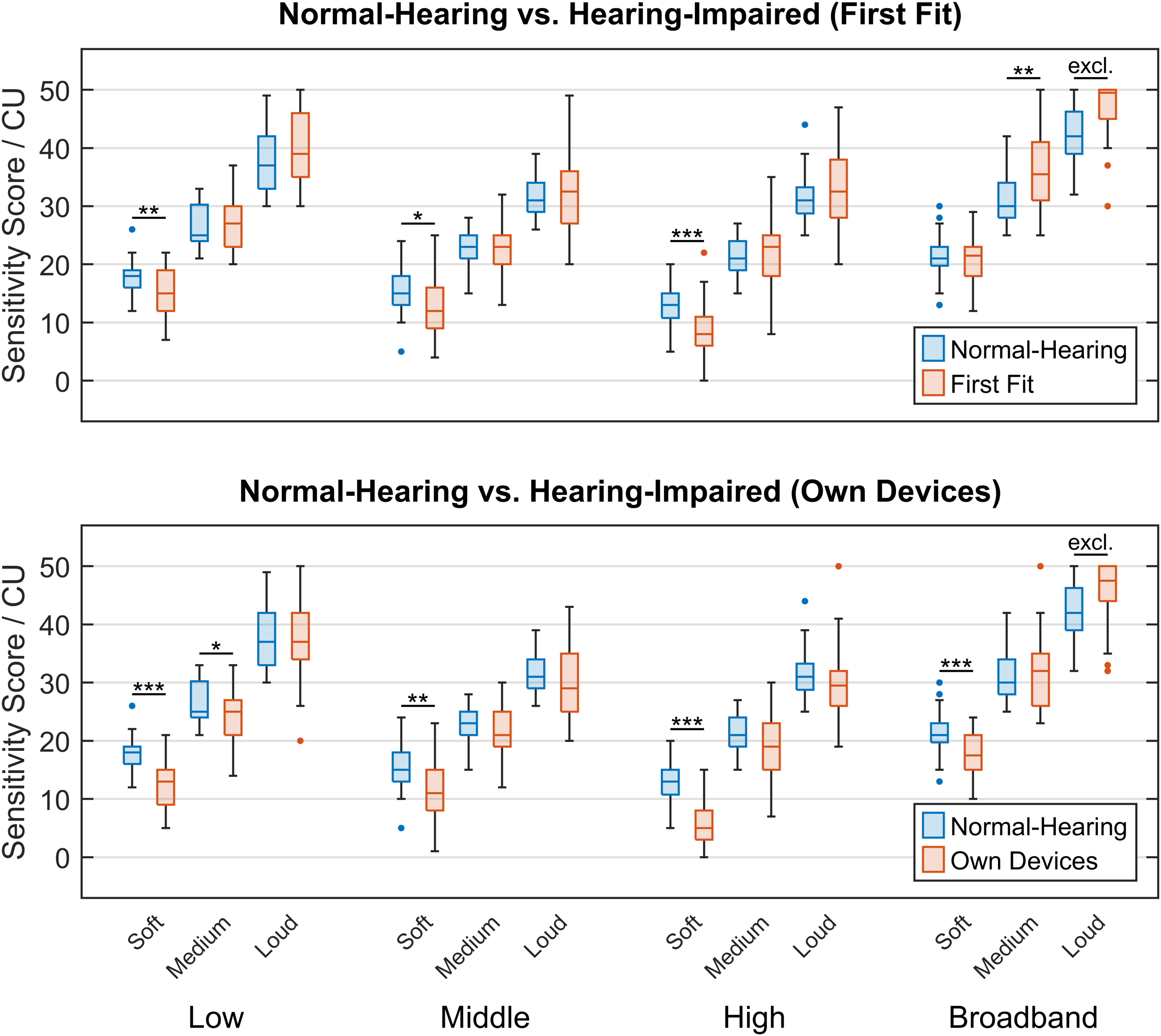
Box plots of sensitivity scores across presentation categories. Top panel: normal-hearing reference subjects (N = 33) versus hearing-impaired subjects with the first fit (N = 30); bottom panel: normal-hearing reference subjects (N = 33) versus hearing-impaired subjects with their own devices (N = 30). For each presentation category, pairwise comparisons were conducted between the two groups of subjects (***: p < .001, **: p < .01, *: p < .05, excl.: excluded due to ceiling effect).

Normal-Hearing Versus Hearing-Impaired (Own Devices)

Similarly, an equivalent two-way mixed ANOVA was carried out to investigate the effects of condition (this time, normal-hearing vs. hearing-impaired [own devices]) and category on the LVM sensitivity scores. Again, one category (broadband loud) was excluded from the analysis because of a ceiling effect in the own-devices condition (nine out of 30 responses, i.e., 30.0%).

To account for violations of the assumption of sphericity, Greenhouse-Geisser corrections were again applied to the degrees of freedom (ε = .53 for the main effect of category and for the Condition × Category interaction effect). The main effect of category was (again, trivially) significant and large, F(5.28, 322.20) = 492.24, p < .001, $η_{p}^{2}$ = 0.89, and the main effect of condition was also significant, F(1, 61) = 7.85, p = .007, $η_{p}^{2}$ = 0.11, corresponding to a medium effect. As before, there was a significant interaction effect of Condition × Category on the LVM sensitivity scores, F(5.28, 322.20) = 8.32, p < .001, $η_{p}^{2}$ = 0.12, this time indicating a medium effect.

Figure 10 (bottom panel) shows the corresponding box plots with the results of post-hoc pairwise comparisons (t tests with Holm-corrected p values) performed to look more closely into the interaction between measurement condition and presentation category. In the following section, the statistical findings will be discussed and interpreted in more detail.

Discussion

Looking at the top panel of Figure 10 (normal-hearing subjects vs. hearing-impaired subjects with first fit), the statistical analysis reveals that on average, in the narrowband (i.e., low, middle, and high) frequency categories, the hearing-impaired subjects with first fit perceived the stimuli from the soft level categories (i.e., low soft, middle soft, and high soft) as significantly softer than the normal-hearing subjects, while the medium and loud level categories show close-to-normal loudness perception. In the broadband case, on the other hand, the soft level category is close to normal, while the stimuli from the medium and loud level categories were perceived as louder than normal. The broadband loud level category even shows a ceiling effect (see above), indicating that for the first-fit condition, excessive broadband loudness perception becomes more pronounced as the input level increases. The results thus support the interpretation discussed in connection with Figure 9, namely that the amplification of low-level input signals relative to that of medium and high-level input signals is too low. A possible strategy for the hearing care professional to address this problem would be to increase the G₅₀ gain function while leaving G₆₅ and G₈₀ unchanged, which is one way of realizing wide dynamic range compression (WDRC; Dillon, 2012).

The bottom panel of Figure 10 (normal-hearing subjects vs. hearing-impaired subjects with their own devices) shows a similar overall pattern for the narrowband frequency categories as in the normal-hearing versus first-fit case (top panel): The soft level categories are perceived as significantly softer than normal by the hearing-impaired subjects with their own devices, whereas the medium and loud level categories are for the most part acceptable, with only one exception (low medium, which is softer than normal). For broadband stimuli, on the other hand, the soft level category is now significantly softer than normal, while the medium level category is close to normal, and the loud level category is still louder than normal (to the point of still showing a ceiling effect). Quantitatively, all categories in the own-devices condition show sensitivity score values that are shifted towards even lower sensitivity scores than in the first-fit condition. All these observations are consistent with the interpretation that as a tendency, an overall gain reduction has been used as a remedy for a broadband loud category with excessive loudness, at the cost of reducing the loudness of the soft level categories even further.

Thus, the statistical analyses support the insights gained from Figure 9. As a general observation, it can be stated that at least for this sample of subjects, fine-tuning has apparently not led to a change from the first fit towards normal-hearing loudness perception. This is in line with the findings of Caswell-Midwinter and Whitmer (2021), who showed that hearing aid fitting and fine-tuning based on the hearing aid users explicitly describing their perceived deficits are often inconsistent and unreliable. It is here that a method like the LVM can provide a tool to hearing care professionals for validating the subjective loudness perception with an existing fit without having to rely on the hearing aid users’ capacity for introspection, abstraction, and verbalization.

In addition, the LVM can help to identify the technical limitations of hearing aids. A particularly common example of this is light red or even dark red tiles in the loudness maps of unaided hearing-impaired subjects, reflecting excessive loudness perception in certain conditions (typically either low or broadband loud input signals) even without a hearing aid. The obvious solution in such cases would be the use of higher dynamic range compression ratios in the devices, and/or “negative gain” (i.e., attenuative coupling). However, in many cases, such measures are not technically possible to a sufficient degree. Hearing care professionals may then find it helpful when a tool such as the LVM provides guidance as to whether the solution can be found in the fine-tuning phase or rather in the search for better-suited devices or acoustic coupling.

In the context of the development of the NAL-NL2 fitting method, Keidser et al. (2012) found that the loudness adaptation of new hearing aid users with higher degree of hearing loss was not yet completed after 13 months of hearing aid usage. Considering this, the LVM could also be used as a tool for the assessment of loudness adaptation by repeating the measurement at specified intervals following the initial fit.

In its current state, the LVM validates the subjective perception of loudness using five test stimuli in each of the 12 presentation categories. To further shorten the measurement duration, it is conceivable that an analysis of appropriate datasets could reveal correlations between presentation categories such that the results from specific categories can be predicted from the results of other categories with sufficient reliability. Predictable categories could then be dispensed with, thus resulting in an even faster procedure. Furthermore, the number of stimuli per category could also be adaptively reduced, for example, if the first responses in a given presentation category all fall into the same loudness perception category (“color”).

Finally, as explained above, an optimization strategy designed to handle the ceiling effect observed in the loud level categories for the normal-hearing reference group was applied to the loudness perception category boundaries, resulting in more slightly louder (yellow) and much louder (light red) test results. However, other strategies are also possible in future versions of the LVM. For instance, to avoid ceiling effects, a lower presentation level for the stimuli from the loud level categories could be chosen. Another approach would be to select the test stimuli in such a way that ceiling effects occur less often, which might make any optimization obsolete in the first place.

Summary and Conclusions

In this article, we have presented a new method for validating loudness by detecting and quantifying deviations of an individual’s loudness perception from a normal-hearing reference. In contrast to other loudness measurement methods, the LVM uses carefully selected natural signals as stimuli, thus seeking to increase ecological validity given the technical conditions typically available to hearing care professionals. As a free-field suprathreshold measurement method, it can capture important effects relevant to the subjects’ real-life experience, such as loudness summation. It is particularly suited for aided measurements, specifically for the validation of an existing hearing aid fitting. As a tool for hearing care professionals, it can thus offer concrete help and orientation in fine-tuning and troubleshooting, rendering the process more efficient. Moreover, the method was rated by hearing care professionals to be fast, intuitive, and easily interpretable.

Qualitative evaluations confirmed that the phenomena typically encountered when dealing with hearing impairment and hearing aid fitting were captured well by the LVM. For instance, the method allows for identifying an individual’s “problem areas” (i.e., either insufficient or excessive loudness sensitivity) in the frequency and level dimensions with a resolution that is directly translatable into concrete actions in terms of gain adjustments. Furthermore, suprathreshold challenges for hearing aid fitting like, for example, loudness summation effects are immediately visible in the result display (the loudness map), as are possible improvements to an existing fitting strategy (regarding, e.g., closed coupling or dynamic range compression).

Finally, subsequent statistical evaluations were conducted over larger samples of individuals in different conditions (normal-hearing; unaided hearing-impaired; hearing-impaired with the first fit; and hearing-impaired with their own devices). These analyses showed the usefulness of the LVM for identifying, characterizing, and assessing existing larger-scale, superindividual patterns of hearing aid fitting.

Overall, we conclude that the LVM yields qualitatively plausible results that are both easily interpretable and practically helpful in the sense that the method enables hearing care professionals to derive concrete recommendations for action. It thus fills a gap between existing fitting methods and tools by helping to efficiently provide hearing aid users with the optimal gains and, in addition, thereby creating the basis for features like noise reduction or beamforming to develop their full potential. We therefore believe that the LVM can be particularly helpful in real-life settings where a sensible compromise between precision, robustness, time-efficiency, and ease of application is of the essence.

Supplemental Material

sj-xlsx-1-tia-10.1177_23312165241299778 - Supplemental material for Development and Evaluation of a Loudness Validation Method With Natural Signals for Hearing Aid Fitting

Supplemental material, sj-xlsx-1-tia-10.1177_23312165241299778 for Development and Evaluation of a Loudness Validation Method With Natural Signals for Hearing Aid Fitting by Mats Exter, Theresa Jansen, Laura Hartog and Dirk Oetting in Trends in Hearing

Footnotes

Acknowledgments

We would like to thank Annika Meyer-Hilberg for her help in selecting and analyzing the signals used in the LVM, and Amelie Hoffmann for her contributions to the optimization and evaluation of the method. Our thanks also go to our audiology team for conducting the evaluation measurements as well as for valuable discussions and feedback, and to the many hearing care professionals who shared their experiences with us when testing the LVM. Finally, we are very grateful to the associate editor, Michael A. Stone, and two anonymous reviewers for their detailed and helpful comments on an earlier version of this article.

Data Availability Statement

The data collected and analyzed as part of this study are provided as supplementary material to this article.

Declaration of Conflicting Interests

The author(s) declared the following potential conflicts of interest with respect to the research, authorship, and/or publication of this article: The authors declare that the research described in this article was conducted in connection with their employment at Hörzentrum Oldenburg gGmbH, which plans to offer the LVM as a software product under the name “revoloud.”

Funding

The authors disclosed receipt of the following financial support for the research, authorship, and/or publication of this article: This study was supported by the German Bundesministerium für Wirtschaft und Klimaschutz (BMWK, Federal Ministry for Economic Affairs and Climate Action), Project ID 49VF210055, INNO-KOM Project “AHOI”; and by the Deutsche Forschungsgemeinschaft (DFG, German Research Foundation), Project ID 352015383, SFB 1330 Project C4.

ORCID iDs

Mats Exter

Theresa Jansen

Laura Hartog

Dirk Oetting

Supplemental Material

Supplemental material for this paper is available online.

Appendix

Table A1 gives a description of the final set of signals used as stimuli in the LVM. As explained in the text, because of the rigorous criteria for eligibility of a signal as a test stimulus, only 50 out of the 60 signals in the table are unique (six signals appear in two different level categories each, while two signals appear in all three level categories for the respective frequency category).

References

Aazh

Moore

B. C. J.

(2007). The value of routine real ear measurement of the gain of digital hearing aids. Journal of the American Academy of Audiology, 18(8), 653–664. https://doi.org/10.3766/jaaa.18.8.3

Allen

J. B.

Hall

J. L.

Jeng

P. S.

(1990). Loudness growth in ½-octave bands (LGOB) – A procedure for the assessment of loudness. The Journal of the Acoustical Society of America, 88(2), 745–753. https://doi.org/10.1121/1.399778

American Speech-Language-Hearing Association (ASHA). (1998). Guidelines for hearing aid fitting for adults. American Journal of Audiology, 7(1), 5–13. https://doi.org/10.1044/1059-0889.0701.05

Arieh

Marks

L. E.

(2011). Measurement of loudness, part II: Context effects. In Florentine

Popper

A. N.

Fay

R. R.

(Eds.), Loudness (pp. 57–87). Springer. https://doi.org/10.1007/978-1-4419-6712-1_3

Bisgaard

Vlaming

M. S. M. G.

Dahlquist

(2010). Standard audiograms for the IEC 60118-15 measurement procedure. Trends in Amplification, 14(2), 113–120. https://doi.org/10.1177/1084713810379609

Brand

Hohmann

(2002). An adaptive procedure for categorical loudness scaling. The Journal of the Acoustical Society of America, 112(4), 1597–1604. https://doi.org/10.1121/1.1502902

British Broadcasting Corporation (BBC). (1984). BBC sound effects [CD set].

Byrne

(1996). Hearing aid selection for the 1990s: Where to? Journal of the American Academy of Audiology, 7(6), 377–395. https://pubmed.ncbi.nlm.nih.gov/8972440/

Byrne

Dillon

Tran

Arlinger

Wilbraham

Cox

Hagerman

Hetu

Kei

Lui

Kiessling

Kotby

M. N.

Nasser

N. H. A.

El Kholy

W. A. H.

Nakanishi

Oyer

Powell

Stephens

Meredith

, … Ludvigsen

(1994). An international comparison of long-term average speech spectra. The Journal of the Acoustical Society of America, 96(4), 2108–2120. https://doi.org/10.1121/1.410152

10.

Caswell-Midwinter

Whitmer

W. M.

(2021). The perceptual limitations of troubleshooting hearing-aids based on patients’ descriptions. International Journal of Audiology, 60(6), 427–437. https://doi.org/10.1080/14992027.2020.1839679

11.

Cornelisse

L. E.

Seewald

R. C.

Jamieson

D. G.

(1995). The input/output formula: A theoretical approach to the fitting of personal amplification devices. The Journal of the Acoustical Society of America, 97(3), 1854–1864. https://doi.org/10.1121/1.412980

12.

Cox

R. M.

Alexander

G. C.

(1995). The Abbreviated Profile of Hearing Aid Benefit. Ear and Hearing, 16(2), 176–186. https://doi.org/10.1097/00003446-199504000-00005

13.

Cox

R. M.

Alexander

G. C.

Taylor

I. M.

Gray

G. A.

(1997). The Contour Test of loudness perception. Ear and Hearing, 18(5), 388–400. https://doi.org/10.1097/00003446-199710000-00004

14.

Cox

R. M.

Gray

G. A.

(2001). Verifying loudness perception after hearing aid fitting. American Journal of Audiology, 10(2), 91–98. https://doi.org/10.1044/1059-0889(2001/009)

15.

Dermody

Byrne

(1975). Loudness summation with binaural hearing aids. Scandinavian Audiology, 4(1), 23–28. https://doi.org/10.3109/01050397509075010

16.

Deutsches Institut für Normung (DIN). (2009). Measurement technique for the simulation of the auditory sensation of sharpness (DIN 45692:2009-08). https://doi.org/10.31030/1521326

17.

Deutsches Institut für Normung (DIN). (2010). Calculation of loudness level and loudness from the sound spectrum – Zwicker method – Amendment 1: Calculation of the loudness of time-variant sound (DIN 45631/A1:2010-03). https://doi.org/10.31030/1555185

18.

Dillon

(2012). Hearing aids (2nd ed.). Boomerang Press.

19.

European Hearing Instrument Manufacturers Association (EHIMA). (2022). EuroTrak Germany 2022 . https://www.ehima.com/wp-content/uploads/2022/06/EuroTrak_Germany_2022.pdf

20.

Fastl

Zwicker

(2007). Psychoacoustics: Facts and models (3rd ed.). Springer. https://doi.org/10.1007/978-3-540-68888-4

21.

Genesis. (2012, April). Loudness Toolbox (Version 1.2) [Computer software]. Retrieved January 22, 2024, from https://web.archive.org/web/20190509124114/http://genesis-acoustics.com/en/pages/post/sonie.php

22.

Heeren

Hohmann

Appell

J. E.

Verhey

J. L.

(2013). Relation between loudness in categorical units and loudness in phons and sones. The Journal of the Acoustical Society of America, 133(4), EL314–EL319. https://doi.org/10.1121/1.4795217

23.

Heller

(1985). Hörfeldaudiometrie mit dem Verfahren der Kategorienunterteilung (KU). Psychologische Beiträge, 27, 478–493.

24.

Hoffmann

(2021). Optimierung und Evaluation der Lautheitsverifikationsmethode in der Hörgeräte-Anpassung [Unpublished bachelor’s thesis]. Jade Hochschule Wilhelmshaven/Oldenburg/Elsfleth, Germany.

25.

Holube

(2011). Speech intelligibility in fluctuating maskers. Proceedings of the International Symposium on Auditory and Audiological Research, 3, 57–64. https://proceedings.isaar.eu/index.php/isaarproc/article/view/2011-06

26.

Hörzentrum Oldenburg. (2024, January 22). Oldenburg Measurement Applications [Computer software]. https://www.hz-ol.de/en/oma.html

27.

International Organization for Standardization (ISO). (2003). Acoustics – Normal equal-loudness-level contours (ISO 226:2003). https://www.iso.org/standard/34222.html

28.

International Organization for Standardization (ISO). (2006). Acoustics – Loudness scaling by means of categories (ISO 16832:2006). https://www.iso.org/standard/32442.html

29.

Jansen

(2020). Entwicklung und Evaluation eines Verfahrens zur Bestimmung der Lautheitswahrnehmung von Hörgeräteträgern für natürliche Signale [Unpublished bachelor’s thesis]. Jade Hochschule Wilhelmshaven/Oldenburg/Elsfleth, Germany.

30.

Jansen

Hartog

Hansen

Oetting

(2020, September 3–4). Entwicklung und Evaluation eines Verfahrens zur Bestimmung der Lautheitswahrnehmung von Hörgeräteträgern für natürliche Signale [Poster presentation]. 23. Jahrestagung der Deutschen Gesellschaft für Audiologie, Cologne, Germany. https://doi.org/10.3205/20dga183

31.

Jansen

Krueger

Hartog

Oetting

(2021, August 23–27). Development and evaluation of a method to determine the loudness perception of hearing aid users for natural signals [Poster presentation]. 8th International Symposium on Auditory and Audiological Research. https://isaar.eu/programme-book/

32.

Jenstad

L. M.

Cornelisse

L. E.

Seewald

R. C.

(1997). Effects of test procedure on individual loudness functions. Ear and Hearing, 18(5), 401–408. https://doi.org/10.1097/00003446-199710000-00005

33.

Jenstad

L. M.

Van Tasell

D. J.

Ewert

(2003). Hearing aid troubleshooting based on patients’ descriptions. Journal of the American Academy of Audiology, 14(7), 347–360. https://doi.org/10.1055/s-0040-1715754

34.

Keidser

Dillon

Carter

O’Brien

(2012). NAL-NL2 empirical adjustments. Trends in Amplification, 16(4), 211–223. https://doi.org/10.1177/1084713812468511

35.

Keidser

Dillon

Flax

Ching

Brewer

(2011). The NAL-NL2 prescription procedure. Audiology Research, 1(1), Article e24. https://doi.org/10.4081/audiores.2011.e24

36.

Keidser

Seymour

Dillon

Grant

Byrne

(1999). An efficient, adaptive method of measuring loudness growth functions. Scandinavian Audiology, 28(1), 3–14. https://doi.org/10.1080/010503999424860

37.

Kiessling

Schubert

Archut

(1996). Adaptive fitting of hearing instruments by category loudness scaling (ScalAdapt). Scandinavian Audiology, 25(3), 153–160. https://doi.org/10.3109/01050399609047998

38.

Killion

M. C.

Fikret-Pasa

(1993). The 3 types of sensorineural hearing loss: Loudness and intelligibility considerations. The Hearing Journal, 46(11), 31–36.

39.

Kochkin

(2011). MarkeTrak VIII: Reducing patient visits through verification & validation. The Hearing Review, 18(6), 10–12.

40.

Kramer

Schädler

M. R.

Hohmann

Oetting

, & Warzybok

(2020). Speech intelligibility and loudness perception with the trueLOUDNESS fitting rule. Proceedings of DAGA, 46, 114–117. https://pub.dega-akustik.de/DAGA_2020/data/articles/000354.pdf

41.

McHorney

C. A.

Tarlov

A. R.

(1995). Individual-patient monitoring in clinical practice: Are available health status surveys adequate? Quality of Life Research, 4(4), 293–307. https://doi.org/10.1007/BF01593882

42.

Moore

B. C. J.

(2000). Use of a loudness model for hearing aid fitting: IV: Fitting hearing aids with multi-channel compression so as to restore ‘normal’ loudness for speech at different levels. British Journal of Audiology, 34(3), 165–177. https://doi.org/10.3109/03005364000000126

43.

Moore

B. C. J.

Glasberg

B. R.

(1997). A model of loudness perception applied to cochlear hearing loss. Auditory Neuroscience, 3, 289–311.

44.

Moore

B. C. J.

Glasberg

B. R.

Stone

M. A.

(2010). Development of a new method for deriving initial fittings for hearing aids with multi-channel compression: CAMEQ2-HF. International Journal of Audiology, 49, 216–227. https://doi.org/10.3109/14992020903296746

45.

Oetting

Brand

Ewert

S. D.

(2014). Optimized loudness-function estimation for categorical loudness scaling data. Hearing Research, 316, 16–27. https://doi.org/10.1016/j.heares.2014.07.003

46.

Oetting

Hohmann

Appell

J.-E.

Kollmeier

Ewert

S. D.

(2016). Spectral and binaural loudness summation for hearing-impaired listeners. Hearing Research, 335, 179–192. https://doi.org/10.1016/j.heares.2016.03.010

47.

Oetting

Hohmann

Appell

J.-E.

Kollmeier

Ewert

S. D.

(2018). Restoring perceived loudness for listeners with hearing loss. Ear and Hearing, 39(4), 664–678. https://doi.org/10.1097/AUD.0000000000000521

48.

Palmer

C. V.

Mueller

H. G.

Moriarty

(1999). Profile of aided loudness: A validation procedure. The Hearing Journal, 52(6), 34, 36, 40–42. https://doi.org/10.1097/00025572-199906000-00004

49.

Ricketts

T. A.

(1996). Fitting hearing aids to individual loudness-perception measures. Ear and Hearing, 17(2), 124–132. https://doi.org/10.1097/00003446-199604000-00006

50.

Scollie

Seewald

Cornelisse

Moodie

Bagatto

Laurnagaray

Beaulac

Pumford

(2005). The desired sensation level multistage input/output algorithm. Trends in Amplification, 9(4), 159–197. https://doi.org/10.1177/108471380500900403

51.

Smeds

Keidser

Zakis

Dillon

Leijon

Grant

Convery

Brew

(2006a). Preferred overall loudness: I: Sound field presentation in the laboratory. International Journal of Audiology, 45(1), 2–11. https://doi.org/10.1080/14992020500190144

52.

Smeds

Keidser

Zakis

Dillon

Leijon

Grant

Convery

Brew

(2006b). Preferred overall loudness: II: Listening through hearing aids in field and laboratory tests. International Journal of Audiology, 45(1), 12–25. https://doi.org/10.1080/14992020500190177

53.

Souza

P. E.

(2002). Effects of compression on speech acoustics, intelligibility, and sound quality. Trends in Amplification, 6(4), 131–165. https://doi.org/10.1177/108471380200600402

54.

Valente

Van Vliet

(1997). The Independent Hearing Aid Fitting Forum (IHAFF) protocol. Trends in Amplification, 2(1), 6–35. https://doi.org/10.1177/108471389700200102

Supplementary Material

Please find the following supplemental material available below.

For Open Access articles published under a Creative Commons License, all supplemental material carries the same license as the article it is associated with.

For non-Open Access articles published, all supplemental material carries a non-exclusive license, and permission requests for re-use of supplemental material or any part of supplemental material shall be sent directly to the copyright owner as specified in the copyright notice associated with the article.

0.00 MB

0.07 MB