On the distribution of the number of phases per possession in 2025 Men's Six Nations rugby

Abstract

Data from the Men's 2025 Six Nations are analyzed to determine the number of possessions in a match and the distribution of the number phases per possession in international rugby. Each team can expect an average of 50 possessions in a match. The distribution is approximately geometric with the expected probability of possession being lost in any given phase of 0.365. Systematic deviations from the geometric distribution, however, showed phases in which the observed number of possession endings exceeded the expected counts. The discrete Weibull distribution reduced the number of deviations in which the observed number of counts exceeded the expected number. We conclude that the discrete Weibull distribution is more congruent with the distribution of the number of phases per possession. Under the discrete Weibull distribution, the value of expected probability can change (in this case, to decrease) methodically as the phases increase. This effect on the phases per possession is, we believe, a novel observation not previously described in the rugby literature. It is likely that the overall distribution results from the constraints imposed by of the Laws of the Game, Referee's interpretations, and, importantly, common overall coaching approaches to playing the game.

Introduction

A fundamental factor in the game of rugby union involves the number of phases a team plays-through each time the team has possession of the ball. Playing with possession allows a team to control the pace and tenor of a match, and unlike other sports – such as association football (soccer), gridiron (American) football, ice hockey, and basketball – it is only possible to score points in rugby when you have possession of the ball, however briefly. Understanding the distribution of the phases of play allows us to predict the likelihood of a team conceding possession early in a possession – by kicking the ball away as an example – or their ability to sustain multiple phases of play to attempt to disfigure the defense. These also bear on how their opponent chooses to defend. Knowledge of the distribution provides coaches information on how possible modifications to a team's attacking approach might enhance their success. The number of phases per possession can also inform strength and conditioning coaches with respect to the expected number of tackles and rucking events experienced by players, and may be useful to students of rugby performance indicators by further contextualizing their data.

All data distributions can be considered carriers of information (Jaynes, 2003: 117). The observed distribution is the result of random processes at work modified by constraints on the inputs. Most observed patterns result from simple constraints on information (Frank, 2009) and arise from aggregations of many small processes. We observe the distributions and, from them, begin to infer what the constraints might be (Frank, 2014). Jaynes (2003: 198) admonishes us to think of probability distributions in terms of their information content and, from that, to better understand how they developed.

Lisman and van Zuylen (1972) state that the most probable distribution of a stochastic variable is obtained by maximizing the entropy of its distribution under given constraints. Under these conditions, the resulting distribution is the one with the greatest uncertainty (Guiasu and Shenitzer, 1985), the least predictability, and the least bias (Harte, 2011: 22) given the constraints. In other words, following a maximum entropy distribution, the outcomes of a series of random events is the least predictable of all possible results under the imposed constraints.

Playing rugby using maximum entropy distributions is the most likely approach to maximize uncertainty in the defense. Maximum entropy theory has been applied successfully in many fields, including physics, biology, image resolution, and climate studies (Harte, 2011: 133). In rugby terms, by playing in a manner in which the choices of the attacker are governed by a maximum entropy distribution, the outcome of an attacking possession in terms of retaining or losing possession is the least predictable to the defense. Randomness generates uncertainty in the opponent while planned patterns of play results in predictability. Included in the category of maximum entropy distributions are the geometric and the Weibull distributions, described below.

Some generative processes produce unique outcomes and in other cases an equifinality of multiple possible processes can obscure which process is dominating. In large samples, the observed distributions tend towards the actual shape of the limiting distribution of the population from which the samples are taken. This is a manifestation of the central limit theorem and of entropy theory (van Campenhout and Cover, 1981). Modeling the distribution of large samples, therefore, may provide insight into the underlying processes at work.

Some definitions

In order to perform quantitative analyses of rugby it is necessary to define some terms. For the purposes of this study, we will define a possession in the following way:

A possession is defined to mean that a team has control of the ball while it is in play.

Having control of the ball means that the ball is in the hands of an attacking player; is in a scrum, a lineout, a tackle, a ruck, or a maul controlled (in the opinion of the Referee) by the attacking team; is being passed from one attacking player to another; or is in the air or on the ground following a kick or a passed ball by the attacking player. A ball on the ground is not controlled by the other team unless and until it is in the hands of one of its players. This allows a possession to continue unabated, for example, if the attacking team recovers the ball after a kick or if the ball is temporarily on the ground following a pass or a dropped ball that has not gone forward. It is not sufficient for an opponent merely to touch or deflect a ball for it to be in their control.

A ball being in play means that the Referee has allowed play to begin and has not indicated that a stoppage in play has occurred by blowing the whistle. As examples, at the beginning of each half of play, after the scoring of points, and at dropouts originating from the 22-meter line or the goal line, the kicking team is given control of the ball, but at that point it is not in play. These situations should not, therefore, be counted as a possession. These purely ministerial duties all occur while the ball is not in play and, in fact, the kicks themselves restart play.

A new possession begins whenever a team first gains control of the ball while it is in play. This can result, for instance, from being awarded a scrum or a lineout, because of an infringement by the opposition as determined by the Referee, or through turning the ball over in open play. A new possession can begin from several possible match scenarios, but always while the ball is in play. A possession ends when the team loses control of the ball, concedes control to the opposition, points are scored, or the Referee stops play.

Each possession can be divided into discrete episodes or phases of play. In this study we define a phase as follows:

A phase is defined as an episode of play consecutively numbered from the beginning of possession (first phase) to the last episode of play when possession ends.

We note that this is not the same the definition of this term as given by World Rugby (2025). Except for the first phase and the last phase, all phases typically begin and end when a tackle is made, a ruck forms, and the ball emerges to be played again. Phases can also end and the subsequent phase begins in open play when the Referee determines that a maul has formed and the ball emerges. The seemingly simple issue of determining when a phase ends and a new phase begins is often surprisingly difficult and somewhat subjective. Under the Laws of the Game, there is no generally-accepted set of guidelines of when there is a phase transition and making such a determination often involves a degree of observer (and Referee) interpretation. Two rational observers may well count a different number of phases in a possession. An example of this phenomenon is to observe the counts of the number of phases played, often provided real-time in videos of matches, and comparing those counts shown with your own counts of phases. Unfortunately, there is ultimately a degree of irreducible subjectivity in the counting of phases per possession. Experience has shown, however, that the differences are usually few in number and in magnitude, but they nevertheless do occur. A part of this study is devoted to a test of the reproducibility of the counts of the number of possessions that end in the various phases in one match (see below).

To illustrate the method of counting the number of phases in which possession ends we provide a few examples of typical rugby situations and how they translate into the data counts used in this study. Assume the following three relatively straightforward scenarios in which the Red team is playing the Blue team:

Red has been awarded a scrum. The ball is controlled in the scrum (possession begins and play is now in first phase) and emerges to be passed by the scrumhalf. The ball is subsequently passed to the center who is tackled by a Blue player (end of first phase). The ensuing ruck is won by Red (beginning of second phase) and the ball is kicked to touch. In this example the Red possession ended in the second phase of play.

Red is awarded a penalty and the kick is taken quickly through the mark (possession begins and we are in first phase). The Red player is tackled and the ball emerges to Red from the ensuing ruck (beginning of second phase). A Red player then passes the ball to another Red player but the pass is intercepted by a Blue player (end of the Red possession in the second phase and the beginning of a Blue possession) who successfully scores a try (the Blue possession ends with a try scored in first phase).

Red is awarded a lineout. The ball is thrown in and controlled by Red (possession begins and we are in first phase). The ball is passed out to the backline and kicked ahead by a center. The ball is caught after striking the ground by another Red attacker who runs forward with the ball and scores a try (the Red possession ends in first phase).

Possible scenarios can be simple or complex, but these three illustrate how the phase in which possession ended can be counted in a stepwise fashion to produce the phase distribution for analysis.

Characterization of phases and phases per possession

The number of possessions by each team in a match is quite variable, but casual observation of many matches suggests that approximately 50 possessions in a match are typical (in this study we test this hypothesis). The number of phases in a possession is similarly variable and can range from one to an indeterminate maximum based solely on the abilities of the team and the duration of the match. Based upon many years of watching rugby, a practical upper limit observed by the author is around 50 phases (a contemporary media report (Averis, 2015) indicated that Ireland played through 45 phases in one possession against Wales in the 2015 Six Nations competition). More than about 10 phases in a possession, however, is fairly rare. While published data are scarce, World Rugby (2023) data on the number of phases observed in the build-up to tries suggests that the median number of phases in a possession is typically between two and three.

The number of phases in a possession provides clues on how the game is played. Biscombe and Drewett (1998) argue that playing the game while emphasizing ball-retention and handling through multiple phases provides the attacking team opportunities to disfigure the defense and may lead to greater success. They suggest that playing through the phases was the typical approach taken in rugby towards the end of the twentieth century. There is also a school of thought that argues it is more advantageous to strike quickly via more of a power-game. If success is not achieved in the first few phases it might be preferable to play for territory and apply defensive pressure on the opponent to create opportunities to turn the ball over and attack again (for nontechnical media descriptions of this approach, see Kinsella, 2013, and Williamson, 2023).

A study of the number of phases per possession should cast light on the practical application of rugby theory. The shape of the distribution of the phases of possession observed in a large sample should reveal a form of ‘natural selection’ developed through trial and error to solve the problem of playing the game effectively, at least among the teams involved in the competition under consideration. The resulting distribution is expected to provide valuable clues about playing the game. At a minimum, we would not expect the chosen approach of playing the game to be highly inconsistent with the observed data. Consistency in the distributions among teams in the number of phases per possession should accurately reflect a common overall approach to the game.

Understanding the distribution of the phases of possession may also inform choices on how best to coach players to more effective approaches to the game. The primary goal of this study is to describe and interpret the distribution of the number of phases per possession in the 2025 Men's Six Nations.

Data and methods

Data for this study were obtained from all 15 matches of the 2025 Men's Six Nations, an annual competition played in Europe over about seven weeks in the spring of each year where each nation plays every other nation only once. Video of each match was analyzed by counting the number of possessions and the number of phases played within each possession. Data were collected by nation for each match and reported in three ways: the total counts of phases in which possession ended for both teams in each match (Table 1), the counts of each team's possessions and the number phases played by each team in all of its five matches (Table 2), and the aggregated counts of the number of occurrences of each phase in which possession ended by nation in all five of their matches (Table 3). In total, the data set includes 1495 possessions covering 4092 individual phases of play. All calculations were performed using a Microsoft^©Excel 2019 spreadsheet or using online calculators. Most probabilities, p-values, and coefficients of determination ( $r^2$ ) are reported to three decimal places. Standard statistical tests were performed using an α-level of 0.05 established a priori. Some data on the number of phases per possession from the 2023 Men's Six Nations were obtained from World Rugby (2023).

Table 1.

Counts of the phase in which possession ended in the 2025 Men's Six Nations arranged by match.

Round:	1	1	1	2	2	2	3	3	3	4	4	4	5	5	5
Match #:	1	2	3	4	5	6	7	8	9	10	11	12	13	14	15
Phase	Wal-Fra	Ita-Sco	Eng-Ire	Wal-Ita	Eng-Fra	Sco-Ire	Ire-Wal	Eng-Sco	Fra-Ita	Fra-Ire	Wal-Sco	Eng-Ita	Ire-Ita	Eng-Wal	Fra-Sco	Total	p
1	26	30	33	59	63	42	40	44	30	50	37	53	36	36	41	620	0.415
2	16	24	24	24	19	16	23	23	15	21	11	21	16	19	19	291	0.195
3	8	19	24	25	23	16	15	17	17	9	17	19	15	18	8	250	0.167
4	5	8	10	7	2	4	8	4	8	6	4	13	9	8	4	100	0.067
5	5	3	8	2	2	4	8	6	3	2	6	5	5	6	2	67	0.045
6	3	2	3	2	4	3	3	0	1	4	3	4	7	3	5	47	0.031
7	4	1	1	1	3	0	2	1	5	5	4	2	2	2	6	39	0.026
8	0	0	1	0	2	4	3	0	3	1	1	1	0	1	4	21	0.014
9	2	1	1	0	0	2	3	2	1	0	2	0	1	1	0	16	0.011
10	3	0	0	0	1	1	0	2	2	3	0	0	0	1	1	14	0.009
11	3	1	0	0	0	0	0	0	0	1	0	0	0	0	0	5	0.003
12	2	1	0	1	0	0	0	1	0	0	2	0	1	1	0	9	0.006
13	1	1	0	1	0	1	1	1	0	0	0	0	0	0	0	6	0.004
14	0	1	0	0	0	0	0	1	0	0	0	0	0	0	0	2	0.001
15	1	0	0	0	0	0	0	0	0	1	2	0	0	0	0	4	0.003
16	0	1	0	0	0	0	0	0	0	0	0	0	0	0	0	1	0.001
17	0	0	0	0	0	0	0	0	0	0	0	0	0	0	1	1	0.001
18	0	0	0	0	0	0	0	1	0	0	1	0	0	0	0	2	0.001
19	0	0	0	0	0	0	0	0	0	0	0	0	0	0	0	0	0.000
20	0	0	0	0	0	0	0	0	0	0	0	0	0	0	0	0	0.000
Total	79	93	105	122	119	93	106	103	85	103	90	118	92	96	91	1495	1.000
By Team	35/44	44/49	50/55	60/62	59/60	51/42	55/51	52/51	45/40	48/55	46/44	53/65	50/42	50/46	48/43

Notes: “Round” is the competition round in which the game was played. “Match #” is the order in which the matches were played through the competition. “Phase” is the phase in which each of the 1495 possessions ended. The column titled “Total” is the aggregated count of all phase endings in the competition. “p” is the proportion of occurrences of each phase ending. The row entitled “Total” is the total number of possessions observed in each match. The row entitled “By Team” shows the number of possessions by each team in each match (first team listed/second team listed).

Table 2.

Counts of the phase in which possession ended in the 2025 Men's Six Nations arranged by team and grouped into the five rounds of play.

Team:	England:					France:					Ireland:					Italy:					Scotland:					Wales:
Round: Phase	1	2	3	4	5	1	2	3	4	5	1	2	3	4	5	1	2	3	4	5	1	2	3	4	5	1	2	3	4	5	Total	p
1	13	32	22	18	16	15	31	13	26	25	20	19	21	24	21	16	35	17	35	15	14	23	22	16	16	11	24	19	21	20	620	0.415
2	13	9	15	15	13	11	10	8	13	11	11	11	12	8	8	13	12	7	6	8	11	5	8	4	8	5	12	11	7	6	291	0.195
3	13	12	11	5	10	6	11	10	2	4	11	6	9	7	8	7	11	7	14	7	12	10	6	11	4	2	14	6	6	8	250	0.167
4	3	1	1	7	5	2	1	2	2	0	7	1	5	4	2	4	1	6	6	7	4	3	3	0	4	3	6	3	4	3	100	0.067
5	5	0	2	2	2	2	2	3	0	1	3	1	4	2	3	1	1	0	3	2	2	3	4	3	1	3	1	4	3	4	67	0.045
6	2	1	0	4	1	1	3	1	0	2	1	1	2	4	4	1	1	0	0	3	1	2	0	1	3	2	1	1	2	2	47	0.031
7	0	3	0	2	2	2	0	4	2	4	1	0	1	3	2	0	0	1	0	0	1	0	1	3	2	2	1	1	1	0	39	0.026
8	0	1	0	0	1	0	1	1	0	1	1	2	1	1	0	0	0	2	1	0	0	2	0	0	3	0	0	2	1	0	21	0.014
9	1	0	0	0	0	2	0	1	0	0	0	0	0	0	1	1	0	0	0	0	0	2	2	2	0	0	0	3	0	1	16	0.011
10	0	0	0	0	0	0	1	2	2	0	0	1	0	1	0	0	0	0	0	0	0	0	2	0	1	3	0	0	0	1	14	0.009
11	0	0	0	0	0	2	0	0	1	0	0	0	0	0	0	0	0	0	0	0	1	0	0	0	0	1	0	0	0	0	5	0.003
12	0	0	0	0	0	0	0	0	0	0	0	0	0	0	1	1	0	0	0	0	0	0	1	1	0	2	1	0	1	1	9	0.006
13	0	0	0	0	0	1	0	0	0	0	0	0	0	0	0	0	1	0	0	0	1	1	1	0	0	0	0	1	0	0	6	0.004
14	0	0	1	0	0	0	0	0	0	0	0	0	0	0	0	0	0	0	0	0	1	0	0	0	0	0	0	0	0	0	2	0.001
15	0	0	0	0	0	0	0	0	0	0	0	0	0	1	0	0	0	0	0	0	0	0	0	2	0	1	0	0	0	0	4	0.003
16	0	0	0	0	0	0	0	0	0	0	0	0	0	0	0	0	0	0	0	0	1	0	0	0	0	0	0	0	0	0	1	0.001
17	0	0	0	0	0	0	0	0	0	0	0	0	0	0	0	0	0	0	0	0	0	0	0	0	1	0	0	0	0	0	1	0.001
18	0	0	0	0	0	0	0	0	0	0	0	0	0	0	0	0	0	0	0	0	0	0	1	1	0	0	0	0	0	0	2	0.001
19	0	0	0	0	0	0	0	0	0	0	0	0	0	0	0	0	0	0	0	0	0	0	0	0	0	0	0	0	0	0	0	0.000
20	0	0	0	0	0	0	0	0	0	0	0	0	0	0	0	0	0	0	0	0	0	0	0	0	0	0	0	0	0	0	0	0.000
Total	50	59	52	53	50	44	60	45	48	48	55	42	55	55	50	44	62	40	65	42	49	51	51	44	43	35	60	51	46	46	1495	1.000

Notes: “Team” is the nation under consideration. “Round” is the competition round in which the game was played. The column entitled “Total” is the aggregated number of observations of possession ending in that phase. “p” is the observed proportion of phase endings in that phase. The row entitled “Total” is the total number of possessions in each match in each round.

Table 3.

Counts of the phase in which possession ended for each Nation in the 2025 Men's Six Nations.

Counts of Phase in Which Each Possession Ended for Each Nation:
Phase	England	France	Ireland	Italy	Scotland	Wales	Total	p
1	101	110	105	118	91	95	620	0.415
2	65	53	50	46	36	41	291	0.195
3	51	33	41	46	43	36	250	0.167
4	17	7	19	24	14	19	100	0.067
5	11	8	13	7	13	15	67	0.045
6	8	7	12	5	7	8	47	0.031
7	7	12	7	1	7	5	39	0.026
8	2	3	5	3	5	3	21	0.014
9	1	3	1	1	6	4	16	0.011
10	0	5	2	0	3	4	14	0.009
11	0	3	0	0	1	2	6	0.004
12	0	0	1	1	3	4	9	0.006
13	0	1	0	1	3	1	6	0.004
14	1	0	0	0	0	0	1	0.001
15	0	0	1	0	3	1	5	0.003
16	0	0	0	0	0	0	0	0.000
17	0	0	0	0	1	0	1	0.001
18	0	0	0	0	2	0	2	0.001
19	0	0	0	0	0	0	0	0.000
20	0	0	0	0	0	0	0	0.000
Total	264	245	257	253	238	238	1495	1.000

Notes: “Phase” is the phase in which each of the 1495 possessions ended. The column titled “Total” is the aggregated count of all observed phase endings in the competition. “p” is the proportion of occurrences of each phase ending. The row titled “Total” is the total number of possessions observed for each Nation and the aggregate number in the competition.

The raw data in this study involve discrete rather than continuous observations. There is no value of phase or count that is not an integer greater than or equal to zero. As such, the data are analyzed using discrete data methods. As the data are not necessarily normally distributed, it is preferable to use nonparametric statistics (Conover, 1999). The Shapiro-Wilk Test for Normality, the Kruskal-Wallis Test for Independence, and the Spearman's Rho test for Correlation were performed using the online calculators found at https://www.statskingdom.com.

The degree of association between the observed data distribution and the various models used to describe the data in this study is assessed by the coefficient of determination ( $r^2$ ) between them (Healey, 2005: 407; Sokal and Rohlf, 1995: 564). The coefficient of determination is defined as the proportion of the total variation in the data attributable to or explained by a descriptive model. It is numerically equal to the square of the Pearson correlation coefficient of the relationship between the expected (model) values and the observed data.

Chi Square Goodness of Fit Tests (Conover, 1999: 240) were performed by hand, both to view the degree of model fit to the data and to show the contribution to the total observed chi square of each category of phase in which possession ended. It has been reported that, in very large samples, small and unimportant departures from the null hypothesis are almost certain to be detected in statistical goodness-of-fit tests (Cochrane, 1952: 335; Conover, 1999: 454). Real data are never perfectly distributed according to any known distribution.

Other methods for evaluating whether a given model is congruent with observed data exist. These methods are essentially extensions of the binomial tests described in Conover (1999: 124–130). Within any distribution of count data, we can treat each observed value in a given category of that distribution as the result of a random sample. As count data, the number of possession endings within any given phase is assumed to be described by a Poisson distribution. In other words, while the distribution of the phases in which possession ended may follow some well-defined distribution (such as a geometric or a discrete Weibull distribution), the number of counts observed in any given phase are expected to be distributed according to the Poisson distribution. We test whether the counts of possession endings observed in each phase can reasonably be expected to be from the probable distribution of values around the model value. We will call this a Poisson Limit Test.

There is an extensive literature of the methods of approximating the confidence intervals around small values of the Poisson mean. Patil and Kulkarni (2012) studied and evaluated 19 different published methods using various approaches and assumptions. Computing this confidence interval extends back at least to Garwood (1936). Crow and Gardner (1959) produced a table of confidence limits on Poisson variables for counts ranging from 0 to 300. Cowan (1998: 126–128) describes one method of computing the confidence interval around the mean of the Poisson distribution that utilizes the relationship between the Poisson distribution and the Chi Square distribution. It is well-known that the mean and the variance of a Poisson distribution are equivalent. The equation for the large sample approximation to 95% confidence limits on a Poisson variable is given by Tanusit (2012) as $(n\pm z_{\alpha /2}\sqrt{n})$ or, at the 95% confidence level, $(n\pm 1.96\sqrt{n})$ . This large sample approximation was included in Patil and Kulkarni's analysis and found to be satisfactory for large counts.

Many of these methods using the same or similar assumptions produce very similar confidence limits, often varying by only one or two counts. As an example, the computed values for the Garwood (1936) estimate published in his paper, the Crow and Gardner (1959) estimates read from their table, and the large sample approximation are given in Table 4 for selected Poisson values. The Garwood and the Crow and Gardner values are quite similar in the range from zero to 50. With large samples, the Crow and Gardner result compares closely to the large sample approximation. A review of several methods suggest that it appears not to make a great deal of difference which method of calculation for the confidence interval we use as long as we are consistent. For convenience, in this study we use the Crow and Gardner (1959) tables for the 95% confidence limits on values contained in them (0–300 observations) Beyond 300 observations we use the large sample approximation to establish the 95% confidence limits.

Table 4.

The approximate 95% confidence interval on selected Poisson variables.

# Obs.	Garwood (1936)	Crow & Gardner (1959)	Large Sample Approximation
0	0 to 3	0 to 4	0
5	1 to 11	1 to 12	1 to 9
10	5 to 17	5 to 18	3 to 16
50	38 to 63	37 to 65	36 to 64
100	Not Provided	80 to 120	80 to 120
300	Not Provided	266 to 335	266 to 334

Notes: Values in the table show the lower and upper limits on the confidence interval. “# Obs.” are example counts of observations in a given sample. The lower confidence limits are values taken from tables in the referenced publication or computed using the Large Sample Approximation and truncated to the integer value. Upper limits are rounded upward to next largest integer. See text for details.

Both the tables and the calculations yield upper and lower bounds accurate to several decimal places. Since all phase counts are actually integers, we need to approximate the confidence intervals around the count data by appropriate modification to the tables or computed values. To ensure that the reported upper and lower limits cover the 95% confidence interval, the theoretical bounds on the model values are truncated for the lower bound and rounded up to the next integer for the upper bound. For instance, the Crow and Gardner (1959) Table for 25 observations gives upper and lower bounds of 16.768 and 33.643. We would report these as 16 and 34. In this study it should be assumed that the 95% confidence intervals given around integer values are actually conservative approximations that include at least the 95% confidence interval.

The Poisson Limit Test allows us to quantify the number of occurrences in which the counts significantly exceed or fall below the number predicted by a model. We can calculate the proportion of phases in which the model differs significantly from the observed data by counting the number of times we observe data that plot outside of the confidence limits and divide by the total number of phases under consideration. While not a formal goodness-of-fit test, this method can be used to quantify our commonsense expectation that a model which describes the count data well should exhibit fewer data points outside of the confidence interval than a model yielding many deviant values. This approach is a direct consequence of probability theory. We determine the probability of deviations from the model by simply counting – a method not different in principle than by counting the number of different colored balls in various urns. The counts allow us to estimate the probabilities (and, therefore, the degree of congruence between the model and the data) directly.

As the data show that the number of phases under consideration in each distribution is about 20, we can set a limit on the number of occurrences where the observed data exceed to approximate 95% confidence limits around the proposed model. In a sample of 20 observations, we could reasonably expect only one phase to fall outside of the confidence interval purely by chance. If the number of times the observed number of counts exceeds the model's 95% confidence interval in two or more occasions, we conclude that the counts deviate from a Poisson distribution with a probability of greater than 5% and are, therefore, incongruent with the model.

A check on the validity of the counts of possessions ending in a given phase

It was adjudged useful to provide an indication of the reliability of the phase counting methods used in this study. A standard procedure to study whether ratings are reliable is to analyze data twice and to examine the agreement between the two analyses (de Raadt et al., 2021) as an indicator of the reliability of the classifications. A sufficient level of agreement between the two classifications indicates that the two analyses are interchangeable. Kendall's tau is used in this study to compare replicated analyses of a match. The value of tau, corrected for ties (Conover, 1999: 319), was computed using the online calculator found at https://www.gigacalculator.com/calculators/correlation-coefficient-calculator.php.

One match was selected to be analyzed twice by the author based upon a sample of opportunity – a full match video that was available several months after the original analysis. The match selected from the 2025 Men's Six Nations was the fourth-round match between France versus Ireland (Game Number 10 in Table 1). The first analysis, completed during the week that the match was played, was deemed the Reference trial and the repeat analysis performed several months later was the Repeat trial. A comparison of the two trials is shown in Table 5 for each count of the phase in which possession ended. A Kendall's Tau analysis (corrected for ties) was performed for all phases and revealed that there was a high correlation between the two trials (Tau=0.904, N = 20, z-score = 6.348, p < 0.001). The Spearman's Rho (Conover, 1999: 314ff) for correlation performed on the same data was strong (r(18) = 0.999, p < 0.001). The small p-values from both tests indicate that there is strong evidence against the null hypothesis of no association between the variables and indicate that there is a very high probability that the two series of counts are interchangeable. The coefficient of determination between the two samples was 0.998. These analyses were also performed using data from only those phases in which at least one observation was recorded in either the Reference or Repeat trials (thus removing several zero-zero pairs from the correlations) and revealed similar results (Kendall's Tau = 0.896, N = 12, z-score = 4.221, p < 0.001; Spearman's Rho: r(10) = 0.998, p < 0.001; coefficient of determination = 0.997). We conclude that the two analyses were quite similar.

Table 5.

Counts of repeated analyses of the France versus Ireland match in the 2025 Men's Six Nations.

Observed Counts for France v. Ireland:
Phase	Reference	Repeat	Diff.
1	50	52	−2
2	21	20	1
3	9	9	0
4	6	6	0
5	2	3	−1
6	4	3	1
7	5	5	0
8	1	0	1
9	0	1	−1
10	3	2	1
11	1	1	0
12	0	0	0
13	0	0	0
14	0	0	0
15	1	1	0
16	0	0	0
17	0	0	0
18	0	0	0
19	0	0	0
20	0	0	0
Total =	103	103	0

Notes: “Phase” is the phase in which each possession ending was recorded. “Reference” depicts the results of the analysis performed the week that the match was played. “Repeat” depicts to results of the analysis repeated several months later. “Diff.” is the difference (Reference count minus Repeat count) for each phase. The difference shows that a net of four possessions of 103 were coded as ending in different phases. See text for details.

Observation of Table 5 shows that there was a net difference of four counts between the Reference and Repeat trials out of 103 total (each different coding results in both an increase in one phase and a decrease in another phase). This suggests that the number of possession endings that were coded differently by phase was reasonably small, about 3.8% (or an average of about one in every 26 possessions), and that there may be only a few possessions per match that produce uncertainty in the result. The effect of this difference is slight – in this case it results in a reduction in the mean number of phases per possession from 2.68 to 2.58, a difference of less than 4%. We conclude that the impact caused by differences in coding of phases in which possession ended can be expected to be relatively small. The evidence suggests the counts of the number of observations in each phase in which possession ended are deemed sufficiently accurate for the purposes of this study.

Results and discussion

Raw counts of the number of phases in which possessions ended in the 2025 Men's Six Nations ended are shown in Table 1. The data are presented for each of the 15 matches in the order the matches were played. The number of possessions in each of the 15 matches ranged from 79 to 122 with a median of 96, a mean of 99.7, and a standard deviation of 12.7. A Shapiro-Wilk test for normality (Conover, 1999, p. 450) performed on the number of possessions in each match revealed that there was no significant departure from normality (W(15) = 0.942, p = 0.411). Normality should be expected as the Poisson distribution can be approximated by the normal distribution where the value of the mean is large (Jones, 2019: 214). We conclude that there were approximately 100 possessions per match (standard error on the mean was 3.3) and that the 95% confidence interval on the number of possessions computed from the normal distribution should have ranged approximately from 74 to 125. The data all fall within this range.

Table 1 shows that in the aggregate of all matches, it was most likely for a possession to end in first phase (probability equals 0.415, accounting for 41.5% of all possessions). The probability of a possession ending in each subsequent phase tended to decrease rather uniformly as the phase number increased when allowing for sampling variability. A Kruskal-Wallis test for sample independence (Conover, 1999: 288) was performed on the 15 matches and revealed that there was no significant difference between the distributions of the samples (χ²(14) = 2.81, p = 0.999). We conclude that there is strong evidence the 15 matches can reasonably be interpreted as being independent random samples from identical populations. This result is consistent with the hypothesis that each of the Men's Six Nations matches represent a random sample from a single overall population – some hypothetical distribution of the phases in which all possessions end in the 2025 Men's Six Nations – and that this population has a probability distribution similar to that of the aggregate of all samples (the last column of Table 1).

The counts of the occurrences of possession ending in each phase for each team in all five of their matches is shown in Table 2. The shapes of the data distributions grouped in this way do not differ markedly from those shown in Table 1. The number of possessions per team in all 30 team performances ranged from 35 to 65 with a mean value of 49.8 and a median of 50. The number of possessions per team in each match had a standard deviation of 6.99 and a standard error of 1.38. The computed 95% confidence interval on the mean was from 47 to 52, confirming our previous estimate of approximately 50 possessions per team per match The Shapiro-Wilk test for Normality (Conover, 1999, p. 450) revealed no significant departure from normality in the data (W(30) = 0.98, p = 0.830). Again, normality would be expected from the normal approximation to the Poisson distribution where the mean is large (Jones, 2019: 214). The Kruskal Wallis test on these data revealed that there was no statistically significant difference between the distributions (χ²(29) = 8.97, p > 0.999). This analysis confirms and reinforces the previous speculation that all of the team distributions can be explained as independent random samples from a single overall distribution.

Table 3 depicts these same data but arranged to show the aggregated counts of the phases in which possession ended by Nation summed over all five matches played. These distributions are shown in Figure 1. The Table and the figure clearly demonstrate that the distributions for each of the nations in the competition were remarkably similar. All of the distributions are reminiscent of a geometric distribution (the discrete analog to the exponential distribution) suggesting once again the possibility of a controlling distribution on the observed patterns. The total number of possessions observed for each Nation in the competition in Table 3 ranged from 238 to 264. The median number of possessions was 249 – again nearly 50 possessions per team performance – with a mean value of 249.2, a standard deviation of 10.6, and a standard error on the mean of 4.3. A Shapiro-Wilk test found no significant departure from normality (W(6) = 0.920, p = 0.597), although the sample size is small. A Kruskal-Wallis Test was performed on these data and revealed no significant difference in the number of phases in which possessions ended between teams in the competition (χ²(5) = 2.24, p = 0.815). Once again, we can conclude that the observed distributions are consistent with the hypothesis of independent samples from the same or identical populations.

Figure 1.

Frequency plot of the counts of the number of possessions ending in each phase for the six competitors in the 2025 Men's Six Nations. The Nations are listed in alphabetical order. While there is variability in the data, the overall shape of the curves is quite similar and suggests the possibility of geometric distribution of the data for each team.

Under the assumption that such an overall population exists, the central limit theorem (Healey, 2005: 157) tells us that as the number of observations increases, the mean value of a sample approaches the mean value of the population. The mean number of phases per possession for each match shown in Table 1 (assumed to be a random sample of the overall population) can be calculated as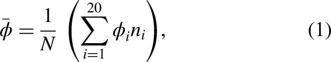

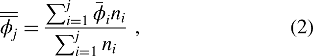
$$\overline{\varphi }={\displaystyle \frac{1}{N}\left(\sum _{i=1}^{20}{\varphi }_i{n}_i\right),}$$

(1)

where $\overline{\varphi }$ is the mean number of phases per possession in a given match, ${\varphi }_i$ is the phase under consideration (from 1 to 20), $n_i$ is the number of possessions that ended in that phase, and N is the total number of possessions in that match. We can compute the running mean of the number of phases per possession in every match played up to a given match as

$$\overline{\overline{{\varphi }_j}}={\displaystyle \frac{{\sum }_{i=1}^j{\overline{\varphi }}_i{n}_i}{{\sum }_{i=1}^j{n}_i},}$$

(2)

where $\overline{\overline{{\varphi }_j}}$ is the running mean following the $j\mathrm{th}$ match, ${\overline{\varphi }}_i$ is the average number of phases per possession in the $i\mathrm{th}$ match, and $n_i$ is the number of possessions observed in the $i\mathrm{th}$ match (details of these calculations are omitted for brevity). These results are shown in Table 6.

Table 6.

The mean number of phases per possession in each match and the running mean of the number of phases per possession as the competition progresses.

Match #	N	Mean Phases	Running Mean
1	79	3.87	3.87
2	93	2.97	3.38
3	105	2.62	3.09
4	122	2.16	2.81
5	119	2.18	2.66
6	93	2.68	2.67
7	106	2.82	2.69
8	103	2.81	2.70
9	85	2.96	2.73
10	103	2.68	2.72
11	90	3.33	2.77
12	118	2.33	2.73
13	92	2.73	2.73
14	96	2.72	2.73
15	91	2.86	2.74

Notes: “Match #” is the match number listed in Table 1. “N” is the total number of possessions in each match. “Mean Phases” is the mean number of phases per possession in each match. “Running Mean” is the weighted average number of phases per possession observed from all of the matches played once each match is completed.

The mean number of phases per possession from every match ranged from 2.16 to 3.87. Table 6 and Figure 2 show that the running mean converges to a reasonably consistent value of approximately 2.73 or 2.74 as the number of games played increases. This result is consistent with the central limit theorem. The grand mean approaches the final value fairly quickly, reaching a value of 2.66 in about five matches (about 500 possessions) and a value of 2.73 in nine matches (about 900 possessions). In the additional six matches the grand mean remains quite steady around the final value with only one excursion following match number 11 between Wales and Scotland (where, as seen in Table 1, an unusually large number of higher phase endings were encountered) that was quickly returned to near the grand mean value by the 12th match between England and Italy (where only a single possession ending beyond seventh phase).

Figure 2.

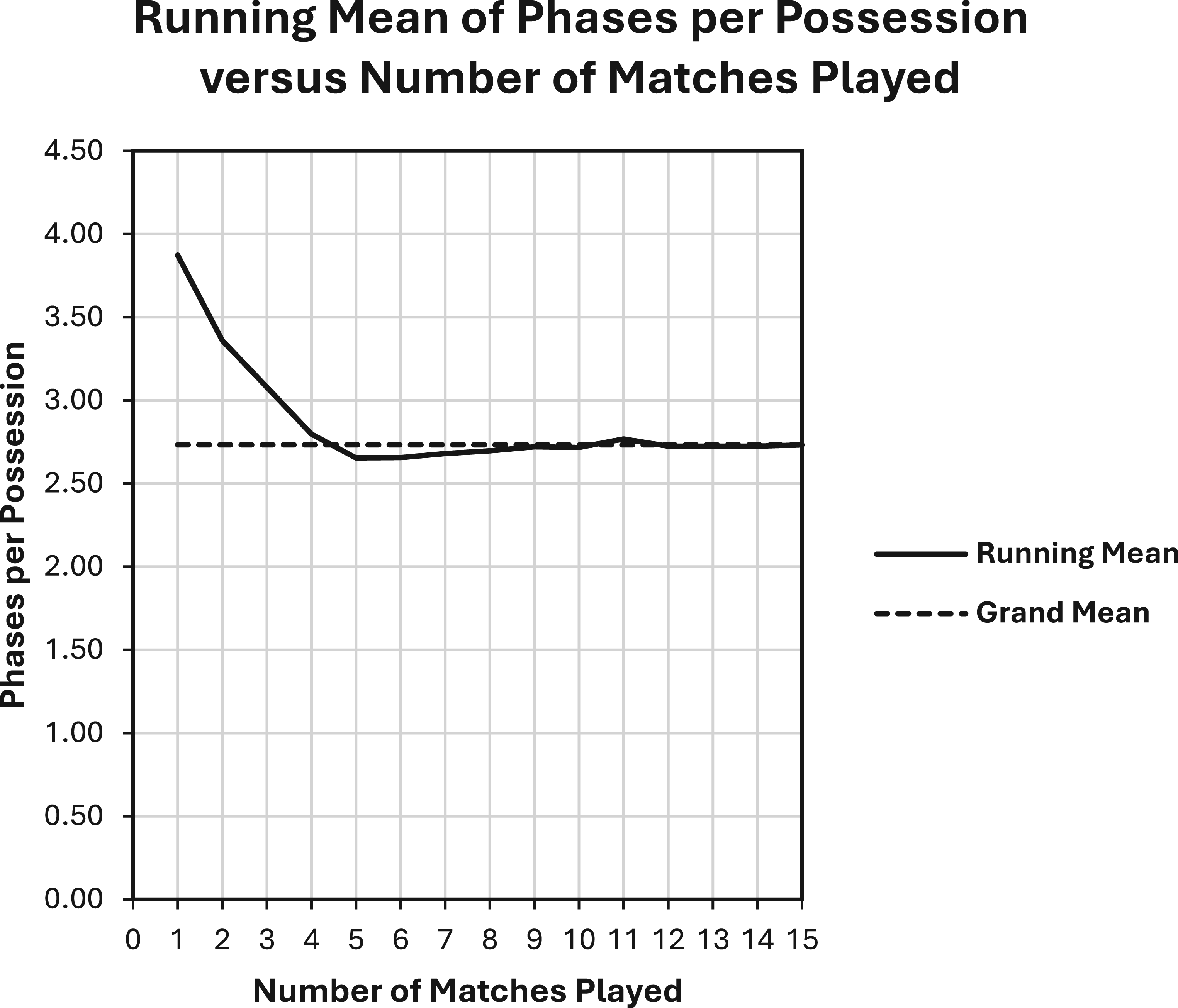
Frequency plot of the running mean of the number of phases per possession as the competition continues. “Running Mean” is the weighted average value of the number of phases per possession observed in all matches up to through the number of matches played. “Grand Mean” is the average number of phases per possession observed through all 1495 possessions observed in the 15 games in the competition (equal to 2.74 phases per possession).

In the parlance of dynamic system (Hiver, 2014), this value of 2.74 is acting as an “attractor state” for the grand mean as the competition continues. Hiver defines an attractor state as a “critical value, pattern, solution, or outcome towards which a system settles down or approaches over time” (p. 21). Dynamic systems do not accidentally end-up at attractor states. The phenomenon is assumed to be the result of self-organization of the system variables and components as the system evolves (p. 22). Self-organization can result without any conscious effort on the part of the agents involved. Under the central limit theorem, the grand mean of the overall distribution is independent of the teams involved or their opponents, is set by the distribution of the overall process, and attracts the mean of a large sample simply as a predictable result of random sampling. This means that the grand mean of the number of phases per possession is fixed a priori and ultimately independent of player or of team approaches to the game. Each match may produce a different mean number of phases per possession, and a team may adapt their play based upon a given tactical situation or a given opponent, but in the aggregate the differences are small and tend to cancel out. Table 6 and Figure 2 both show that the attraction towards the grand mean value is quite strong. This behavior suggests that a reasonable approximation to the overall distribution can likely be achieved by analyzing a smaller subsample of, say, five to nine randomly selected matches rather than all 15. This may provide guidance to investigators of other competitions in estimating appropriate sample sizes for their studies.

The next step in the analysis of this problem is to compare the predicted probability values of the phases in which possession ended derived from various models against the observed values to identify potential generative models. We choose to model the data using two distributions – the geometric distribution and the closely-related discrete Weibull distribution – as potential candidates. Each is defined and described below.

The geometric distribution

Webb (2023) describes the geometric distribution as a discrete distribution that describes the probability of a series of outcomes when there are only two alternatives to each trial. The geometric distribution results from any random experiment that meets all of the following requirements:

The trials are repeated until the desired outcome – often termed the “success” – is achieved.

The trials are independent – that is each outcome is in no way influenced by any previous or future outcome.

There are only two possible outcomes, such as yes or no, heads or tails, six or not six, etc.

The probability of the “success” occurring remains constant in all trials.

The random variable in the distribution includes the number of failures plus the one success in each trial.

In this study “success” is defined as the ending of a possession and the random variable is the phase in which possession ended through any action.

We can estimate the value of the probability of “success” in item four, above, for the geometric distribution from the inverse of the grand mean number of phases per possession value computed for the entire data set (Webb, 2023). As the grand mean was 2.74 phases, our estimate of p for the 2025 Men's Six Nations becomes 0.365.

If we assume that the probability of possession ending in any phase of the distribution is given by p and the probability of possession not ending in any previous phase is given by q (equal to $1-p$ ), the geometric distribution provides the probability mass function (PMF) that the probability that a possession will end in a given phase and can be written as (Webb, 2023)

$$p_{\varphi }=p{q}^{(\varphi -1)},$$

(3)

where ϕ is the phase in which possession ended. A summary table of the observed values of $p_{\varphi }$ and the expected values under the geometric distribution model (and the discrete Weibull distribution, explained below) are shown in Table 7 along with the coefficient of determination ( $r^2$ ) between the data and the various models. The geometric model explains 0.976 (or 97.6%) of the variation in the observed data leaving approximately 2.4% unexplained. A comparison between the aggregated data from Table 1 and the geometric distribution is shown in Figure 3.

Figure 3.

Frequency plot of the probability mass function of the observed probability of possession ending for the data and the geometric distribution versus the phase in which possession ended for the 2025 Men's Six Nations. The probability of possession ending in any phase is 0.365. The coefficient of determination between the data and the geometric model is 0.976.

Table 7.

Table of the probabilities of the phases in which possession ended for the data and two potential models.

Phase	Data	Geometric	Weibull
1	0.415	0.365	0.421
2	0.195	0.232	0.207
3	0.167	0.147	0.125
4	0.067	0.093	0.080
5	0.045	0.059	0.052
6	0.031	0.038	0.035
7	0.026	0.024	0.024
8	0.014	0.015	0.016
9	0.011	0.010	0.011
10	0.009	0.006	0.008
11	0.003	0.004	0.006
12	0.006	0.002	0.004
13	0.004	0.002	0.003
14	0.001	0.001	0.002
15	0.003	0.001	0.001
16	0.000	0.000	0.001
17	0.001	0.000	0.001
18	0.001	0.000	0.001
19	0.000	0.000	0.000
20	0.000	0.000	0.000
r 2	–	0.976	0.989

Notes: “Geometric” is the geometric distribution model with p = 0.365. “Weibull” is the discrete Weibull distribution with α = 0.8563 and β = 2.0281. “r²” is coefficient of determination between the data and the various models. See text for description and details.

Inspection of Table 7 and Figure 3 suggests that the geometric model using p equal to 0.365 provides a reasonable first approximation to the data. Systematic differences between the two do exist however. With the exception of first and third phase endings, the geometric model tends to overestimate the observed data out to around sixth phase endings and tends to underestimate the data for the ninth through 18th phases. In other words, the data tend towards zero more rapidly than the geometric distribution at lower phases and less rapidly as the number of phases increases. The fact that the geometric model underestimates the data at higher phases shows that the data tend to be fat-tailed (Taleb, 2022). This allows a few possession endings to occur occasionally at very high phase count (such as Ireland's 45 phases in 2015) not expected under the geometric model. Note that the probability of the first phase endings (which is, as shown by equation (3) and is always equal to the value of $p$ ) predicted by the geometric model (0.365 or 546 possessions) underestimates the observed probability (0.415 or 620 possessions) by a considerable amount (74 possessions, or an average of approximately 5 possessions per match). Under the geometric model, therefore, we would infer that there is an excess of first phase endings than is predicted by the model. If the geometric distribution were determined to be a valid representation of the data, this observation could be attributable to kicking away more first phase ball than would be expected in a geometric distribution. In the fourth, fifth, and sixth phases, there is a tendency towards too few endings of possessions than are predicted by the geometric model, perhaps attributable to a tendency to play more conservatively than would be expected under the geometric model and, perhaps, illustrates an attempt to play through the phases rather than to concede early possession endings.

A Chi Square Goodness of Fit Test was performed on the fit between the geometric model and the observed data, and is summarized in Table 8. The results indicate that the geometric distribution does not provide a statistically significant representation of the data ( ${\chi }^2(10,N=1,495)=66.40,$ $p<0.001$ ). Examining the contribution of each phase value or range to the total Chi Square shows that the geometric model fails to represent the first five phases well (these five chi square values contribute almost 60% of the total observed Chi Square) and it fails to represent the fat tail area where the phase was greater than or equal to 10 (this represents more than one-third of the total observed Chi Square) – accounting for only 25.1 of the 44 observations in the tail area of 10 phases or greater. The systematic deviations of the data from the geometric distribution quantified here disqualify the geometric distribution as an adequate model of the data.

Table 8.

Chi square goodness of fit test between the observed data and the geometric distribution model.

Geometric Model:
Phases	Count	Geometric	Contrib. to chi sq.
1	620	545.68	10.12
2	291	346.50	8.89
3	250	220.03	4.08
4	100	139.72	11.29
5	67	88.72	5.32
6	47	56.34	1.55
7	39	35.77	0.29
8	21	22.72	0.13
9	16	14.43	0.17
10	14	9.16	2.56
11	5	5.82	0.11
≥12	25	10.12	21.88
Total =	1495	1495.00
Observed Chi Squared =			66.40
df = 12 − 2 =			10
Chi Square crit. =			18.31
p =			<0.001

Notes: “Phases” are the phase categories in which possession ended. “Count” is the number of counts observed in the data for each phase category derived from Table 1. “Geometric” is the expected number of counts computed from the geometric distribution based upon the data. “contrib. to chi sq.” is the contribution to the total observed chi square value for each phase category. “df” is the number of degrees of freedom for this analysis, computed as the total number of phase categories minus 2 (one for requiring the geometric distribution to sum to 1492 and one for the estimation of the value of p (or equivalently, of q)). The analysis reveals that the fit between the data and the geometric model is not statistically significant. In particular, the geometric distribution does an especially poor job of modeling both the data in the earliest phases of play and in the fat tail of the data distribution.

The Poisson Limit Test (described above) was applied to the geometric distribution constructed from the observed number of phases per possession. The results of this test are shown in Table 9. The observed data were found to occur outside of the approximate 95% confidence interval around the geometric distribution in a total of four phases, sometimes exceeding and sometimes being less than the Poisson Limit (the deviant phases are shown in bold italic font in the Table). All four of these exceedances occur in the first five phases. Since the number of observed deviations exceeds the critical value of one deviant value, we conclude that the geometric distribution calculated from the number of phases per possession is not congruent with the data and that the geometric does not provide a statistically significant description of the data.

Table 9.

Poisson limit test applied to the geometric distribution.

			Poisson Trial Limits:
Phase	Data	Geometric	Upper	Lower
1	620	546	592	500
2	291	347	384	310
3	250	220	251	190
4	100	140	164	116
5	67	89	110	71
6	47	56	72	41
7	39	36	49	25
8	21	23	35	14
9	16	14	23	9
10	14	9	17	4
11	5	6	11	2
12	9	4	10	1
13	6	2	7	0
14	2	1	6	0
15	4	1	6	0
16	1	1	6	0
17	1	0	4	0
18	2	0	4	0
19	0	0	4	0
20	0	0	4	0
Total	1495	1495

Notes: “Phase” is the phase in which possession ended. “Data” is the counts of phase endings for all 1495 possessions shown in Table 1. “Geometric” is the number of expected observations in the geometric distribution computed from Table 5 and rounded to nearest integer value. “Poisson Trial Limits” is the approximate 95% confidence interval on the Geometric distribution for each phase (see text for sources). “Upper” is the upper count limit on the confidence interval rounded to the next larger integer value. “Lower” is the lower count limit truncated to the integer value. Data that fall outside of the approximate 95% confidence interval are shown in bold italic font. The data deviated from the geometric distribution in four phases.

In summary, the geometric distribution exhibits systematic departures from the data. Despite the large value of the coefficient of determination for the geometric model, it does not provide an acceptable approximation to the distribution of the observed data.

The discrete Weibull distribution

The Weibull distribution is similar to the geometric distribution but provides an improved alternative in one important aspect – whereas the geometric distribution requires the inflexible assignment of a single value of p throughout its application, the Weibull distribution allows for changes in the probability of the ending of possession in any given phase. This change in probability is limited to a consistent monotonic increase or decrease in the probability through the phases. The discrete Weibull distribution has greater flexibility than the geometric distribution and is also able to model a true geometric distribution as a special case where the probability is held constant through the phases.

The PMF for the discrete Weibull distribution can be determined by a more indirect route than for the geometric distribution (Nakagawa and Osaki, 1975). We first define the cumulative probability of the data from equation (2) as

$$F_{\varphi }=\sum _{i=1}^{\varphi }{p}_i.$$

(4)

where $\varphi$ is the phase in which possession ended. This is the probability of occurrence of a phase less than or equal to given phase $\varphi$ . We then define the exceedance probability as

$$E_{\varphi }=(1-F_{\varphi }).$$

(5)

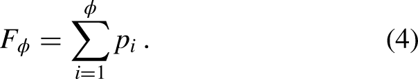
In lifetime studies, this is also referred-to as the survival function and in reliability engineering as the reliability function (Rinne, 2009: 28). This is the probability of occurrence of all phases greater than that of a given phase $\varphi$ .

The exceedance probability by phase for the data computed from equations (4) and (5) is shown as Figure 4. We define the fictitious “zeroeth phase” – it is not possible to have a probability of possession ending in a phase less than one – as having a cumulative probability of zero and an exceedance probability of 1.000. The shape of the curve is similar to the that of the geometric PMF shown in Figure 3 shifted to the right and is, as determined from theory, an exponentially decreasing function (O’Connor and Kleyner, 2012: 37).

Figure 4.

Frequency plot of the exceedance probability of the phases in which possession ended in the 2025 Men's Six Nations derived from the observed data.

A next step in determining the PMF of the discrete Weibull distribution is to use the exceedance probability and the phase number to create a Weibull plot (Rinne, 2009: 45; Jones, 2019: 201). Theoretical considerations provide the equation for calculating the exceedance probability from basic parameters. This is given (Jones, 2019: 203) as:

$$E_{\varphi }=(1-F_{\varphi })=e^{{(-\varphi /\beta )}^{\alpha }},$$

(6)

where $\varphi$ is the phase and $\alpha$ and $\beta$ are the Weibull distribution shape parameter and scale parameter, respectively. Taking the natural logarithm of both sides yields

$$Ln(E_{\varphi })=-{\left({\displaystyle \frac{\varphi }{\beta }}\right)}^{\alpha }.$$

(7)

Changing signs and taking the natural logarithm of both sides again leads to

$$Ln(-Ln(E_{\varphi }))=\alpha Ln(\varphi )-\alpha Ln(\beta ).$$

(8)

This is the equation of a straight line in the form of y = mx + b, with slope m equal to α and β equal to

$$\beta =e^{(|b|/\alpha )}$$

(9)

where, in this case, $|b|$ is the absolute value of the intercept. The Weibull plot is constructed by graphing $Ln(-Ln(E_{\varphi }))$ versus $Ln(\varphi )$ and is shown in Figure 5. The equation of the best-fit line on the plot is given by the equation $Ln(-Ln(E_{\varphi }))=0.8563(Ln(\varphi ))-0.6055$ . The agreement is strikingly linear over nearly three log-cycles. From this, the value of α is 0.856 and β is computed from equation (9) as 2.028. The coefficient of determination between the data and the line is 0.998, indicating that only 0.2% of the variation in the transformed data is not explained by the Weibull plot.

Figure 5.

Weibull Plot for the 2025 Men's Six Nations. The equation of the least squares fit to the data is Ln(−Ln(Exceedance)) = 0.8563(Ln(ϕ)) − 0.6055. The coefficient of determination for this plot is 0.998. The value of α computed for this distribution is 0.8563. The value of β is 2.0281.

Based upon the values of α and β we can compute the value of the best fit estimate the value of $q_w$ as (O’Connor and Kleyner, 2012: 37)

$$q_w=exp\left[-{\left({\displaystyle \frac{1}{\beta }}\right)}^{\alpha }\right],$$

(10)

or $q_w=0.579$ . Using this value of $q_w$ we compute the exceedance probability of the discrete Weibull distribution for each phase (calculation omitted for brevity) as (Nakagawa and Osaki, 1975):

$$E_{\varphi }=(q_w^{\varphi }{)}^{\alpha }.$$

(11)

The exceedance probability computed from this equation is essentially coincident with the plot of the observed data in Figure 4 and is not depicted separately.

The PMF for the discrete Weibull distribution may be calculated from differencing the exceedance probability (Nakagawa and Osaki, 1975) of equation (11) as

$$p_{\varphi }=E_{\varphi }-E_{(\varphi +1)}=(q_w^{\varphi }{)}^{\alpha }-(q_w^{(\varphi +1)}{)}^{\alpha }.$$

(12)

The PMF for the discrete Weibull model are given in Table 7 and shown along with the data in Figure 6. The discrete Weibull distribution tracks the data well at both the lowest and highest phases without the systematic deviations observed in the geometric distribution (Figure 3). We note that the probability of possession ending in the first phase predicted by the discrete Weibull model (0.421) is quite similar to that in the data (0.415). Under the discrete Weibull model, this observation tends to disconfirm and eliminate any necessary hypothesis of kicking away too much possession in first phase. If the discrete Weibull model adequately explains the data, it is not surprising that teams would have deduced through time the appropriate maximum entropy number of first phase endings. The coefficient of determination between the data and discrete Weibull model is 0.989 leaving only 0.011 – or approximately one percent – to unexplained variation.

Figure 6.

Frequency plot of the probability mass function of the observed probability of possession ending for the data and the discrete Weibull distributions versus the phase in which possession ended for the 2025 Men's Six Nations. The α-value for the discrete Weibull distribution is 0.8563. The β-value is 2.0281. The coefficient of determination between the data and the discrete Weibull distribution is 0.989.

A Chi Square Goodness of Fit Test was performed on the fit between the discrete Weibull model and the observed data, and is summarized in Table 10. As with the Chi Square Test on the geometric distribution, the results indicate that the discrete Weibull distribution does not provide a statistically significant representation of the data ( ${\chi }^2(10,N=1,495)=32.08,p<0.001$ ). Unlike the geometric model, however, the discrete Weibull model differs greatly from the data only in the number of third phase endings. The observed contribution of the third phase endings to the total observed Chi Square (23.32) is more than 66% of the total. The discrete Weibull model captures the fat-tailed distribution of the data well, accounting for 43.3 of the 44 observed values in phases greater than or equal to 10. While this test rejects the discrete Weibull distribution as a significant match to the data distribution, the fact that there is only one phase that accounts for the majority of the excess Chi Square raises the suspicion that only this phase may be truly deviant from the model (as stated before, real data are never actually distributed according to any known distribution (Conover, 1999; 454)). If there is a logical reason that explains this single deviation from the discrete Weibull distribution, it would be reasonable to assume that the data are, in general, well represented by the discrete Weibull distribution, but that some additional phenomenon may be at play in third phase. We suggest, below, just such a phenomenon to explain this deviation.

Table 10.

Chi square goodness of fit test between the observed data and the discrete Weibull distribution model.

Discrete Weibull Model:
Phases	Count	Weibull	Contrib. to chi sq.
1	620	629.40	0.14
2	291	309.47	1.10
3	250	186.88	21.32
4	100	119.60	3.21
5	67	77.74	1.48
6	47	52.33	0.54
7	39	35.88	0.27
8	21	23.92	0.36
9	16	16.45	0.01
10	14	11.96	0.35
11	5	8.97	1.76
12	9	5.98	1.53
≥13	16	16.42	0.01
Total =	1495	1495.00
		Observed Chi Squared =	32.08
		df = 13 − 3 =	10
		Chi Square crit. =	18.31
		p =	<0.001

Notes: “Phases” are the phase categories in which possession ended. “Count” is the number of counts observed in the data for each phase category derived from Table 1. “Weibull” is the expected number of counts computed from the discrete Weibull distribution based upon the data. “contrib. to chi sq.” is the contribution to the total observed chi square value for each phase category. “df” is the number of degrees of freedom for this analysis, computed as the total number of phase categories minus 3 (one for requiring the discrete Weibull distribution to sum to 1492 and one each for the estimation of the values of α and β). The analysis reveals that the fit between the data and the discrete Weibull model is not statistically significant due primarily to the excessive number counts of third phase endings.

The results of the values of α and β from this analysis can be interpreted in rugby terms. The value of the Weibull shape parameter α is less than unity. When this occurs, it indicates that the probability of a possession ending in a given phase decreases as the phases increase (Jones, 2019: 203). In other words, as play continues it becomes less and less likely that the possession will end in the current phase. This effect can be quantified through computing the probability of possession ending given the phase of possession. This is termed the hazard rate or failure rate in reliability engineering (Rinne, 2009: 120) and is given by

$$h_{\varphi }={\displaystyle \frac{(E_{(\varphi -1)}-E_{\varphi })}{E_{(\varphi -1)}},}$$

(13)

with $E_0$ equal to one. The value of $h_{\varphi }$ is computed from the discrete Weibull distribution (results of this calculation are omitted for brevity). This value can be defined (Rinne, 2009: 28) in rugby terms as the approximate probability that possession will be ended immediately (i.e., – in the next phase of play) given that possession has not ended up to that time. This value can be interpreted as a true probability. Figure 7 shows the probability of possession ending in any given phase of play for the data in this study. The initial probability is approximately 0.42 and decreases smoothly to approximately 0.27 at the 20th phase. It is, therefore, roughly two-thirds as likely for possession to end in the 20th phase than in the first phase. This phenomenon results in the observed fat-tailed distribution of the data.

Figure 7.

Frequency plot of the probability of possession ending given the phase of possession derived from the discrete Weibull distribution. The probability of possession ending decreases as the number of phases increases as a power law as predicted for a discrete Weibull model.

Evidence that the value of $h_{\varphi }$ changes (in this case, decreases) monotonically as the phases increase is, we believe, a novel observation not previously described in the rugby literature. In a sense, this validates the concept of playing through the phases in that the attacking team is more likely to retain possession as the phases increase. As the defense struggles to maintain its shape, a talented attack may expose more opportunities to score points. Playing through the phases does not guarantee success, but it may improve the odds over other alternatives.

This result is reasonable in rugby terms. Initially, the defense might be well-organized and difficult to break through. Possession may end intentionally through the attack choosing to kick ahead or accidentally by committing an infraction, but it is more likely that a handling attack will occur, a tackle will be made, and play will progress to the next phase. As the number of phases increase the defense is likely to become less organized (a la Biscombe and Drewett, 1998) and may be less likely to compete aggressively for the ball. The defenders are content to make tackles and prepare for the next phase of their defense. The attackers are less prone to probing the defense and are more focused on retaining possession. Play becomes longitudinally static, characterized by defenders not committing many players to the ruck and attackers moving from ruck to ruck laterally across the field. This phenomenon is often observed late in matches as player fatigue sets-in. As play progresses the attackers rack-up additional phases. When this happens it is also relatively unlikely that possession will end in any given phase absent an attacking handling error, foul play detected by the Referee, a kick attempting to break the stalemate, or the scoring of points through a try or a dropped goal. Aggressive and efficient play in the early phases may give way to more desultory efforts. The probability of possession ending in the next phase initially drops rapidly and then less rapidly at higher phases.

Turning attention to the value of β, this scaling parameter is also termed the characteristic life (Jones, 2019: 202) of the Weibull distribution, a measure of the spread of the PMF. Smaller values of β limit the number of observations at larger values. It is always equal to the abscissa value where the cumulative probability is equal to 0.6321 (Rinne, 2009: 337) or the exceedance probability of 0.3679 (see Figure 4). The value of β should therefore be somewhat smaller than the mean number of phases per possession. The value of β was observed to be equal to 2.028 which, indeed, is somewhat less than the mean number of phases per possession of 2.74. If β were larger we would expect to see many more possessions ending beyond 10 (or so) phases.

The Poisson Limit Test was applied to the discrete Weibull distribution constructed from the estimated values of $\alpha$ and $\beta$ derived from the observed data. The result of this test are shown in Table 11. The observed data were found to occur outside of the approximate 95% confidence interval around the discrete Weibull distribution only once, in third phase. Since the number of observed deviations does not exceed the critical value of one, we conclude that the discrete Weibull model is congruent with the data.

Table 11.

Poisson limit test applied to the discrete Weibull distribution.

			Poisson Trial Limits:
Phase	Data	Weibull	Upper	Lower
1	620	627	677	577
2	291	309	344	274
3	250	187	215	160
4	100	120	143	99
5	67	79	98	62
6	47	53	69	39
7	39	36	49	25
8	21	25	37	16
9	16	17	27	9
10	14	12	21	6
11	5	9	17	4
12	9	6	13	2
13	6	4	10	1
14	2	3	9	1
15	4	2	7	0
16	1	2	7	0
17	1	1	6	0
18	2	1	6	0
19	0	1	6	0
20	0	0	4	0
> 21	0	1	6	0
Total	1495	1495

Notes: “Phase” is the phase in which possession ended. Note that a category of “≥21” phases was added to accommodate the final expected discrete Weibull count. “Data” is the counts of phase endings for all 1495 possessions shown in Table 1. “Weibull” is the number of expected observations in the discrete Weibull distribution computed from Table 5 and rounded to nearest integer value. “Poisson Trial Limits” is the approximate 95% confidence interval on the discrete Weibull distribution for each phase (see text for sources). “Upper” is the upper count limit on the confidence interval rounded to the next largest integer value. “Lower” is the lower count limit truncated to the integer value. Data that fall outside of the approximate 95% confidence interval are shown in bold italic font. The data deviated from the discrete Weibull distribution in only one phase.

This Poisson Limit Test result coupled with the large value of the coefficient of determination for the model suggests that the discrete Weibull distribution provides a reasonable approximation to the distribution of the observed data despite failing the Chi Square Goodness of Fit Test. We conclude that the data are better represented by the discrete Weibull distribution computed with parameters determined from the data rather than the geometric distribution determined from the mean number of phases per possession.

Summary of the analyses

Analysis of the distribution of the phases in which possession ended in the 2025 Men's Six Nations has resulted in several interesting results. The aggregated data tend to follow rather approximately the geometric distribution. This is, we believe, that first time in the literature that the phases of possession have been shown to have a reasonably predictable mathematical relationship (at the distribution level) between the count/proportion of phase endings and the phase number. A mathematical relationship suggests a degree of predictability. While the end of possession is well-described by the occurrence of a seemingly random event, the processes involved in producing the observed distributional patterns of the phases in which possession ended constrain the solution and result in the observed distribution.

A second summary point is that the data have identifiable systematic deviations from the geometric. The geometric distribution approximation to the observed data does not pass the Chi Square Goodness of Fit Test, due to these systematic differences.

This deviation is corrected in large measure by applying the discrete Weibull distribution to the data. While the discrete Weibull distribution also fails to pass the Chi Square Goodness of Fit Test, the failure is due almost exclusively to an excessive number of third phase endings observed beyond the number predicted. Otherwise, the fit between the data and the discrete Weibull distribution is quite acceptable. Despite the negative result of the Chi Square Goodness of Fit Test, the discrete Weibull model, combined with a rationale for the excessive number of third phase endings (see below), provides a reasonable description of the data. The discrete Weibull distribution allows for the observed probability of possession ending decreasing as the phases increase. This observation is also novel, is documented in Figure 7, and accounts for the observed fat-tailed distribution in the data. It also successfully explains the occasional observation of possession ending in extremely high phase numbers than would be expected in a geometric distribution.

The data exhibit a statistically significant deviation from the discrete Weibull distribution only in the third phase. Review of all of the match videos in the data collection process revealed a strikingly frequent adherence by all teams to a specific strategy following receiving a kick in a less-advantageous field position (often inside their 22-meter line and near the touchline). Typically, a player receiving the kick under pressure from the defense is immediately tackled (end of the first phase of possession). The team then passes the ball to forward runners a bit farther away from the touchline. The ball is recycled from the tackle (end of the second phase) creating some space on the weak side of play and the ball is cleared upfield or to touch via a kick (ending the possession in third phase). The observed deviation in third phase likely results from the occurrence of this consistently executed tactical ploy executed by all teams in the competition.

Quantitatively, the data show 250 third phase endings. The discrete Weibull model and the Poisson Limit Test on that model (Table 11) indicate that 187 third phase endings would be expected to occur and that 215 third phase endings would have been the greatest number expected given the Poisson trial upper limit on third phase endings. This accounts for a difference of 63 third phase endings from the number observed and a total of 35 excess third phase endings throughout the competition. These imply an average of 4.2 more third phase endings than expected per match and, importantly, an average excess of 2.3 third phase endings beyond the upper Poisson limit per match.

When an event is premeditated – that it is a planned response to a common and recurring tactical situation – the assumption of every phase ending occurring randomly is violated. It is reasonable to assume that the a priori decision to kick on many of the third phases artificially inflates the number of third phase endings and will impact, to some degree, the probabilities of possession endings in adjacent phases. This is perhaps evident in the third phase endings for all teams depicted in Figures 1 and 6. We should expect a lack of absolute model agreement with the data as the occurrence of a planned solution to this specific tactical situation is far from random.

While not seeming to be a large number of excess events out of a total of 100 possessions per match, a few excess third phase endings in each match appears sufficient to create a significant difference between the data and the discrete Weibull model. While consistent actions characteristic of only one specific team would likely get lost in the aggregation, even a minor tendency occurring outside of the expected distribution exhibited by many teams will be observable over a large number of matches. In fact, modeling the distribution may be the best way to detect significant impacts of any such subtle tendency.

Accepting that the probability of the phases in which possession ends are generally described by a discrete Weibull distribution has several important implications. The first is that the observed decrease in the probability of possession ending in a given phase as the phases increase in the 2025 Men's Six Nations must be taken to be a feature rather than an accident. Whether or not the proposed mechanism of this decrease is precisely as hypothesized in the text, we must acknowledge that the change is real and needs to be accepted as fact. Additional research will show whether this effect is consistent across other competitions, age-grades, and gender.

Second, Rinne (2009: 19) argues that the failures that give rise to the discrete Weibull distribution often result from an underlying degradation process. Operation of a system can be affected by both wear-and-tear through time and by the occurrence of randomly distributed shocks to the system. The system fails either when wear-and-tear accumulates beyond an acceptable safe level or a fatal shock occurs. Biscombe & Drewett's (1998) description of attackers disfiguring the defense as play progresses through the phases may represent the wear-and-tear on the defensive system in which the players suffer from increasing fatigue and resultant minor errors in their play.

Shocks induce additional stress on the system when they occur. The shocks could result from occasional significant errors on the part of defenders and the scoring of points, from errors on the part of the attack such as knock-ons or penalties, or from decisions on the part of the Referee. Any of these could happen in any phase of any possession and, therefore, should be randomly distributed. Random shocks could also be precipitated by an unexpectedly powerful or innovative thrust by the attack (or by the defense). Individual shocks may not be sufficient to cause an end of possession by themselves, but given the magnitude of any error or attacking thrust and the field position where it occurs, a shock – by itself or in conjunction with accumulated wear-and-tear – could well determine whether the possession ends in that phase or not. The geometric distribution does not explicitly consider the wear-and-tear aspect of the discrete Weibull distribution in its assumption that the probability of ending a possession in any given phase is constant.

Given the joint wear-and-tear and random shock explanations, a third implication of the discrete Weibull distribution is that it should be possible to apply coaching interventions to improve the performance of the system. Both processes could be improved through player conditioning and through thoughtful player substitution. Wear-and-tear could be mitigated through improved fitness and injury treatment or by player substitution approaches. Random shocks could be administered in attack through different attacking patterns, improved player strength and power, and by the use of impact players. Defensive shocks might involve developing and implementing more effective and efficient systems, through tactical ploys such as targeting the ball in tackles, and through improved counter-rucking. Enterprising coaches should always be seeking these results.

Successful changes in approach and tactics are likely to result in different overall phase ending distributions as they are adopted by the other competitors. We expect that innovations have occurred through time and have changed the overall distribution as effective novel approaches propagate through the teams in the competition. Historical data on the phases in which possession ended in previous competitions might be reviewed profitably in this light.

Finally, it is unlikely that the hypothesized overall distribution and the attractor towards the mean number of phases per possession of 2.74 were developed according to any person's whim. As in any self-organizing system, it is far more likely that the inherent variability in the playing of rugby has been constrained by other limits – including the Laws of Game, how the Referees interpret and apply those Laws, and coaching approaches and innovations – resulting in the observed aggregated distribution of phases in which possession ended. As such, it is also unlikely to be very easy to manipulate changes in the overall distribution absent implementation of changes in the Law, interpretations, or coaching approaches adopted by multiple competitors in a competition unless an innovative solution is shown to produce a marked improvement in team performance. Then the change would propagate through the competition and result in a new stable equilibrium in the distributions.

Conclusions

The results of this study have led to several observations that contribute to our understanding of the game of rugby. Analysis of the data from the 2025 Men's Six Nations revealed that the count of possessions obtained by each team in the six matches was not significantly different from a Gaussian (and in accordance with a Poisson model with a large mean value). The median value in the sample was 50 and the mean value was nearly the same. It is reasonable to conclude, therefore, that we can expect approximately 50 possessions per team performance or about 100 possessions per match in similar competitions. Additionally, the average number of phases in each of the 1495 possessions was strongly attracted to the value of 2.74, resulting in most possessions ending in relatively few possessions. It is unusual to reach more than 10 phases in a given possession. These values place limits on the expected number of tackles and rucks expected in a match and on the finite number of scoring opportunities available to the teams.

The distribution of the probability of possession ending in a particular phase (Table 1) shows that the greatest number of possession endings occurred in the first phase of play (41.5%) and decreased more-or-less smoothly as the number of phases increased. The shape is reminiscent of an exponential or, in this case as the data are discrete, a geometric (or similar) distribution.

Analysis revealed that the geometric distribution provides a close first approximation to the data. This is the first time this result has appeared in the literature. A possible fit of the geometric distribution to the data is accomplished using a value of p equal to 0.365 (Figure 3). The coefficient of determination computed between the PMF of the data and the geometric model (Table 7) was 0.976 – almost 98% of the variation in the data is explained by this geometric distribution. While this is a considerable amount, important systematic differences exist between the geometric model and the data. These differences show that, in general, phase values below about five phases the geometric model tends to overpredict the probability of occurrence and beyond five phases it tends to underpredict the probability. The geometric model does not pass the Chi Square Goodness of Fit Test due to these systematic differences between the geometric and the data distributions – the data are not congruent with a geometric distribution. This is confirmed by the results of the Poisson Limit Test where the observed number of possession endings fall outside of the approximate 95% confidence limits on the model in four occasions rather than the maximum expected number of one (Table 9). We must conclude that the geometric model, despite its high overall coefficient of determination, does not adequately describe the data.

The PMF of the data was also compared to the discrete Weibull distribution (Table 7 and Figure 6) computed from the data. This distribution is more flexible than the geometric in that the probability of possession ending in any given phase can vary consistently through the observations. Visually, this model compares well to the data with no obvious systematic variations. The coefficient of determination using the discrete Weibull model increased from 0.978 for the geometric model to 0.989 for the discrete Weibull model (Table 7). The unexplained variation is only about 1%. While the discrete Weibull model does not pass the Chi Square Goodness of Fit Test, a deeper look into the contribution to the total observed Chi Square reveals that the reason for the failure was solely due to the excessive number of third phases endings. Further, the Poisson Limit test shows that the data deviate from the approximate 95% confidence limit in only that one phase (Table 11). Successfully describing many aspects of the distribution of the number of phases per possession in rugby as a discrete Weibull distribution is a major finding of this study.

The discrete Weibull probability of possession ending in the next phase of play is seen to decrease as the phases increase (Figure 7). The ending of a possession in the highest phase observed is approximately only two-thirds as probable as an ending in the possession in the first phase, and this decrease in possession endings as the phase increases leads to the observed fat-tail in the data. The values of the two Weibull parameters (Figure 5) of α – the shape parameter equal to 0.856 – and β – the scale parameter or characteristic life (Rinne, 2009, p. 32) of the Weibull distribution equal to 2.028 – have reasonable rugby interpretations consistent with the observed data. The shape parameter α is less than one – giving rise to the decrease in the probability that possession will be lost in the next phase as the phases increase – and the value of β is slightly less than the mean number of phases per possession (the theoretical value of β occurs at the 36.8th percentile of the exceedance probability curve).

The observation that this effect results in the probability of losing possession decreases as the phases of play increase is a novel one not previously reported in the literature. By itself this explains the fat-tailed distribution of the phases in which possession ended. It suggests that playing through the phases while maintaining heavy attacking pressure provides more attacking opportunities and could be a favored approach in terms of rugby success.

We conclude that the data from the sample of the 2025 Men's Six Nations distribution of the phase in which possession ended is congruent with the discrete Weibull distribution with parameters derived from the data modified by the observation of excessive third phase endings. Further research is needed to test the hypothesis whether the discrete Weibull model of the data from the phases in which possession ends might hold in other competitions, at different age-grades, and in the women's game. This seems likely, however, based upon the fact that the game is played under essentially the same Laws in all competitions and at all levels. Any differences might demonstrate effects of other coaching approaches or player talent on the playing of the game.

Stepping back a bit from mathematical and statistical rigor, it may be best to consider the following as an explanation of the observed PMF of the data. To a first approximation, the data are fairly well-described by a geometric model (r² = 0.976) where there is an intrinsic probability that possession will end in any given phase – suggesting that the phase in which possession ends is in large measure random. Superimposed on this are two additional factors resulting from consideration of the discrete Weibull distribution as a better model. The first is caused by changes in the probability that possession will be lost in any given phase shown by the value of α of less than one. This factor then accounts for an additional 0.013 to the coefficient of determination (r² = 0.989) in the discrete Weibull model, and explains the fat-tail observed in the data. The second factor involves the over-representation of third phase endings in the data relative to the discrete Weibull distribution. This may be due to a common pattern of play in modern rugby. Additional research is necessary to test whether the result of this investigation apply universally among all competitions beyond the 2025 Men's Six Nation.