Sage Journals: Discover world-class research

Abstract

In the literature, information on the rally length distribution is quite incomplete, fragmented and non-homogeneous. In this paper we fill the gap deeply analyzing the distribution of rally length in professional tennis matches in the following directions: i) we provide the empirical distribution of the rally length, not only for some categories, but for each single length; ii) we consider different distributions for men and women and for different surfaces; iii) we find the statistical distribution best fitting the data for each surface; iv) we show how the rally distribution depends on some variables, such as the probabilities of winning a point at serve and players’ heights; v) previous points are based on a much larger sample size than other works leading to very reliable results. Our analyses point out that the best distribution for rally length is a zero-one-modified Geometric distribution, whose parameters are functions of the probabilities of winning a point at serve and of the players’ heights. Results suggest that the the players’ heights is the most impacting variable on the rally length distribution.

Keywords

Rally length distribution height of players Quasi-Poisson models zero-one-modified geometric distribution zero-one-modified Poisson distribution

1 Introduction

A rally in tennis is the sequence of back and forth shots between players, within a single point. A rally starts with the serve, can involve any kind of shot and ends when a point is scored.

Rally statistics, particularly rally lengths, are useful to measure different styles of play, to define strategies of play and to analyze different aspects of the game (Makino et al., 2020). Usually players dominant on serve tend to play shorter rallies while baseliner players are often engaged in significantly longer rallies. As the majority of points are 4 shots or fewer, some analysts have stressed the importance of a game strategy designed to close the point as fast as possible.

Besides the style of play, the rally length is affected by several other factors: obviously, by the game context but also by the court surface, by balls features, by weather conditions and by the physical characteristics and gender of players. Slower surfaces, as clay courts, tend to produce longer rallies than hard and, even more, grass courts. Hotter weather fosters faster balls, helping the servers and, potentially, increasing the 0–4 rally count. Likewise, taller players tend to be associated to shorter rallies due to their strong service.

For all these reasons, the number of shots in a point, i.e. the rally length, can and should be treated as a random variable. As a consequence, we can wonder which is the distribution of such a random variable. Although this issue is very interesting, it has received relatively little attention in the literature and, to date, only very partial and incomplete results are available. In the present work, we fill the gap on the rally length distribution deeply analyzing it and improving the existing literature in several directions: i) we provide the distribution of rally length for men and women, and for each surface, not limited to the first 10–15 shots, as often done, but for any observed rally length. This allows to appreciate the frequency of quite long rallies; ii) our analyses are based on a very large sample size, around 500, 000 points for men and around 250, 000 points for women. This is by far the largest number of points considered in literature. As a consequence, results should be very stable also for not too short rally lengths; iii) separately for men and women and for each surface, we look for the best statistical distribution for the rally length, in particular we consider the quasi-Poisson distribution, the Geometric distribution and two of their variants, namely the zero-modified Poisson/Geometric distributions and the zero-one-modified Poisson/Geometric distribution, specifically built to produce more accurate estimates of the zero and one rally frequencies; iv) for the same distributions we consider time-varying parameter versions, where parameters depend on other exogenous variables. This, in turn, allows us to study which variables significantly impact on the rally length. An interesting result is that players’ height is particularly relevant for the rally length distribution. To the best of our knowledge, this kind of study is new and has never been done before. While many studies assessed the importance of players’ heights to explain the serve strength (Vaverka and Cernosek, 2013; Pascual, 2023), to predict match outcomes (Bieniek and Kwater, 2015; Gao and Kowalczyk, 2021) or within the betting context (Candila and Palazzo, 2020), none has connected the height with rally lengths.

In our analysis, we focus on parametric distributions, mainly because it is much more complex to generate data from a nonparametric distribution, while anyone can easily generate data from a parametric distribution as soon as (estimated) parameters are known. A parametric distribution is particularly useful when the rally length is used in a simulation context, as in Kovalchik and Ingram (2018) or in Lisi and Grigoletto (2021), who used it to simulate the duration of professional tennis matches. In addition, the parametric approach allows a comparison in terms of parameters’ values and is less sensitive to the presence of several zero frequencies, as observed in the empirical distribution.

The rest of the paper is organized as follows. In Section 2 the literature on rally length distributions is reviewed. In Section 3 we introduce the dataset and provide descriptive analyses. Section 4 is devoted to describe some probabilistic models for the rally length. Estimation results are discussed in Section 5 while the comparison among competitor models is performed in Section 6. Section 7 concludes.

2 Literature review

In the current literature, information on rally length distribution is quite incomplete, fragmented and non-homogeneous.

Fernandez-Fernandez et al. (2008) analyzed eight well-trained female tennis players, 6 of which were ranked between 300 and 800 in the Women’s Tennis Association (WTA) singles ranking (one player was the current European Junior Champion) and, for outdoor clay-court surface, reported a mean rally length of 2.5 ± 1.6 shots per rally.

In a four-set Davis Cup match, used as a case study, Gomes et al. (2011) found that the number of strokes per rally decreases during the match.

Carboch et al. (2019) analyzed the rally pace characteristics and the frequency of rally shots in 7 male (1738 points) and 23 female (2926 points) matches at the Australian Open 2017 and provided a graphical representation of the distribution of rally length for men and for women up to 20+ shots 1 . They found that the frequency of rally shots was similar for the two genders. In the whole match, the rally finished within the first four shots in 59% (men) and in 62% (women) of cases; within 5–8 shots in 27% (men) and 27% (women) of cases; 9 and more shots were required in 14% (men) and 11% (women) of cases.

In a paper focusing on how the use of new balls affects the match characteristics and the frequency of rally shots Carboch et al. (2020) provided observed frequencies of rally length up to 13 shots. However, their results are based on a limited number of matches: 23 female matches played at the Australian Open (1141 points) and 24 male matches played at the Australian Open (699 points), French Open (838 points) and Wimbledon (537 points) in 2017.

Mlakara and Kovalchik (2020) provided a graphical representation of the rally length based on 66 male matches (8026 points) and 64 female matches (4834 points) played during the 2017 Australian Open tournament. However, since they were interested in analyzing time pressure rallies, they included only points longer than 2 shots.

In a study aimed at establishing the prevalence and importance of individual rally lengths within points of 0, 1, 2, 3 and 4 shots in terms of winning elite grass court tennis matches, Fitzpatrick et al. (2021) considered data from 211 male and 209 male Wimbledon singles matches between 2015 and 2017. Their results revealed an underlying prevalence of short points (compared to medium length and long points) on grass courts for both genders, with 66% (for women) and 72% (for men) of all points played at Wimbledon between 2015 and 2017 ending in fewer than 5 shots. Based on the considered data, they also provided the mean percentage of points played per match of 0, 1, 2, 3 and 4 shot rally lengths, both for men and for women.

In his blog, Ingram (2021) studied how the average rally length by surface changed over time in male tennis and showed that, from 1970 to 2020, the average length tended to become more homogeneous across surfaces.

On the website tennisabstract.com, the Match Charting Project provides the average rally length for a number of players, as well as statistics for rally length classified within the categories 1 - 3 shots, 4 - 6 shots, 7 - 9 shots and 10+ shots. Other websites show classifications based on slightly different categories. Further pieces of information about rally length frequencies can be found in specialized websites, as Stat on the T (on-the-t.com) which gives the frequency of rallies longer than four shots for several professional players or the server win percentage by rally length.

To determine a reasonable distribution of the shots per point Kovalchik and Ingram (2018) examined the relationship between the number of shots per rally and the service bonus and malus 2 and the surface of the match using data from 1582 male matches and 966 female matches. They suggested that the expected shot count and variance could be accurately approximated with a quasi-Poisson distribution conditional on the service bonus. This is the only work which attempted to pinpoint a statistical distribution for the rally length, even if the authors didn’t give any detail on how they found it.

3 The dataset

The dataset on which the analyses are performed is based on data available on the Match Charting Project (MCP), a crowdsourced effort to track shot-by-shot data in professional tennis, created by Jeff Sackman and available on Github 3 . However, the rally length of each point is not directly available, but has been extrapolated by the information included in the dataset, using an ad hoc code written in R language. In this way we were able to obtain the rally lengths for 5751 male and 3413 female professional matches since year 2000. This permitted us to analyze the rally lengths of 503, 946 points played in the male circuit and 247, 392 points played in the female circuit. A detailed description of the sample sizes for different surfaces and gender, is given in Table 1. These numbers are sensibly higher than those considered in the works quoted in the introduction. This very large sample size is important in order to have a good estimate of occurrences of low-frequency rally lengths and should ensure a good reliability of our analyses for each single surface.

Table 1
Matches and points sample sizes for men and women and for different surfaces

Men Women

Surface N. of matches N. of points N. of matches N. of points

Grass 710 70,333 912 65,705

Hard 3,332 290,340 1,833 130,235

Clay 1,709 142,253 686 51,449

Total 5,751 503,946 3,431 247,389

	Men	Women
Grass	710	70,333	912	65,705
Hard	3,332	290,340	1,833	130,235
Clay	1,709	142,253	686	51,449
Total	5,751	503,946	3,431	247,389

Note that, being MCP a crowdsourced project,it does not contain all the matches played in a given period.

3.1 Descriptive analyses

The definition of rally length is not uniform across literature and blogs, depending on whether serve counts as a shot or not. In this work we use the definition given in the MCP: the serve counts as a shot, but errors do not. Thus, a double fault is 0 shots, and an ace or unreturned serve is 1. A rally with a serve, three additional shots and an error on an attempted fifth shot counts as 4.

Figure 1 shows the empirical rally distribution for men on each surface up to 25 shots. The absolute frequencies for the whole distribution are listed in Table 14 of the Appendix 4 , while Table 2 provides some descriptive statistics.

Fig. 1

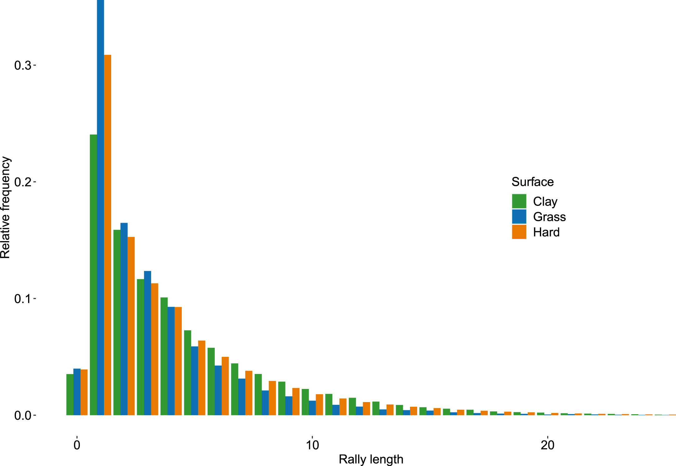
Men: Rally distribution for the first 20 shots for clay, hard and grass surfaces.

Table 2

Men: Descriptive statistics for rally distribution for each surface. SD=standard deviation; S=Skewness coefficient; K=Kurtosis coefficient; q_α=α-th quantile

Surface	Mean	SD	Mode	S	K	q _2,5	q ₅	q ₁₀	q ₂₅	q ₅₀	q ₇₅	q ₉₀	q ₉₅	q _97,5	Max
Grass	3.2	3.1	1	2.1	8.6	0	1	1	1	2	4	7	10	12	48
Hard	3.8	3.8	1	1.9	7.4	0	1	1	1	2	5	9	12	15	59
Clay	4.3	4.1	1	1.8	7.0	0	1	1	1	3	6	10	13	15	83

Double faults occur around 3.5% of times on clay and around 3.9% of times on hard surfaces and grass, highlighting that, on the whole, there is no surface strategy involving double faults apart from, maybe, taking a little greater risk on grass and hard surfaces. The largest differences among surfaces come in the case of just one shot, which occurs in 24.0% of cases on clay, in 30.9% of cases on hard surfaces and in 35.6% of times on grass. For number of shots greater than one differences are less pronounced. For rally lengths greater than four the observed frequency on grass is always smaller than for clay and hard surfaces. This confirms that, on grass, players try to close the point faster. On the contrary, starting from four shots, the higher frequencies are those related to clay. For all surfaces the rally length’s mode is 1 while the median is 3 on clay and 2 for grass and hard. It is also interesting to note that rallies lasting more that 15 shots occur in 2.6% of times on clay, 2.3% of times on hard and only 1.1% of times on grass. Although low, these frequencies are not completely negligible, as assumed by several categorizations. In our dataset, for men, the largest rally values are 83 for clay, 59 for hard 5 and 48 for grass.

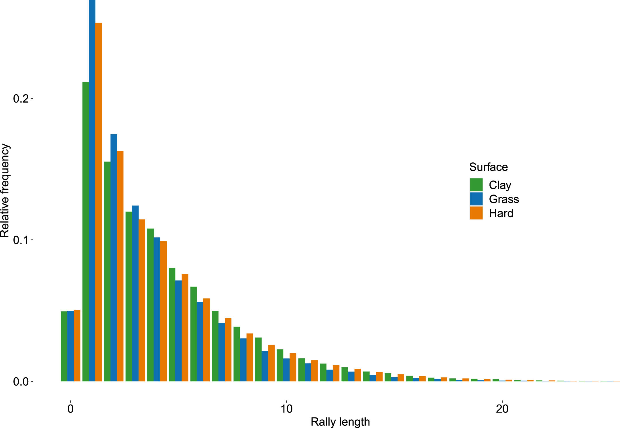
Analogously, Fig. 2 shows the rally distribution for women on each surface up to 25 shots. Table 2 gives some descriptive statistics for the whole distribution, whose absolute frequencies are listed in Table 15 of the Appendix.

Fig. 2

Women: Rally distribution for the first 20 shots for clay, hard and grass surfaces.

In female matches, double faults occur around 5.0% of times independently of the surface, a little more often than for men. Even if the summary descriptive statistics are quite similar to those for men, the histogram in Fig. 2 globally shows less pronounced differences among surfaces with respect to men. Also, very long rallies are less frequent than in male matches: for instance, rallies long at least 18 shots occur 0.5% of times on hard, 0.27% of times on grass and 0.65% of times on clay for women, against the corresponding 1.1%, 0.5% and 1.2% for men. In our female dataset, the longest rallies lengths are 48 on hard courts and clay and 34 on grass.

It is however curious that the longest rally in professional tennis was played by two women. During the 1984 Virginia Slims tournament, the tennis players Vicki Nelson and Jean Hepner played a point hitting 643 shots over 29 minutes.

Table 3

Women: Descriptive statistics for rally distribution for each surface. SD=standard deviation; S=Skewness coefficient; K=Kurtosis coefficient; q_α=α-th quantile

Surface	Mean	SD	Mode	S	K	q _2,5	q ₅	q ₁₀	q ₂₅	q ₅₀	q ₇₅	q ₉₀	q ₉₅	q _97,5	Max
Grass	3.5	3.1	1	1.5	5.5	0	1	1	1	3	5	8	10	12	34
Hard	3.9	3.5	1	1.6	5.8	0	0	1	1	3	5	9	11	13	48
Clay	4.2	3.6	1	1.6	6.4	0	1	1	1	3	6	9	12	14	48

4 Probabilistic models

Using the previously described dataset, this section aims at finding probabilistic models able to suitably represent the rally length distribution on different surfaces, both for male and female professional players. Note that, while some authors consider only strictly positive rally lengths (Kovalchik and Ingram, 2018), in this work we try to model the whole distribution, including the case of 0 length, i.e. double faults.

This is a challenging task, since empirical rally length distributions exhibit over-dispersion as well as less zero observations and more one observations than would be allowed, for example, by the Poisson model. The same issues arise when adapting a Geometric distribution.

This critical point requires, hence, to devote specific attention to zero and one frequencies. The need to modify a discrete distribution in order to better model the count of zeros is often encountered in the literature. Zero-inflated (Lambert, 1992) and hurdle models (Mullahy, 1986; Heilbron, 1994) were proposed to improve the fitting of e.g. Poisson, Geometric or negative binomial count models which, in their regular versions, were unable to yield realistic zero counts. Likewise, the literature contains analyses in which discrete distributions are modified for both zero and one counts (Qi et al., 2019; Mohammadi et al., 2021). Below, when using these kinds of distributions, we will refer to them as zero-modified or zero-one-modified. Most properties of a zero-(one-) modified distribution follow easily from its unmodified counterpart.

In the next two subsections, first we consider unconditional models which try to adapt some known distribution to the data. In particular, we consider the quasi-Poisson distribution and the zero-modified versions of the Poisson and Geometric models, to account for deflated zeros. Moreover, to improve the fitting, for both distributions we propose further variants that we call zero-one-modified. The zero-one-modified Poisson distribution and the zero-one-modified Geometric distribution are built to jointly account for deflated zeros and inflated ones values. In all these cases, the goal is to estimate the models’ parameters, assumed to be constant, and to find the distribution which best fits the data.

Secondly, in order to further improve the fitting, for the quasi-Poisson model, the zero-one-modified Poisson and the zero-one-modified Geometric distributions, parameters are allowed to depend on some exogenous variables. This permits also to analyze which variables significantly affect the rally length.

4.1 Unconditional models

Since rally lengths are count data taking discrete, non negative values occurring independently, we may think of modeling them by means of a Poisson distribution or a Geometric distribution.

However, in a Poisson distribution mean and variance coincide. In our case, instead, this assumption is clearly violated: for instance, for the male matches on hard surfaces, the rally’s mean is 3.8 while, due to a very long right tail, the rally’s variance is 14.56, and similar results also hold on grass and clay.

A possible solution to handle the over-dispersion is to refer to the quasi-Poisson model. This is a model, for a variable Y, assumes that E (Y) = λ and Var (Y) = φ · λ, where the dispersion parameter φ is unrestricted and is estimated from the data. The quasi-Poisson model is not a distribution but, rather, a model belonging to the family of generalized linear models (see Nelder and Wedderburn, 1972 and McCullagh and Nelder, 1989) with link function defined as

$log (λ) = β_{0} + β_{1} X_{1} + β_{2} X_{2} + . . . + β_{q} X_{q},$ (1) where λ is the mean of the response variable, and X₁, …, X_q are suitable regressors. The unconditional version of model (1) has no explanatory variables and, thus, $\hat{λ} = exp ({\hat{β}}_{0})$ .

To face zero-deflation and one-inflation, we estimate zero-modified and zero-one-modified Poisson and Geometric distributions.

In detail, the zero-modified Poisson (zmPois) distribution is a discrete mixture between a degenerate distribution at zero and a standard Poisson. If Y ∼ zmPois (p₀, λ) its probability mass function is given by:

$P (Y = y) = {\begin{matrix} p (0) = p_{0} \\ p (y) = \frac{1 - p_{0}}{1 - e^{- λ}} f (y) y = 1, 2, . . . \end{matrix}$ (2) with λ > 0, 0 ≤ p₀ ≤ 1 and f (y) being the probability mass function of a Poisson distribution with parameter λ.

The probability mass function of a r.v. Y having zero-modified Geometric (zmGeom) distribution, Y ∼ zmGeom (p₀, p), is given by

$P (Y = y) = {\begin{matrix} p (0) = p_{0} \\ p (y) = \frac{1 - p_{0}}{(1 - p)} f (y) y = 1, 2, . . . \end{matrix}$ (3) with 0 ≤ p₀ ≤ 1, 0 < p < 1 and f (y) being the probability mass function of a Geometric distribution with parameter p.

Generalizing the zero-modified distributions we obtain the zero-one-modified distributions, which are discrete mixtures between two degenerate distributions at zero and one and a standard distribution f (y). For example, the probability mass function of a r.v. Y having zero-one-modified Poisson (zomPois) distribution, Y ∼ zomPois (p₀, p₁, λ) is given by

$\begin{matrix} P (Y = y) \\ = {\begin{matrix} p (0) = p_{0} \\ p (1) = p_{1} \\ p (y) = \frac{1 - p_{0} - p_{1}}{1 - e^{- λ} (1 + λ)} f (y) y = 2, 3, . . . \end{matrix} \end{matrix}$ (4) with 0 ≤ p₀ ≤ 1, 0 ≤ p₁ ≤ 1, 0 < p < 1 and f (y) being the probability mass function of a Poisson distribution with parameter λ.

Likewise, if Y is a zero-one-modified Geometric (zomGeom) distribution, Y ∼ zomGeom (p₀, p₁, p) its distribution is

$P (Y = y) = {\begin{matrix} p (0) = p_{0} \\ p (1) = p_{1} \\ p (y) = \frac{1 - p_{0} - p_{1}}{(1 - p)^{2}} f (y) y = 2, 3, . . . \end{matrix}$ (5) with 0 ≤ p₀ ≤ 1, 0 ≤ p₁ ≤ 1, 0 < p < 1 and f (y) being the probability mass function of the Geometric distribution with parameter p.

Parameters p₀, p₁, p and λ (depending on which distribution is used) can be estimated by maximum likelihood.

4.2 Conditional models

To improve the distribution’s fitting, and in agreement with the approach followed by Kovalchik and Ingram (2018), in this section we allow the distribution’s parameters to be non-constant across the matches. To achieve this goal, we write the distribution’s parameters as a function of some variables describing the matches’ features which, possibly, affect the rally length.

As the quasi-Poisson model belongs to the GLM family, representing the dependence of parameter λ on some exogenous variables is quite straightforward and consists in including the regressors in equation (1). For instance, Kovalchik and Ingram (2018) considered a quasi-Poisson model where λ was written as a function of just one variable X denoting the sum of the probabilities of each two player to win the point at serve. In particular, for their data, they found $\hat{λ} = 2.89 - 1 \cdot X$ and $\hat{φ} = 3.3$ , for men, and $\hat{λ} = 2.33 - 0.7 \cdot X$ and $\hat{φ} = 2.7$ , for women.

For the zero-one modified Geometric and Poisson distributions we allow p (0), the probability of zero length rallies, i.e. of double faults, to depend on the surface but not on other variables. The reason is our assumption that, on average, players try to minimize the number of double faults in any situation, but they may accept to take some risk on surfaces rewarding good serves.

For the zomPois and zomGeom models, we make parameters match-dependent by writing them as functions of exogenous variables. In the case of the the zomGeom model, and for the i-th point, as parameters p_1,i and p_i, which represent probabilities, we write their logit transformation as a linear function of q regressors:

$\begin{matrix} log (\frac{p_{1, i}}{1 - p_{1, i}}) = \sum_{j = 0}^{q} γ_{j} X_{i, j} and \\ log (\frac{p_{i}}{1 - p_{i}}) = \sum_{j = 0}^{q} β_{j} X_{i, j} \end{matrix}$ (6) with X_i,0 = 1, so that for the i-th point we can write

$\begin{matrix} p_{1, i} = \frac{exp (\sum_{j = 0}^{q} γ_{j} X_{i, j})}{1 + exp (\sum_{j = 0}^{q} γ_{j} X_{i, j})} and \\ p_{i} = \frac{exp (\sum_{j = 0}^{q} β_{j} X_{i, j})}{1 + exp (\sum_{j = 0}^{q} β_{j} X_{i, j})} \end{matrix}$ (7) where γ_j and β_j, j = 0, 1, . . . , q are unknown parameters to be estimated and X₁, …, X_q are known explanatory variables. This representation assures that p_1,i and p_i belong to the (0, 1) interval.

When considering a zomPois model, parameter p_1,i has the same representation while, since λ_i must be positive, we write

$λ_{i} = exp (\sum_{j = 0}^{q} δ_{j} X_{i, j})$ (8) where δ_j, j = 0, 1, . . . , q, are parameters to be estimated.

In this paper, all parameters are estimated by maximum likelihood.

5 Estimation results

In this section the previously described models are applied to our dataset. For each surface and for both genders, they consist of the sequence y_i, i = 1, . . . , N, of rally lengths, where i is the point considered.

The set of explanatory variables X_j,i considered in this work is:

- X₁ = P_a + P_b, where P_x is the probability that player x wins the point at serve;

- X₂ = |P_a - P_b|;

- X₃ = log(H_a + H_b), where H_x is the height of player x in cm;

- X₄ = |H_a - H_b|.

In addition, as we consider different models for each surface, estimated parameters also implicitly depend on this variable. The first two variables X₁ and X₂ were used also by Kovalchik and Ingram (2018), while the (log) sum and the absolute difference of heights have never been considered before. The absolute difference and the sum of the probabilities of winning the point at serve are often used to describe the difference in quality and the overall quality of two players. Intuitively, one can expect that the higher the overall quality the longer the rallies because neither of the two players dominates the other one. On the contrary, the higher the difference in quality the shorter the rallies because the stronger player should manage to quickly win the point. Of course, all these considerations hold on average. The rationale behind the consideration of the players’ height as a driver for rally lengths is that a strong serve can make a player have an upper hand after the serve, thus having the opportunity to close up the point. In turn, the service strength is favoured by the player’s height as witnessed by the fact that great servers are usually quite tall players (Bieniek and Kwater, 2015).

Thus, the (absolute) difference in the players’ heights may impact on rally lengths, especially on a fast surface. However, the heights’ difference says nothing about the actual players’ heights and this motivate the consideration also of the sum of the players’ heights. As concerns the use of the logarithm of the heights sum, it is just due to a better fit of models to data with respect to the simple sum 6 . Note that even if X₃ and X₄ are related to the players’ height, there are not collinearity issues because the two transformations make them not very correlated: for men their correlation is 0.295 while for women it is only 0.102.

Actually, we also considered the sum and the absolute difference of ATP/WTA ranking but they never resulted significant. In this work P_a and P_b are the fractions of points won at serve by each player in the match within which the i-th point was played. This explains the large variability of X₁ and X₂ as shown in Table 4, which displays some descriptive statistics for these four variables in our dataset.

Table 4
Statistical features of regressor variables. They were computed over the whole dataset, without distinction on surface

Variables Min. Q(0.05) Q(0.25) Median Q(0.75) Q(0.95) Max

X ₁ 0.727 0.971 1.121 1.206 1.288 1.407 1.670

X ₂ 0.001 0.028 0.112 0.194 0.280 0.399 0.693

exp (X₃) 348 365 372 374 378 390 411

X ₄ 0 0 0 2 7 15 41

Variables	Min.	Q(0.05)	Q(0.25)	Median	Q(0.75)	Q(0.95)	Max
X ₁	0.727	0.971	1.121	1.206	1.288	1.407	1.670
X ₂	0.001	0.028	0.112	0.194	0.280	0.399	0.693
exp (X₃)	348	365	372	374	378	390	411
X ₄	0	0	0	2	7	15	41

The estimated parameters and related p-values for quasi-Poisson conditional models, for men, are listed in Table 5, for two different specifications: the one suggested by Kovalchik and Ingram (2018), including only X₁ = P_a + P_b and denoted by QP_KI, and the specification including all the X variables, denoted by QP. The estimates of the same parameters for women are listed in Table 6.

Table 5

Men: Estimated parameters and, between parentheses, the corresponding p-value for conditional quasi-Poisson models. QP_KI denotes the Kovalchik and Ingram (2018) specification

	Grass		Hard		Clay
Variables	QP	QP_KI	QP	QP_KI	QP	QP_KI
β₀	16.806	1.257	13.402	1.531	18.336	1.627
	(<0.001)	(<0.001)	(<0.001)	(<0.001)	(<0.001)	(<0.001)
β₁	0.0032	-0.084	-0.053	-0.157	-0.070	-0.136
	(0.364)	(<0.001)	(<0.001)	(<0.001)	(<0.001)	(<0.001)
β₂	-0.126	–	-0.156	–	-0.123	–
	(0.002)	–	(<0.001)	–	(<0.001)	–
β₃	-2.645	–	-2.017	–	-2.829	–
	(<0.001)	–	(<0.001)	–	(<0.001)	–
β₄	0.003	–	-0.001	–	-0.002	–
	(<0.001)	–	(0.006)	–	(<0.001)	–
φ	3.0	3.0	3.8	3.8	3.8	3.8

Table 6

Women: Estimated parameters and, between parentheses, the corresponding p-value for conditional quasi-Poisson models. QP_KI denotes the Kovalchik and Ingram (2018). specification

	Grass		Hard		Clay
Variables	QP	QP_KI	QP	QP_KI	QP	QP_KI
β₀	29.61	1.400	24.13	1.601	27.19	1.507
	(<0.001)	(<0.001)	(<0.001)	(<0.001)	(<0.001)	(<0.001)
β₁	-0.084	-0.123	-0.130	-0.213	0.156	-0.063
	(0.001)	(<0.001)	(<0.001)	(<0.001)	(0.011)	(0.011)
β₂	0.034	–	-0.070	–	-0.463	–
	(0.263)	–	(0.001)	–	(<0.001)	–
β₃	-4.821	–	-3.86	–	-4.415	–
	(<0.001)	–	(<0.001)	–	(<0.001)	–
β₄	-0.0032	–	0.002	–	-0.003	–
	(0.001)	–	(<0.001)	–	(<0.001)	–
φ	2.7	2.7	3.1	3.2	3.2	3.2

In the QP specification, all four variables are significant, with the exception of X₁ = P_a + P_b for men on grass and of X₂ = |P_a - P_b| for women on grass. This gives a first suggestion of the relevance of the height’s role on the rally length. For QP_KI models, parameters have been re-estimated on our dataset. Both for men and women, while dispersion parameters φ are quite similar to those found by Kovalchik and Ingram (2018), estimated β₁ parameters, defining the linear dependence of λ on P_a + P_b, are sensibly different, even if in agreement with the sign.

Estimation results for zero-one-modified Geometric (zomGeom) and Poisson (zomPois) are listed in Table 7, for men, and in Table 8, for women. As shown in equations (4) and (5), zomPois and zomGeom models have three parameters, i.e. p₀, p₁ and λ the former and p₀, p₁ and p, the latter. Parameter p₀ is assumed constant, while the other ones depend on regressors.

Table 7

Men: Estimated parameters and, between parentheses, corresponding p-value for conditional zero-one-modified Geometric and Poisson models

		Geometric			Poisson
p _i	Param	Grass	Hard	Clay	Grass	Hard	Clay
	γ ₀	-32.47	-33.50	-39.72	-33.01	-33.51	-39.72
		(<0.001)	(<0.001)	(<0.001)	(<0.001)	(<0.001)	(<0.001)
	γ ₁	0.298	0.246	0.140	0.302	0.245	0.140
		(0.005)	(<0.001)	(0.055)	(0.004)	(<0.001)	(0.057)
p ₁	γ ₂	0.115	0.210	0.372	0.110	0.210	0.372
		(0.339)	(<0.001)	(<0.001)	(0.359)	(<0.001)	(<0.001)
	γ ₃	5.31	5.458	6.470	5.405	5.459	6.469
		(<0.001)	(<0.001)	(<0.001)	(<0.001)	(<0.001)	(<0.001)
	γ ₄	-0.004	-0.0001	0.005	-0.004	-0.0001	0.005
		(0.021)	(0.986)	(<0.001)	(<0.017)	(0.982)	(<0.001)
	β₀	-13.51	-8.156	-15.58	11.425	7.43	12.80
		(<0.001)	(<0.001)	(<0.001)	(<0.001)	(<0.001)	(<0.001)
	β₁	-0.123	0.003	0.114	0.091	0.001	-0.080
		(0.108)	(0.923)	(0.006)	(0.008)	(0.912)	(<0.001)
p/λ	β₂	0.138	0.194	0.093	-0.099	-0.139	-0.066
		(0.113)	(<0.001)	(0.055)	(0.010)	(<0.001)	(<0.001)
	β₃	2.136	1.161	2.385	-1.694	-0.969	-1.853
		(<0.001)	(<0.001)	(<0.001)	(<0.001)	(<0.001)	(<0.001)
	β₄	-0.002	0.001	0.003	0.002	0.001	-0.002
		(0.057)	(0.006)	(<0.001)	(<0.001)	(<0.001)	(<0.001)

Table 8

Women: Estimated parameters and, between parentheses, corresponding p-value for conditional zero-one-modified Geometric and Poisson models

		Geometric			Poisson
p _i	param	Grass	Hard	Clay	Grass	Hard	Clay
	γ ₀	-47.86	-35.55	-50.39	-44.06	-37.57	-50.27
		(<0.001)	(<0.001)	(<0.001)	(<0.001)	(<0.001)	(<0.001)
	γ ₁	0.212	0.171	-0.162	0.214	0.180	-0.164
		(0.027)	(0.007)	(0.172)	(0.002)	(0.005)	(0.169)
p ₁	γ ₂	0.039	0.284	0.921	0.045	0.270	0.926
		(0.723)	(<0.001)	(<0.001)	(0.679)	(<0.001)	(<0.00)
	γ ₃	7.950	5.840	8.382	7.302	6.183	8.363
		(<0.001)	(<0.001)	(<0.001)	(<0.001)	(<0.001)	(<0.001)
	γ ₄	0.004	-0.001	0.001	0.005	-0.001	-0.001
		(0.066)	(0.439)	(0.785)	(0.046)	(0.434)	(0.778)
	β₀	-32.00	-25.54	-28.25	25.43	20.23	23.14
		(<0.001)	(<0.001)	(<0.001)	(<0.001)	(<0.001)	(<0.001)
	β₁	0.091	0.158	-0.214	-0.052	-0.112	0.151
		(0.138)	(<0.001)	(0.001)	(0.052)	(<0.001)	(<0.001)
p/λ	β₂	-0.072	0.037	0.470	0.044	-0.024	-0.334
		(0.300)	(0.425)	(<0.001)	(0.144)	(0.201)	(<0.001)
	β₃	5.27	4.129	4.642	4.072	-3.154	-3.687
		(<0.001)	(<0.001)	(<0.001)	(<0.001)	(<0.001)	(<0.001)
	β₄	0.004	-0.001	0.005	-0.003	(0.001)	0.004
		(0.014)	(0.125)	(0.001)	(<0.001)	(0.010)	(<0.001)

Apart for the constant, the only variable which is always significant for all parameters, all models, all surfaces and gender is X₃ = log (H_a + H_b). This is an evidence that the (log) sum of the players’ heights is the most important variable to explain the rally length.

Tables 7 and 8 show the estimation results for the full models but successive analyses have been performed re-estimating the models including only the significant variables. To better appreciate the impact of each (significant) variable on the models’ parameters and, hence, on the probability distribution of the rally length, we can use equations (7) and (8) and observe how p₁, p and λ change as a function of the estimated parameters and of the X variables.

To isolate the effect of a single variable X_j, we fix the values of all other X_i (i ≠ j) to their average within our sample, while letting X_j vary between the sample minimum and maximum. For example, Fig. 3 shows the effect of the regressors on the parameters p₁ and p of a zomGeom for men on grass. For p₁, we can see that the most impacting variable is log (H_a + H_b) (panel in position (1,2)) which causes p₁ to vary from 0.29 to 0.47, with a range of 0.18. Also, P_a + P_b has a significant, although lower, impact leading to a variation of p₁ in a range of 0.08 (panel in position (1,1)). Much less important is the role of the difference between the players’ heights (panel in position (2,1)). Moreover, while increasing log (H_a + H_b) leads to a higher probability of rallies of length 1, the opposite occurs for |H_a - H_b|. Indeed, a large heights’ difference implies that one of the players is quite short and this, often, reduces the serve power and, thus, the probability that the point ends in just one shot. For p the only significant variable is log (H_a + H_b), stressing the importance of the players physical characteristics for the rally length. Figure 3 makes also clear that the heights’ sum has a lower impact on p, which varies in a range of 0.06.

Fig. 3

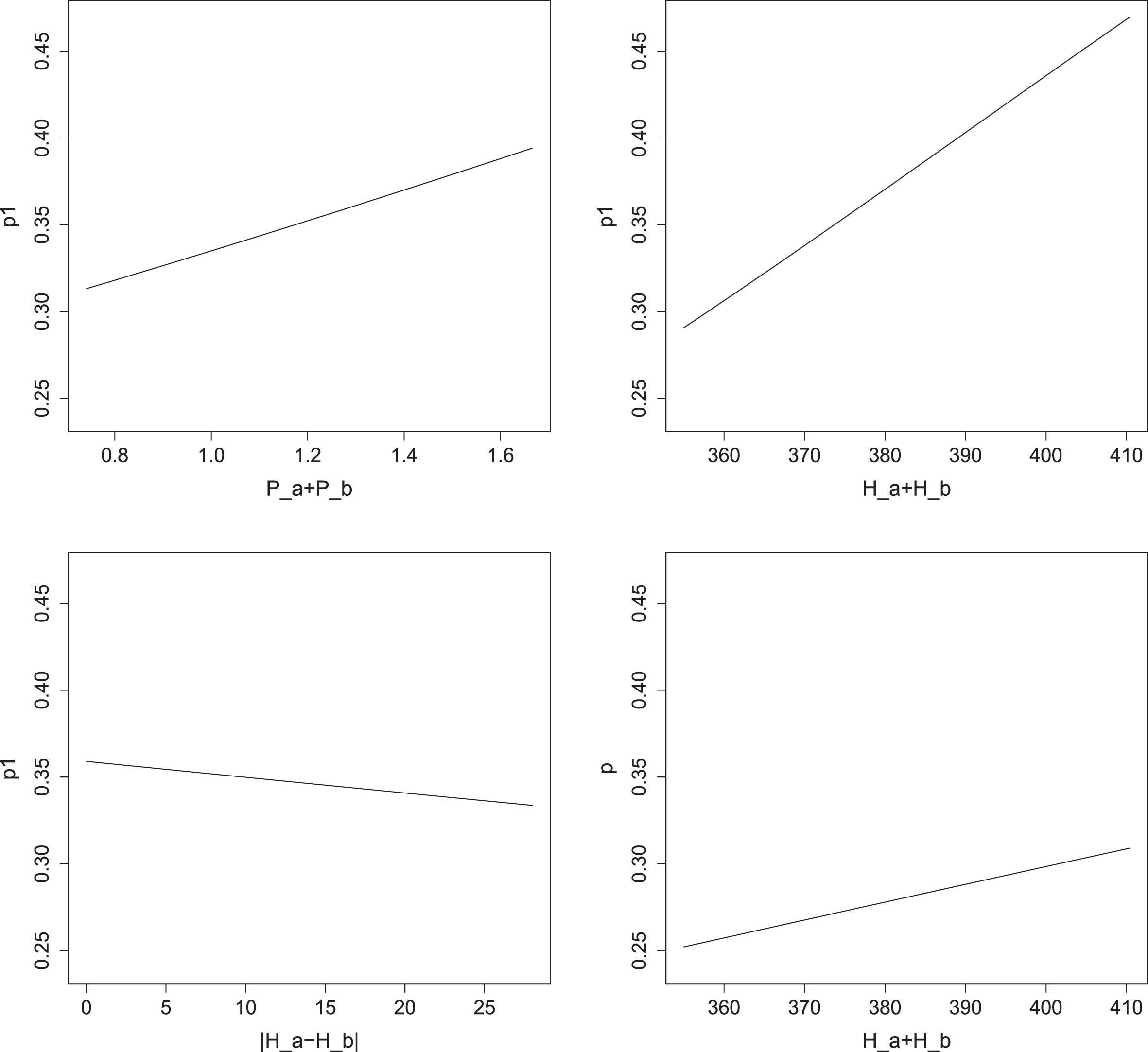
Impact of the significant X_i variables on p₁ and p on grass for men. Panel position (1,1): impact of P_a + P_b on p₁; position (1,2): impact of log (H_a + H_b) on p₁; position (2,1): impact of |H_a - H_b| on p₁; position (2,2): impact of log (H_a + H_b) on p. For a better understanding, the tick labels refer to (H_a + H_b) instead of to log (H_a + H_b).

Figure 4 focuses on the impact of log (H_a + H_b) on p₁ and p across different surfaces. We can see that, for a given sum of heights and average values of the other variables, the estimated distributions lead to the the highest value of p₁ for grass, followed by hard surfaces and by clay. This is not surprising as we know that on fast surfaces rallies of length 1 have higher probability than on slower surfaces. At the same time, we notice that the range of variation of p₁ due to log (H_a + H_b) is constant across surfaces: 0.18 on grass and hard and 0.17 on clay. This witnesses that height is an important factor to define the probability of one-shot rally on all surfaces, even if this probability differs according to the surface.

Fig. 4

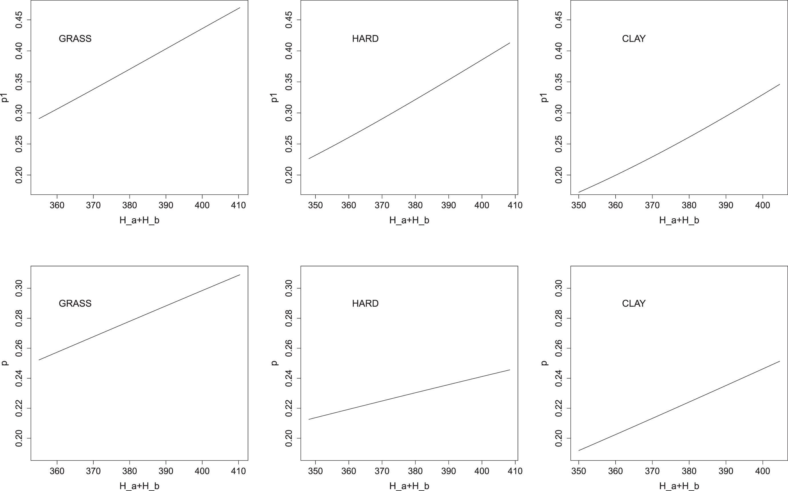
Impact of log (H_a + H_b) on p₁ and p across different surfaces. First column: grass; second column: hard; third column: clay. For a better understanding, the tick labels refer to (H_a + H_b) instead of to log (H_a + H_b).

The impact of log (H_a + H_b) on p is less important but, on grass, this is the only significant variable. Again, the range of variation of p due to log (H_a + H_b) is not very different among surfaces: 0.06, 0.045 and 0.055 on grass, hard and clay, respectively.

Similar considerations also hold for the conditional zom-Poisson but we have focused on the zom-Geometric because in the following section it will result to be best performing one.

6 Comparisons

In this section we evaluate the ability of the estimated distributions to reproduce the observed ones. We compare the performances of the proposed distributions:

i) by summing the absolute differences between observed ( $P_{i}^{obs}$ ) and estimated ( $P_{i}^{est}$ ) probability masses of a rally of length i:

$Δ_{M} = \sum_{i = 0}^{M} | P_{i}^{obs} - P_{i}^{est} |$ (9) where M is the maximum rally length considered.

ii) by applying the Kolmogorov-Smirnov test to asses the equality between the best distributions produced by our models and the empirical distributions.

For a better insight, when computing Δ_M, we consider M = 10, 20 and the maximum observed length on each surface.

Tables 9 (for men) and 10 (for women) list the Δ_M indicators for unconditional models. Both for men and women, it is clear that Geometric models produce sizable better results than Poisson models and that zero-one-modified models produce sensibly better results than zero-modified models with the only exception of clay for women, for which indicators of zmGeom and zomGeom models are quite similar. Within the class of unconditional models, thus, we can doubtless conclude that the zero-one-modified Geometric distribution is the one leading to the best fitting.

Table 9

Unconditional models for men: Values of indicators Δ_M for each surface and for different fittings. QP=Quasi-Poisson, zm=zero modified, zom=zero-one-modified

Men	Grass			Hard			Clay
Distribution	Δ₁₀	Δ₂₀	Δ_all	Δ₁₀	Δ₂₀	Δ_all	Δ₁₀	Δ₂₀	Δ_all
QP	0.543	0.556	0.558	0.500	0.518	0.521	0.487	0.524	0.527
zmPois	0.554	0.601	0.606	0.590	0.663	0.672	0.582	0.666	0.676
zmGeom	0.152	0.162	0.165	0.157	0.168	0.172	0.061	0.067	0.069
zomPois	0.260	0.297	0.301	0.335	0.384	0.393	0.366	0.423	0.433
zomGeom	0.032	0.037	0.039	0.027	0.032	0.034	0.022	0.025	0.026

Table 10

Unconditional models for women: Values of indicators Δ_M on each surface and for different fittings. QP=Quasi-Poisson, zm=zero modified, zom=zero-one-modified

Women	Grass			Hard			Clay
Distribution	Δ₁₀	Δ₂₀	Δ_all	Δ₁₀	Δ₂₀	Δ_all	Δ₁₀	Δ₂₀	Δ_all
QP	0.488	0.542	0.544	0.547	0.616	0.621	0.525	0.599	0.604
zmPois	0.469	0.522	0.524	0.524	0.592	0.597	0.494	0.565	0.570
zmGeom	0.049	0.054	0.055	0.058	0.062	0.063	0.051	0.056	0.059
zomPois	0.262	0.306	0.308	0.300	0.351	0.355	0.306	0.358	0.363
zomGeom	0.022	0.026	0.027	0.023	0.026	0.027	0.049	0.054	0.056

Tables 11 (for men) and 12 (for women) list the values of Δ_M for conditional models. In this case we consider two versions of the quasi Poisson models: one using all regressors and one adopting the Kovalchik and Ingram’s specification, which only considers X₁. For the modified Poisson and Geometric models we list results only for the zero-one-modified versions, as results in Tables 9 and 10 suggest that zero-modified versions produce worse fittings.

Table 11

Conditional models for men: Values of indicators Δ_M on each surface and for different fittings. The letter V in the models’ name denotes varying parameters

Men	Grass			Hard			Clay
Distribution	Δ₁₀	Δ₂₀	Δ_all	Δ₁₀	Δ₂₀	Δ_all	Δ₁₀	Δ₂₀	Δ_all
QP-V	0.360	0.369	0.372	0.319	0.329	0.333	0.246	0.252	0.255
QP_KI-V	0.360	0.369	0.362	0.321	0.330	0.334	0.246	0.252	0.255
zomPois-V	0.248	0.287	0.291	0.249	0.289	0.296	0.361	0.419	0.427
zomGeom-V	0.025	0.031	0.033	0.023	0.028	0.031	0.020	0.024	0.025

Table 12

Conditional models for women: Values of indicators Δ_M on each surface and for different fittings. The letter V in the models’ name denotes varying parameters

Women	Grass			Hard			Clay
Distribution	Δ₁₀	Δ₂₀	Δ_all	Δ₁₀	Δ₂₀	Δ_all	Δ₁₀	Δ₂₀	Δ_all
QP-V	0.243	0.252	0.253	0.232	0.238	0.240	0.168	0.173	0.174
QP_KI-V	0.245	0.253	0.255	0.230	0.237	0.239	0.173	0.177	0.179
zomPois-V	0.250	0.294	0.296	0.289	0.342	0.346	0.368	0.418	0.423
zomGeom-V	0.033	0.038	0.039	0.026	0.031	0.032	0.051	0.057	0.059

In general, and in terms of Δ_M, conditional models provide better results than unconditional ones except in the case of zomGeom for women, for which the unconditional model provides slightly better results. The two versions of quasi-Poisson models show a strong reduction of Δ_M and provide extremely similar results. For men, however, their performance is worse than for both zomPois and zomGeom models. Differently, for women, they show values of Δ_M lower than those of the zomPois model. As for unconditional models, the zomGeom models is clearly the best one. For men, the conditional zomGeom models lead to an improvement ranging from 10% to 28% in terms of Δ₁₀, with respect to the unconditional zomGeom models.

To assess the statistical equality between the model-implied distributions and the empirical ones, we now apply the well-known Kolmogorov-Smirnov test for goodness-of-fit. The test is applied to the distributions produced by the conditional zero-one-modified models, which are those leading to the best fit in terms of Δ_M.

To be independent of the specific sample drawn, we apply the test as follows:

i) we generate 1000 iid samples of size n = 10000 from both the observed and the estimated distributions;

ii) for each couple of samples the two-sided Kolmogorov-Smirnov test is applied and the p-value is recorded;

iii) as final measure of goodness-of-fit we consider the mean p-value over the 1000 simulations.

The results of this procedure are listed, for men and women and for different surfaces, in Table 13. Apart from the case of women/clay, for which the mean p-value is borderline with respect the usual 5% level, in all other situations the mean p-value is largely above 5%, suggesting that the distributions are statistically equivalent.

Table 13

Kolmogorov-Smirnov test: mean p-value over 1000 simulated samples from the observed and estimated distributions

Mean p-value	Grass	Hard	Clay
Men	0.297	0.302	0.416
Women	0.125	0.176	0.046

Finally, Fig. 5 shows observed and estimated distributions of the first 25 rally lengths for men and women, and for each surface, when zomGeom models are used. We can see that they are able to describe quite well the very different level of probability of the first rally lengths, including the zero frequency.

Fig. 5

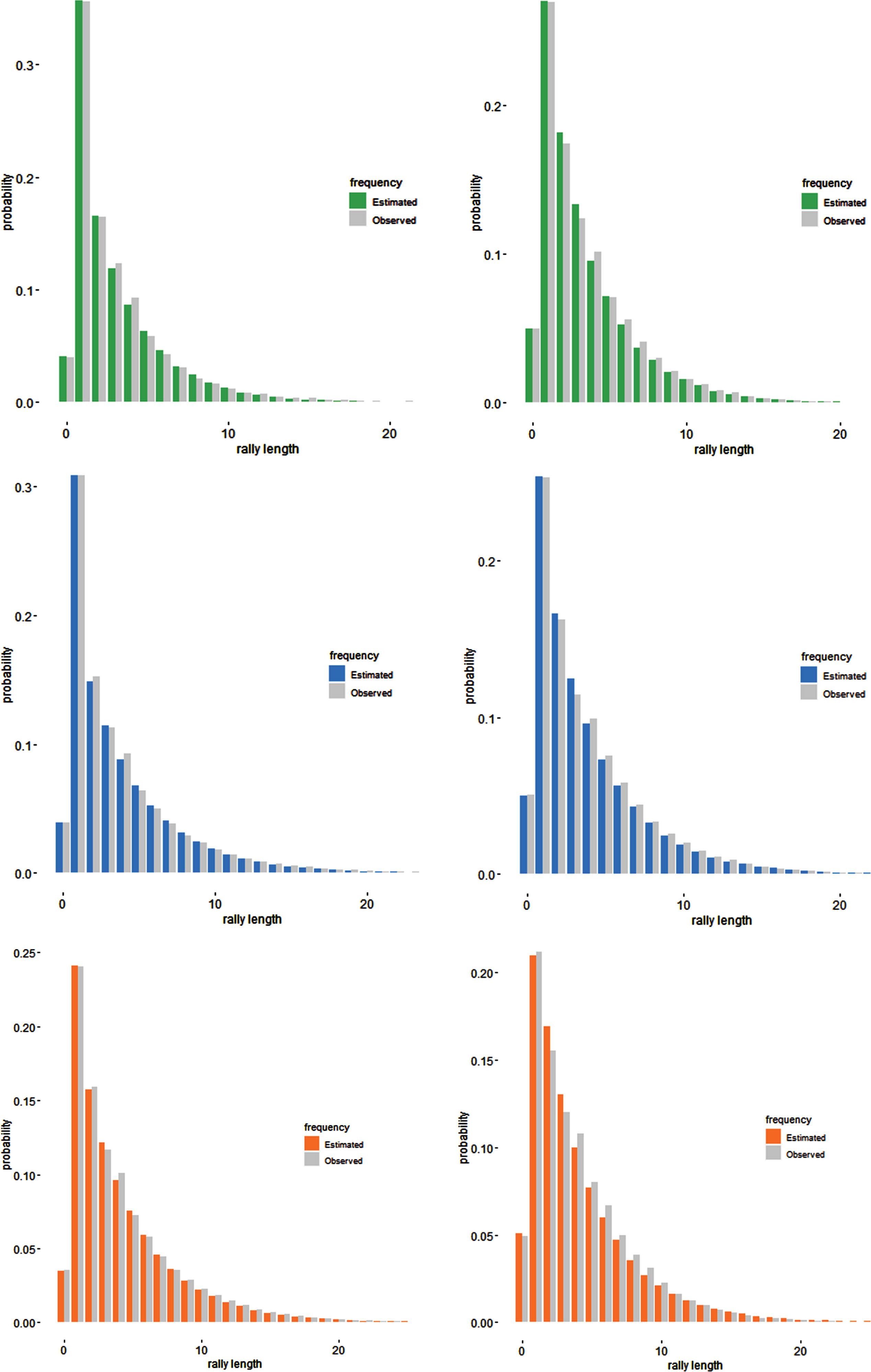
Conditional zomGeom model: observed and estimated distributions of the first 25 rally lengths on grass, hard and clay and for men (left column) and women (right column).

7 Conclusions

In this work we have analyzed the rally length distributions for male and female professional tennis matches. Their characteristics have been studied separately on grass, hard and clay surfaces.

Our study differs from the other (few) available in the literature for the extension of the sample size, giving quite reliable results. In addition, the rally length has not been categorized, but each single value, up to the maximum observed, has been specifically considered. In the Appendix the observed frequencies for each rally length are provided for possible future research.

We have focused on finding the statistical distribution most suitable to describe the observed frequencies. To this end, we have considered both unconditional and conditional models. For the latter, parameters were written as a function of other variables.

Our results point out that the statistical distribution which best fits the data is a conditional zero-one-modified Geometric distribution, whose parameters depend on the probabilities that players win a point at serve and on the players’ heights. The estimated distributions can be considered not significantly different from the observed ones. Results have also shown that the (log) sum of the the players’ heights is the most impacting variable on the rally length distribution.

As a future research it will be interesting to analyze and compare the rally length distributions of individual players. This, in turn, could allow to cluster players according to the features of their the rally length distribution and to define the characteristics of two opponents, possibly for each surface.

In addition, analysing player-specific rally length distributions using the proposed methodology may be useful to define betting strategies. Following the approaches of Candila and Palazzo (2020) or Gao and Kowalczyk (2021), the information contained in the rally length distribution could be included in a wide variety of features that could enter some statistical or machine-learning models. For example, Candila and Palazzo (2020) consider some variables related to the fatigue accumulated by the players in the last matches in order to define a betting strategy. As the tendency to play long rallies is correlated to the match duration and to physical stress, the features of the distribution can provide other variables to include in the model. Likewise, Gao and Kowalczyk (2021) consider composite variables obtained combining simple variables, i.e. the ratio between aces and double faults. Also in this case, one can extract information from the rally length distribution by building suitable indicators. The skewness coefficient or the ratio between the probability that a rally length is shorter than or equal to two and the probability that is is longer than two, are just a couple of possible indicators.

Footnotes

Appendix

Table 15

Women: Absolute observed frequencies for the rally length

Rally	Grass	Hard	Clay
0	3, 279	6, 600	2, 524
1	17, 761	33, 069	10, 806
2	11, 507	21, 219	7, 933
3	8, 186	14, 941	6, 126
4	6, 704	12, 935	5, 516
5	4, 697	9, 914	4, 092
6	3, 699	7, 650	3, 416
7	2, 722	5, 830	2, 544
8	1, 998	4, 412	1, 971
9	1, 426	3, 366	1, 580
10	1, 064	2, 598	1, 156
11	839	1, 949	829
12	541	1, 490	642
13	456	1, 166	508
14	307	850	354
15	193	656	290
16	149	494	200
17	118	367	134
18	63	265	108
19	50	186	94
20	36	147	80
21	32	107	44
22	15	79	33
23	17	48	24
24	13	52	14
25	6	24	18
26	4	25	10
27	3	20	5
28	0	11	5
29	3	7	4
30	2	7	6
31	1	7	0
32	1	5	4
33	0	3	0
34	1	0	1
35	0	2	2
36	0	1	0
37	0	0	1
38	0	0	0
39	0	4	0
40	0	0	0
41	0	0	0
42	0	0	0
43	0	0	0
44	0	1	0
45	0	0	0
46	0	0	0
47	0	0	0
48	0	1	1

Note that in the notation of Carboch et al. (2019) double faults are represented by 1 shot.

In their terminology, the service bonus is the sum of the probabilities that two players have to win the point at serve, while the malus is the absolute difference of the same probabilities.

https://github.com/JeffSackmann/tennis_MatchChartingProject

Digitalized versions of Tables 14 and are available upon request to the authors.

But at at the Australian Open 2013 Gilles Simon and Gael Monfils played a point of 71 strokes. Clearly, this match was not included in our crowdsourced dataset.

The improvement in fitting has been verified ex-post.

References

Bieniek,

, & Kwater,

, 2015, Body height and career win percentage in relation to serve and return games effectiveness in elite tennis players, Scientific Review of Physical Culture, 4(3), 75–80.

Candila,

, & Palazzo,

, 2020, Neural networks and betting strategies for tennis, Risks, 8(6).

Carboch,

, Blau,

, Sklenarik,

, Siman,

, & Placha,

, 2020, Ball change in tennis: How does it affect match characteristics and rally pace in grand slam tournaments? Journal of Human Sport and Exercise, 15, 153–162.

Carboch,

, Siman,

, Sklenarik,

, & Blau,

, 2019, Match characteristics and rally pace of male tennis matches in three grand slam tournaments, Physical Activity Review, 7, 49–56.

Fernandez-Fernandez,

, Sanz-Rivas,

, Fernandez-Garcia,

, & Mendez-Villanueva,

, 2008, Match activity and physiological load during a claycourt tennis tournament in elite female players, Journal of Sports Sciences, 26, 1589–1595.

Fitzpatrick,

, Stone,

J. A.

, Choppin,

, & Kelley,

, 2021, Investigating the most important aspect of elite grass court tennis: Short points, Sports Science & Coaching, 16, 1178–1186.

Gao,

, & Kowalczyk,

, 2021, Random forest model identifies serve strength as a key predictor of tennis match outcome, Journal of Sports Analytics, 7, 255–262.

Gomes,

, Coutts,

, Viveiros,

, & Aoki,

, 2011, Physiological demands of match-play in elite tennis: A case study, European Journal of Sport Science, 11, 105–109.

Heilbron,

D. C.

, 1994, Zero-altered and other regression models for count data with added zeros, Biometrica Journal, 36, 531–547.

10.

Ingram,

, 2021, Rally lengths on the log scale, Martin Ingram’s Blog, https://martiningram.github.io/gp-random-effects-log-scale/.

11.

Kovalchik,

S. A.

, & Ingram,

, 2018, Estimating the duration of professional tennis matches for varying formats, Journal of Quantitative Analysis in Sports, 14(1), 13–23.

12.

Lambert,

, 1992, Zero-inflated poisson regression with an application to defects in manufacturing, Technometrics, 34, 1–14.

13.

Lisi,

, & Grigoletto,

, 2021, Modeling and simulating durations of professional tennis matches by resampling match features, Journal of Sports Analytics, 7(2), 57–75.

14.

Makino,

, Odaka,

, Kuroiwa,

, Suwa,

, & H, S., 2020, Feature selection to win the point of atp tennis players using rally information, International Journal of Computer Science in Sport, 19(1), 37–50.

15.

McCullagh,

, & Nelder,

J. A.

, 1989, Generalized Linear Models. 2nd Edition. Chapman and Hall.

16.

Mlakara,

, & Kovalchik,

, 2020, Analysing time pressure in professional tennis, Journal of Sports Analytics, 6, 147–154.

17.

Mohammadi,

, Sajjadnia,

, Bakouch,

H. S.

, & Sharafi,

, 2021, Zero-and-one inflated poisson-lindley inar(1) process for modelling count time series with extra zeros and ones, Journal of Statistical Computation and Simulation, 92, 2018–2040.

18.

Mullahy,

, 1986, Specification and testing of some modified count data models, Journal of Econometrics, 33(3), 341–365.

19.

Nelder,

J. A.

, & Wedderburn,

R. W.

, 1972, Generalized linear models, Journal of the Royal Statistical Society. Series A., 135(2), 370–384.

20.

Pascual,

J. V.

, 2023, Types of serve stance and height of players.a study of the best servers in history, Coaching & Sport Science Review, 89, 16–20.

21.

Qi,

, Li,

, & Zhu,

, 2019, Modeling time series of count with excess zeros and ones based on inar(1) model with zero-one inflated poisson innovations, Journal of Computational and Applied Mathematics, 346, 572–590.

22.

Vaverka,

, & Cernosek,

, 2013, Association between body height and serve speed in elite tennis players, Sports Biomechanics, 12(1), 30–37.

	Men		Women
Surface	N. of matches	N. of points	N. of matches	N. of points
Grass	710	70,333	912	65,705
Hard	3,332	290,340	1,833	130,235
Clay	1,709	142,253	686	51,449
Total	5,751	503,946	3,431	247,389

On the distribution of rally length in professional tennis matches

Abstract

Keywords

1 Introduction

2 Literature review

3 The dataset

Table 1 Matches and points sample sizes for men and women and for different surfaces Men Women Surface N. of matches N. of points N. of matches N. of points Grass 710 70,333 912 65,705 Hard 3,332 290,340 1,833 130,235 Clay 1,709 142,253 686 51,449 Total 5,751 503,946 3,431 247,389

4.1 Unconditional models

Footnotes

Appendix

References

Table 1
Matches and points sample sizes for men and women and for different surfaces

Men Women

Surface N. of matches N. of points N. of matches N. of points

Grass 710 70,333 912 65,705

Hard 3,332 290,340 1,833 130,235

Clay 1,709 142,253 686 51,449

Total 5,751 503,946 3,431 247,389