Sage Journals: Discover world-class research

Abstract

We analyse data from the Euroleague, between the 2000–1 season and the 2021–2022 season. Our aim is to identify the game-related statistics which discriminate between successful teams from unsuccessful ones, at a season-level, where success is identified as either (i) qualification to playoffs, or (ii) participation in the Final Four. We use both statistical and machine learning methods for the analysis. A logistic regression model identified, in decreasing order of significance, points per possession, defensive rebounds, possessions per game, fouls drawn, successful free throw percentage, offensive rebounds percentage and steals, as the most important factors regarding qualification to playoffs. For the Final Four, the key determinants were effective field goal percentage, total rebounds, pace, fouls drawn, turnovers, steals and blocks. In particular, we have found that the number of possessions per game and pace are negatively correlated with a team's season success. Among the machine learning methods, Support Vector Machines gave the best results for classifying the teams. We also discuss how the top performances of individual players affect season-long success of their teams. Some very high individual performances came from players whose team did not proceed further in the competition. For a team to qualify for the subsequent phases, it is not enough to have one player with a high scoring average or performance index rating.

Keywords

Euroleague game-related statistics logistic regression machine learning

Introduction

Over the last decades, the use of statistics in sports has grown enormously: this is partly due to the rapid increase in the speed and computational power of statistical algorithms, but also reflects the necessity to analyse and learn from the vast amounts of data that become available on a daily basis. In an article in Statistical Science Aiding Sports of the American Statistical Association we read that “the use of statistical science in sports continues to evolve, with its power and utility well established in certain areas but providing new challenges as a result of fresh sources and ever-increasing amounts of data” (ASA, 2017). It is thus widely acknowledged that statistical methods and results assist in evidence-based decision making and offer the opportunity, both for coaches and athletes, to monitor and improve their performance. In addition, newly established tools and techniques from machine learning and data science are particularly suited for large amounts of data, a typical phenomenon in today's sports world.

Traditionally, basketball has been one of the most analysed sports using statistics. As a result, performance analysis in basketball is currently an essential tool for coaches and technical staff (García et al., 2013). In a number of recent studies, interest has focused on the key performance indicators that discriminate between winning and losing teams, in various national and international competitions (Akers et al., 1991; Csataljay et al., 2009; de Rose, 2004; Gómez et al., 2008; Karipidis et al., 2001; Lorenzo et al., 2010). Although in most studies it was found that field goal percentage and defensive rebounds are the key factors determining success (Akers et al., 1991; Gómez et al., 2008; Tsamourtzis et al., 2002), recent research suggests that the most influential game-related statistics may vary according to home and away games, regular season and playoff, final score differences, team gender, level of competition (e.g., Euroleague, National Basketball Association) and age of the players (Lorenzo et al., 2010). In the present study we have analysed data from the top European competition in basketball, the Euroleague, throughout the period 2000–2022. We have thus focused on season-long success rather than win at individual games, where ‘success’ in our context has been identified as either (i) qualification to the playoff phase; or (ii) participation in the Final Four of the competition.

In a recent study, Mandić et al. (2019) performed a multi-season (2000–2017) comparison between the NBA and the Euroleague. The main differences they found had to do with the pace of the game; offenses in the NBA are shorter but less worked out. The latter is exemplified by the higher 2-point percentage in the Euroleague (+3.7%, as recorded by the authors). Another recent study, using meta-analysis and focusing on discriminant analysis methods is Canuto and de Almeida (2022). Some articles studying performance indicators for the Euroleague are Dogan and Ersoz (2019), Marmarinos et al. (2016), Mikolajec et al. (2021) and Štrumbelj et al. (2013). In particular, Marmarinos et al. (2016), aiming to investigate which factors were statistically significant for the qualification of a team to the Euroleague playoffs, collected data from 1514 games of the 2012–15 seasons, and by using discriminant analysis concluded that defensive rebounds, offensive and defensive efficiency, assists and turnovers were the key discriminant factors. Dogan and Ersoz (2019), using also linear discriminant analysis, investigated which factors play a decisive role in the qualification of teams through the Euroleague rounds. They collected data for the 2010–2017 seasons and concluded that the percentage of successful two-point shots, defensive rebounds, fouls in favor and blocks in favor are the elements with the greatest contribution for the Top 16 round. Regarding the playoffs, the biggest contributors were successful two-point shots, blocks made and turnovers. For Final Four qualification, successful three-point shots had the largest impact. Mikołajec et al. (2021) searched for the factors associated with the performance of 10 Euroleague teams over 13 seasons. Using regression analysis, they concluded that the number of two-point shots made and attempted, the number of free throws made, the number of three-point shots made and attempted, the assists and the fouls had the greatest impact. Ibañez et al. (2008) found that for the Spanish League, assists, steals and blocks are the most important factors separating successful from unsuccessful teams.

The main aims of the present article are:

To investigate how boxscore statistics in Euroleague vary through time between 2000–01 and the 2021–22 season;

To identify, among these statistics, the key factors that affect a team's success (qualification to playoffs – Final Four) in a season;

To examine whether the performance of the top players in a season affects the success of their teams.

More specifically, we examine season-long success for all teams that participated in the Euroleague between the 2000–1 season and the 2021–22 season, in relation to game-related statistics, mostly but not exclusively those available in a boxscore. In particular, the data we have used as potential determinants for success in a season are annual averages, per team, in field shooting, defensive and offensive rebounds, assists, steals, blocks etc. (see the list in Table 1). Of course, with today's technology and the availability of big data facilities and algorithms one might be tempted to use individual game statistics rather than annual averages. For measuring season-long success, we advocate the use of the latter for two reasons: (i) when dealing with large amounts of data, annual averages give a clear and concise view of the key features of the data which is easy to understand intuitively and facilitates comparisons between different teams, years etc; (ii) values for individual games are hardly ever normally distributed. Yet several statistical methods (linear regression, analysis of variance and covariance, linear discriminant analysis) rely on the assumption of normality. The use of annual averages instead of individual boxscore values removes that barrier in view of the Central Limit Theorem (CLT) of probability theory. In addition to these, in the present context we note that the number of games played by a team is not the same through the years while, for a particular year, it also varies among different teams.

Table 1.

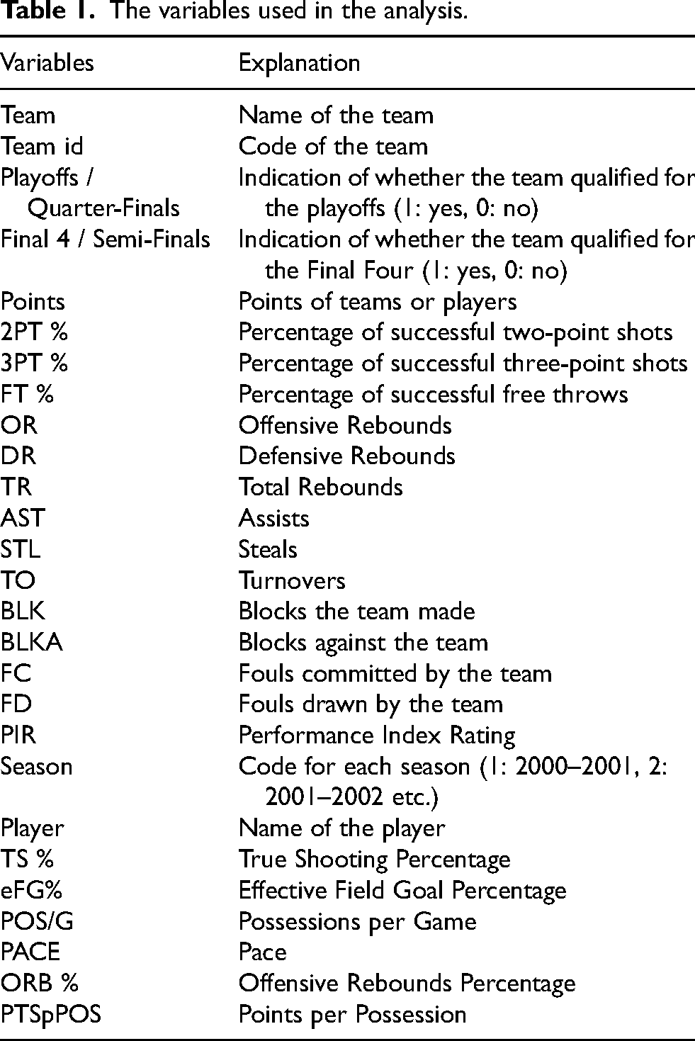
The variables used in the analysis.

Variables	Explanation
Team	Name of the team
Team id	Code of the team
Playoffs / Quarter-Finals	Indication of whether the team qualified for the playoffs (1: yes, 0: no)
Final 4 / Semi-Finals	Indication of whether the team qualified for the Final Four (1: yes, 0: no)
Points	Points of teams or players
2PT %	Percentage of successful two-point shots
3PT %	Percentage of successful three-point shots
FT %	Percentage of successful free throws
OR	Offensive Rebounds
DR	Defensive Rebounds
TR	Total Rebounds
AST	Assists
STL	Steals
TO	Turnovers
BLK	Blocks the team made
BLKA	Blocks against the team
FC	Fouls committed by the team
FD	Fouls drawn by the team
PIR	Performance Index Rating
Season	Code for each season (1: 2000–2001, 2: 2001–2002 etc.)
Player	Name of the player
TS %	True Shooting Percentage
eFG%	Effective Field Goal Percentage
POS/G	Possessions per Game
PACE	Pace
ORB %	Offensive Rebounds Percentage
PTSpPOS	Points per Possession

Another question that we address in the following sections is the extent to which the individual performance of the top players may lead their team to overall success for a season. For an individual game which is closely contested, it is usually the top players for each team who, in the deciding final minutes, or even seconds of a game, step up in order to lead their team to victory. We attempt to look back at what has happened so far in the Euroleague: do the top performers for each season belong to teams that qualified for the playoffs/Final Four or not?

Methods

The data of this article refer to averages of players and teams competing in the Euroleague, starting from the 2000–2001 season (when the competition as it is known today was established) up to the 2021–2022 season. During this period, a total of 87 teams from 19 countries have participated, at least for one season. Some teams have used several different names in that period due to sponsorship deals. In the analysis, the teams are presented under their current names.

From 2000 to 2022, the Euroleague has underwent several format changes, reflecting the evolution of European basketball. In the early 2000s, the competition featured a regular season with multiple groups, followed by a Top 16 stage and a subsequent knockout phase leading to the Final Four. In 2004–2005, an extra round was introduced, culminating in a playoff phase and the Final Four. The 2008–2009 season saw the adoption of a new format, with a round-robin regular season followed by playoffs and the Final Four. This structure remained for several years, with slight modifications to the number of teams and games. In the 2016–2017 season, a radical change occurred as the Euroleague transitioned to a league format with a round-robin system among 16 teams (today 18 teams), followed by playoffs and the Final Four.

As mentioned already, in the following sections we focus on the key factors affecting qualification to the playoffs and the Final Four. We note that from the 2001–2002 season to the 2003–2004 season, there was no playoffs phase, while the 2019–2020 season was permanently discontinued due to covid-19. For this reason, we used the data for the 2001–2004 and 2019–2020 seasons only in the descriptive analysis and excluded these seasons from the remaining parts of the data analysis.

In Table 1 we list the variables used in our analysis.

The Performance Index Rating (PIR) is calculated as follows: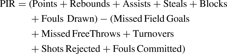

\begin{aligned} PIR = & (Points + Rebounds + Assists + Steals + Blocks \\ + Fouls Drawn) - (Missed Field Goals \\ + Missed Free Throws + Turnovers \\ + Shots Rejected + Fouls Committed) \end{aligned}

The TS % is calculated as (Points × 50) / [(FGA + 0,44 * FTA)], where FGA are the field goals attempted and FTA the free throws attempted. The eFG% is given by (FG + 0.5 * 3PT) / FGA and the ORB% is equal to 100 * [Player ORB * (Team Minutes / 5)] / [Player Minutes * (Team ORB + Opponent DRB)]. We have pulled our data from the official site of EuroLeague (https://www.euroleaguebasketball.net/euroleague/) and the site RealGM (https://basketball.realgm.com/).

The main methods employed in the analysis are:

Descriptive statistics and hypothesis testing. First, we look at the temporal variation of boxscore data (averages). Further, we perform two-sample t-tests to see which characteristics differ between the teams, or players, who qualified (for playoffs or the Final Four) and those who did not.

Correlations. By looking at pairwise correlations between the variables used in the analysis, we examine the degree of relationship that exists between them (if any). In particular, we investigate which variables are more closely related with the Performance Index Rating (PIR) which is, to a large extent, indicative of a team's success.

Logistic regression analysis. In such a model, the response variable is binary. We have tried to fit two logistic regression models to our annual average data for the teams, one using qualification in the playoffs and one for participation in the Final Four. Although discriminant analysis has been favored by many authors to analyze basketball data, we prefer to use logistic regression which is generally more robust, both to assumptions and outliers.

Machine learning methods. We use classification and clustering methods (feature selection, cluster analysis, random forest, support vector machines) to identify the variables which distinguish between successful and unsuccessful teams.

The statistical package R (version 4.1.1) was used throughout for the analysis. Unless otherwise stated, a 5% significance level has been used for the statistical tests.

Results

Team performance indicators

In this subsection we analyze team statistics while subsequently we look at the effect of individual players.

Temporal evolution of the indicators

Table 2 shows the minimum value, first quartile, median, mean, third quartile and maximum value, for the mean of the variables (team statistics) for the entire period under consideration.

Table 2.

Descriptive statistics for the annual averages of the variables.

	Min.	1st. Qu.	Median	Mean	3rd. Qu.	Max.
Points	73.57	74.86	76.98	77.16	79.19	80.72
2PT %	50.10	50.83	51.62	51.77	52.66	53.70
3PT %	33.23	35.20	35.38	35.62	36.29	37.91
FT %	70.95	72.59	73.65	74.20	75.30	79.67
Offensive Rebounds	9.33	9.80	10.00	9.99	10.26	10.54
Defensive Rebounds	21.48	22.25	22.84	22.80	23.27	24.17
Total Rebounds	31.14	32.02	32.89	32.80	33.58	34.72
Assists	10.71	12.70	13.62	14.50	17.05	17.64
Steals	5.72	6.39	6.77	7.72	8.88	10.98
Turnovers	11.81	12.84	13.30	13.33	13.96	14.77
Blocks	2.23	2.42	2.52	2.51	2.61	2.72
Blocks Against	2.01	2.44	2.57	2.54	2.74	2.83
Fouls Committed	19.47	20.71	21.36	21.56	22.14	24.14
Fouls Drawn	19.22	20.41	20.91	21.11	21.80	22.85
PIR	75.35	77.91	80.16	81.04	83.94	89.04
Possessions per Game	68.67	70.05	70.55	70.73	71.13	73.92
Pace	68.14	69.59	70.08	70.30	70.43	73.95
Points per Possession	1.04	1.07	1.08	1.09	1.12	1.16

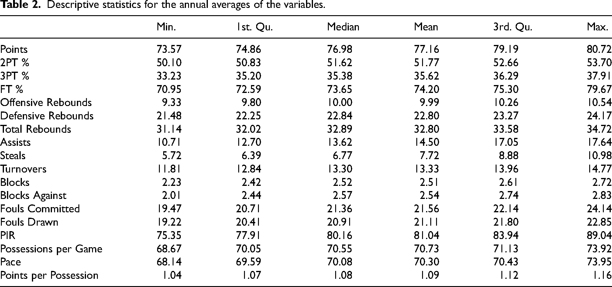
In order to have an insight as to how these variables vary through time, we present some time series plots (Figure 1). Some conclusions we can draw are the following: The most prominent increase through time seems to be for FT% and assists. Further, from the 2010–2011 season onwards there is a sudden, upward trend for points, points per possession, two-point and three-point shooting percentages, defensive rebounds, total rebounds and the overall PIR for the teams. This may be due to the fact that since the 2010–2011 season, there have been some changes in the rules of the game.

Figure 1.

Time series plots of the variables over the seasons.

On the other hand, we observe in Figure 1 that there is a downward trend with time regarding steals, turnovers, fouls committed, fouls received, pace and possessions per game. In particular, the number of fouls (committed and received) has an almost linear relation with time, with a negative slope, a fact which is reinforced by the correlation coefficient of these variables with the variable for seasons (−0.89 and −0.86 respectively).

The blocks that teams made and received seem to peak around the 2014–2015 season and then follow a downward trend. Offensive rebounds exhibit a lot of fluctuation with time. Ibañez et al. (2018) came to similar conclusions regarding the relationship between changes in regulations and an increase in shooting accuracy rates in general, as well as a reduction in turnovers, steals and fouls committed by players, among others.

Next, we used a graphical representation known as Chernoff faces (Chernoff, 1973), to visualize similarities and differences among the seasons.

Seasons 17 to 20 are quite similar to each other, e.g., in terms of offensive and defensive rebounds, assists, blocks and points per possession. Seasons 11, 12 and 15 are also similar, in turnovers and pace among others. Season 21 stands out with a high PIR, marked by a distinct smile, indicating it was a season with very high performances overall. Seasons 1 and 2 show a more conservative approach in their pace and points per possession, as reflected in their simpler hair styles. The most dissimilar seasons are 11 and 21. Overall, seasons which were chronologically closer seem to have the most similarities in terms of their characteristics.

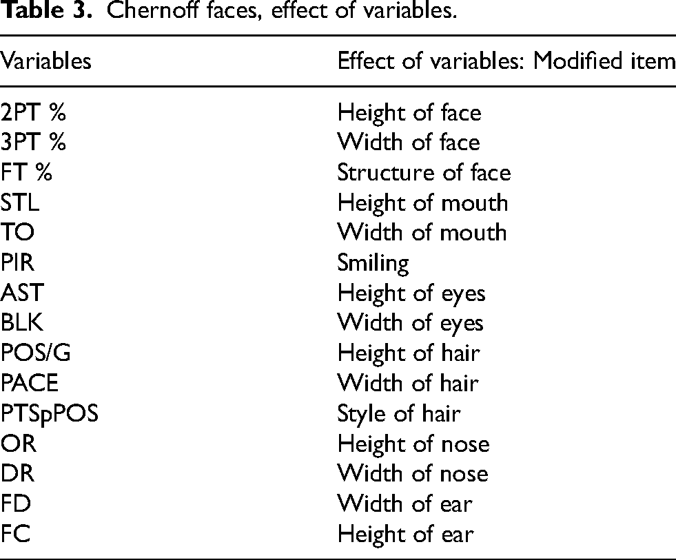
Table 3 is the key to understanding the face characteristics in Figure 2.

Figure 2.

Chernoff faces for each season.

Table 3.

Chernoff faces, effect of variables.

Variables	Effect of variables: Modified item
2PT %	Height of face
3PT %	Width of face
FT %	Structure of face
STL	Height of mouth
TO	Width of mouth
PIR	Smiling
AST	Height of eyes
BLK	Width of eyes
POS/G	Height of hair
PACE	Width of hair
PTSpPOS	Style of hair
OR	Height of nose
DR	Width of nose
FD	Width of ear
FC	Height of ear

Comparison of qualified and non-qualified teams in playoffs phase

We have performed two-sample t-tests to examine differences in performance indicators between qualified and non-qualified teams for the playoffs. The results are given in Table 4. For 18 variables there is a significant difference at the 5% level, while in 15 among these the difference is significant at the 0.1% level; the relatively large sample sizes enable to identify even small differences between the two groups. In most cases qualified teams perform much better than non-qualified ones. However, it is interesting to note that for two indicators (pace and possessions per game), the non-qualified teams have a higher average and the difference is significant. This seems to be in accordance with the situation at the other side of the Atlantic. For instance, in the last season of the NBA (2023–24) the two teams with the highest numbers of possessions per game were the Washington Wizards and the San Antonio Spurs which had among the worst regular season performances in that season (winning-losing records were 15–67 and 22–60 respectively). On the other hand, among the 5 teams with the best record in the regular season, only one (Oklahoma City Thunder) was in the top 10 in terms of POS/G.

Table 4.

Significantly different to qualified teams * p < 0.05, ** p < 0.01, *** p < 0.001.

Variables	Non-qualified teams (n = 252)	Qualified teams (n = 144)
Points	74.84 ± 4.57***	79.19 ± 4.31
2PT %	50.57 ± 2.75***	53.25 ± 2.54
3PT %	34.47 ± 2.82***	36.91 ± 2.64
FT %	73.72 ± 4.46*	74.74 ± 4.17
DR	22.48 ± 1.81***	23.70 ± 1.44
TR	32.60 ± 2.41***	33.52 ± 1.98
AST	13.93 ± 2.71***	15.40 ± 2.67
STL	7.65 ± 2.37	7.72 ± 2.28
TO	13.81 ± 1.61***	12.76 ± 1.35
BLK	2.38± 0.74***	2.80 ± 0.67
BLKA	2.71± 0.60***	2.47 ± 0.48
FC	21.52± 2.01*	21.11 ± 1.96
FD	20.58 ± 1.71***	21.57 ± 1.69
PIR	76.03 ± 9.38***	87.48 ± 8.11
PIR_INDIV	16.01 ± 3.48*	16.65 ± 2.69
PIR_BEST_FIVE	11.56 ± 1.55***	12.46 ± 1.32
TS %	54.98 ± 2.68***	58.03 ± 2.50
eFG %	51.00 ± 2.64***	54.00 ± 2.58
PACE	70.45 ± 2.12**	69.86 ± 2.16
ORB %	28.88 ± 3.68	29.33 ± 3.14
POS/G	71.00 ± 2.83**	70.25 ± 2.13
PTSpPOS	1.05 ± 0.06***	1.13 ± 0.05

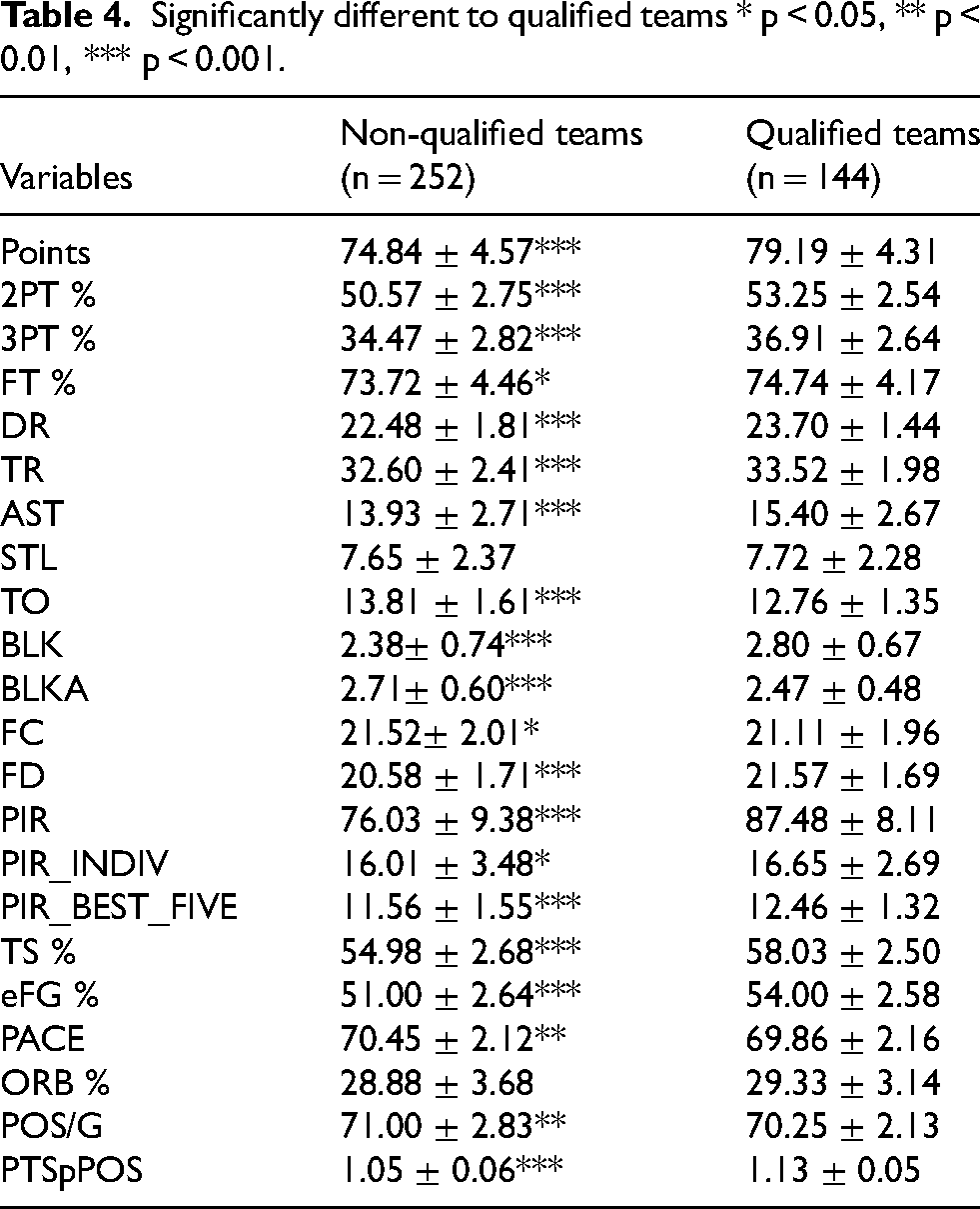
The picture is similar when considering the pace (in the 2023–24 season, Wizards and Spurs were ranked 1^st and 3^rd, while the champions Celtics were 20^th among NBA teams). It therefore seems that for both the world's top basketball competitions, teams with high scores in these two indicators are less likely to have a good overall performance in a season.

Normality and correlations

As the data we used in the analysis are the yearly averages for each team, we expect that the normal distribution offers a suitable choice for these values. Since the parameters of the normal distribution are not known, we used a variant of the Kolmogorov-Smirnov test, known as the Lilliefors test, to test for normality (Conover, 1999). The only variables that the assumption of normality is rejected are three-point shots (p = 0.018) and steals (p = 0.001).

Moreover, we expect the PIR to be the variable that summarizes a team's performance in a game, as it is based on all other boxscore statistics. Figure 3 presents scatterplots between the PIR and each of the other variables. We notice that there is strong, positive correlation between PIR and points, points per possession, the percentage of free throws, 2- and 3-point %, and assists. A strong, negative correlation with turnovers can also be seen. In addition, a low positive correlation appears to exist between PIR and offensive rebounds, defensive rebounds, and total rebounds. Variables exhibiting a low, negative correlation with PIR are steals, blocks in favor of the teams, blocks against the teams, fouls committed, fouls won, possessions per game and pace.

Figure 3.

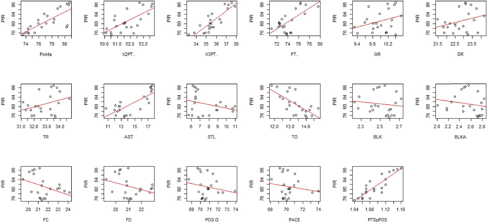
Scatter plots of the variables with the PIR.

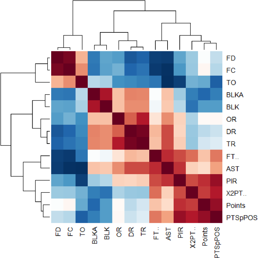
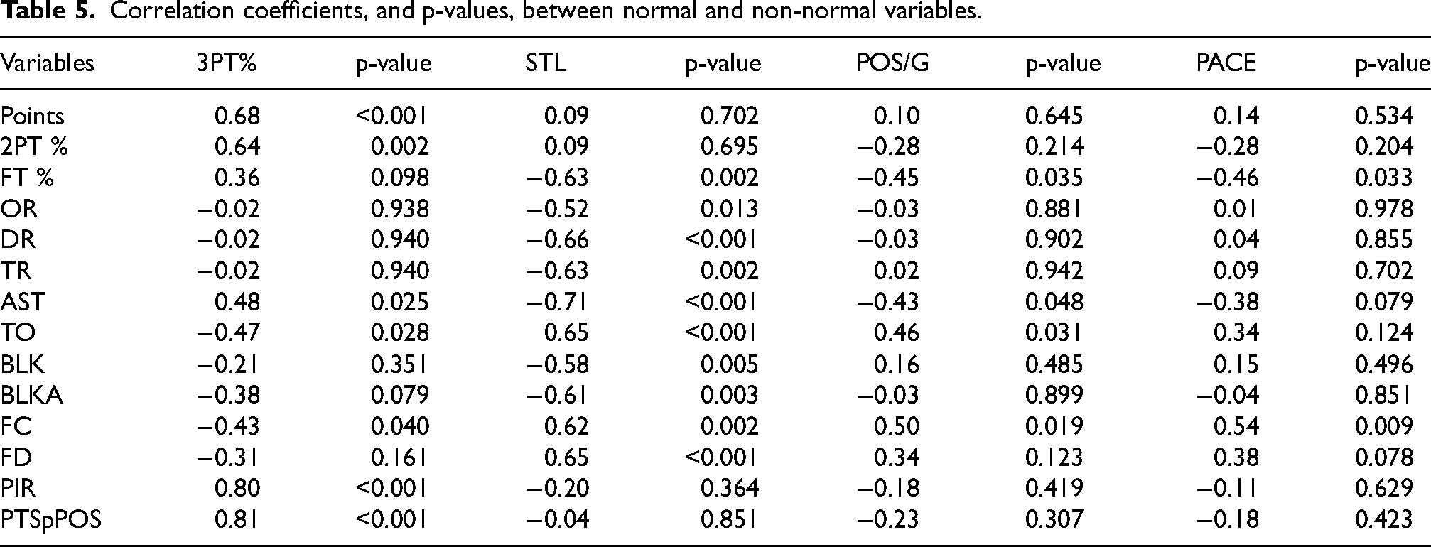
Next, we look at the pairwise correlations between all variables. For the variables that were found to comply with the assumption of the normal distribution, Figures 4 and 5 depict a correlogram as well as a heatmap, using Pearson's correlation coefficient. For the remaining variables, 3PT%, steals, possessions per game and pace, Table 5 gives their correlation with each of the other variables, along with the p-value. The Spearman correlation coefficient was used in this case, and the null hypothesis is that there is no correlation between the variables. As we see from Table 4, the coefficients between 3PT% and each of Points, 2PT%, AST, TO, FC, PIR and PTSpPOS are significant. Coefficients between STL and FT%, OR, DR, TR, AST, TO, BLK, BLKA, FC and FD are also significant. Other significant correlations are between POS/G and FT%, AST, TO and FC, as well as the correlations between PACE and FT%, FC. It is of course expected to observe a high, positive relationship between the percentage of three-points shots and points; it is however worth noting that the correlation between 3PT% and 2PT% is also highly significant, demonstrating that teams which shoot well from outside have also high percentages inside the three-point arc. We also note the strong negative correlation between steals and assists, i.e., teams that make a lot of steals seem not to give out many assists, since they would probably manifest “fastbreak” offensive scenarios.

Figure 4.

Correlogram for the normal, quantitative variables.

Figure 5.

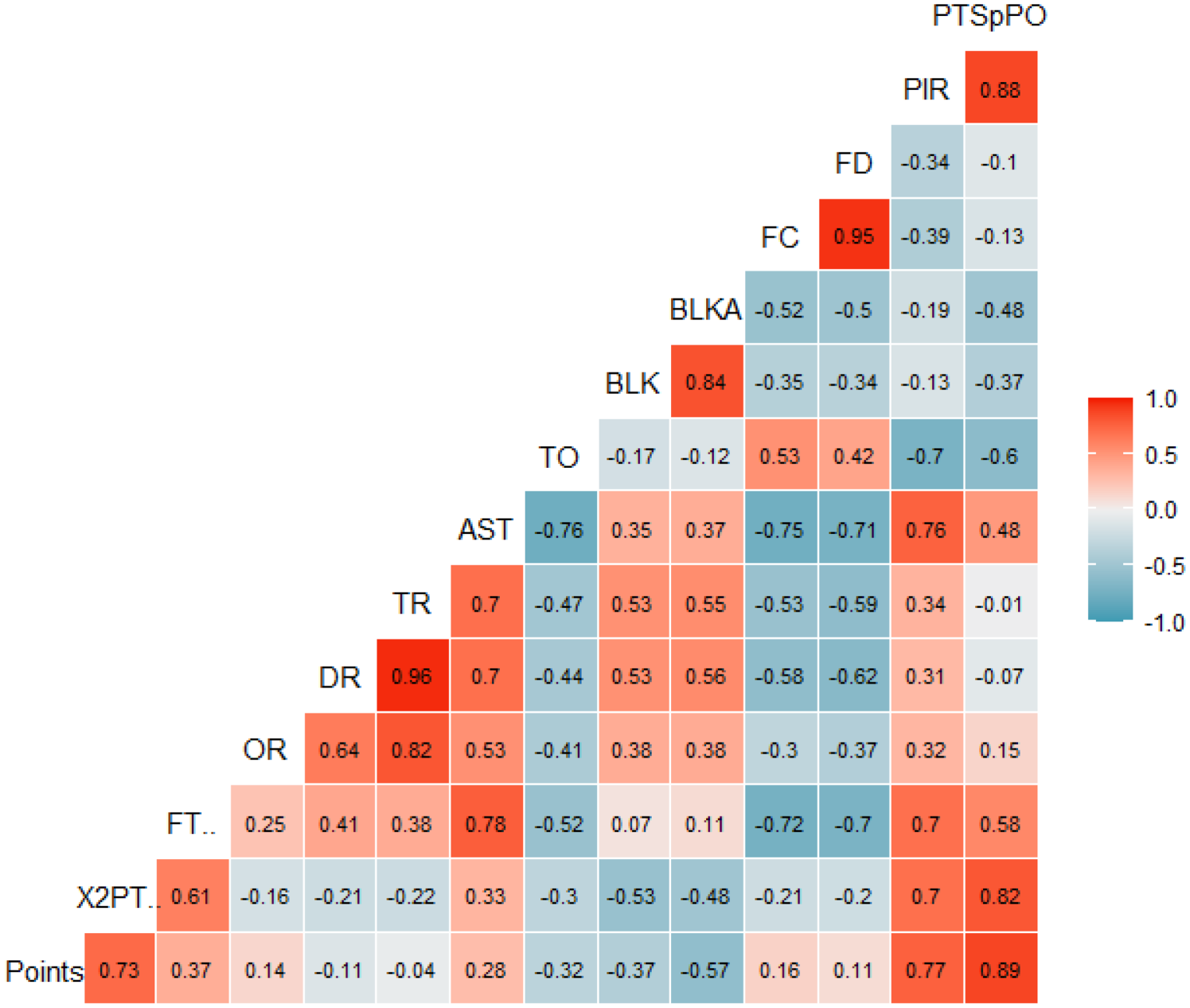
Heatmap for the normal, quantitative variables.

Table 5.

Correlation coefficients, and p-values, between normal and non-normal variables.

Variables	3PT%	p-value	STL	p-value	POS/G	p-value	PACE	p-value
Points	0.68	<0.001	0.09	0.702	0.10	0.645	0.14	0.534
2PT %	0.64	0.002	0.09	0.695	−0.28	0.214	−0.28	0.204
FT %	0.36	0.098	−0.63	0.002	−0.45	0.035	−0.46	0.033
OR	−0.02	0.938	−0.52	0.013	−0.03	0.881	0.01	0.978
DR	−0.02	0.940	−0.66	<0.001	−0.03	0.902	0.04	0.855
TR	−0.02	0.940	−0.63	0.002	0.02	0.942	0.09	0.702
AST	0.48	0.025	−0.71	<0.001	−0.43	0.048	−0.38	0.079
TO	−0.47	0.028	0.65	<0.001	0.46	0.031	0.34	0.124
BLK	−0.21	0.351	−0.58	0.005	0.16	0.485	0.15	0.496
BLKA	−0.38	0.079	−0.61	0.003	−0.03	0.899	−0.04	0.851
FC	−0.43	0.040	0.62	0.002	0.50	0.019	0.54	0.009
FD	−0.31	0.161	0.65	<0.001	0.34	0.123	0.38	0.078
PIR	0.80	<0.001	−0.20	0.364	−0.18	0.419	−0.11	0.629
PTSpPOS	0.81	<0.001	−0.04	0.851	−0.23	0.307	−0.18	0.423

Logistic regression

We have used logistic regression in order to identify the key determinants for a team's success in a season. In logistic regression the response variable is binary, taking values 1 (‘success’) and 0 (‘failure’). We used annual data for each team and identified “success” in two ways: (a) qualification in the playoffs; (b) participation in the Final Four. As potential explanatory variables we have used the variables listed in Table 1. The results are presented separately for each of these two cases.

Qualification to playoffs

As a first step, we used a stepwise procedure so that significant variables, for playoff qualification, enter the model successively. Trying to fit a model using all variables in Table 1, this procedure identified PIR as the most significant variable (p-value $≅ 10^{- 11})$ , followed by AST, STL, FT, FC, Points, TO, 2PT%. Of course, we expect PIR to be very closely related to a team's qualification, however the resulting model is largely problematic. PIR is just a linear combination of the other variables, so the model exhibits multicollinearity (Senaviratna and Cooray, 2019). Using the function vif from package ‘car’ in R, the value of the variance inflation factor (VIF) is 10.32, so the model is unacceptable. We have therefore excluded PIR and points from the analysis. In addition to all the remaining variables in Table 1, we have included two more variables as potential explanatory variables for qualification: (i) the PIR of the top player, that is the player with the highest Performance Index Rating for the specific team and year under consideration; (ii) the average rating of a team's top five players in a specific year. However, neither of these variables was found to be significant.

The stepwise procedure selected seven variables for inclusion in the model. In order of their significance, these are: PTSpPOS, DR, POS/G, FD, FT%, ORB% and STL. The coefficient of POS/G is negative (−0.4347, with a standard error 0.08863), indicating that an increase in the number of possessions per game decreases the estimated probability for qualification. Testing the overall fit of the model with the Hosmer – Lemeshow test, the model was found adequate (p-value = 0.158). The value of McFadden's R² (Cox and Snell, 1989) for the model is 0.384. The ROC curve, which is shown on the left graph of Figure 6 underlines that the model fits the data well (area under curve = 0.885).

Figure 6.

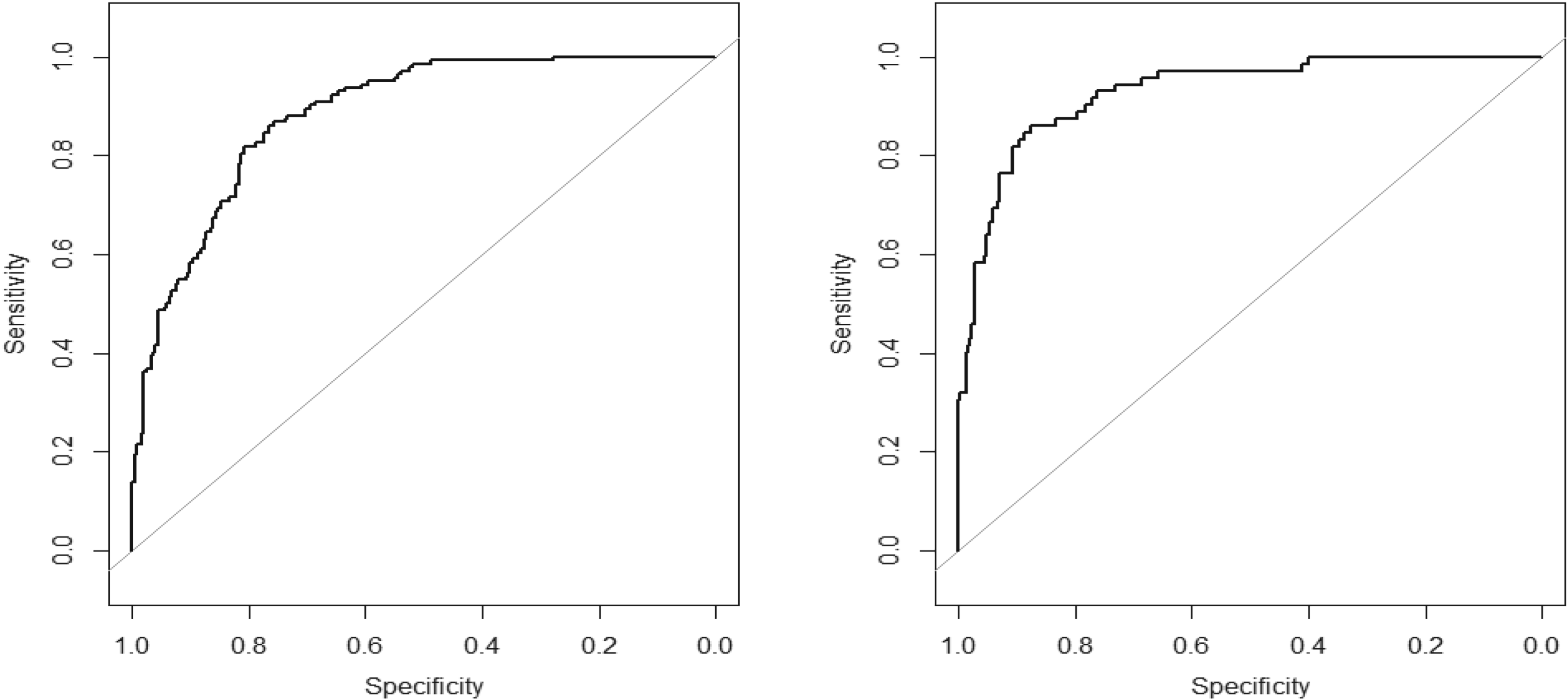
ROC curves based on logistic regression for qualification to playoffs (left) and the final four (right).

Qualification to the final four

A similar logistic regression analysis was carried out in order to determine the factors that affect qualification to the Final Four. Again, PIR and Points were excluded from the model to ensure that multicollinearity is absent. Apart from the other variables in Table 1, we have considered the best player and the top 5 players in each team as explanatory variables for qualification; again, neither of these was significant. The stepwise procedure selected a model with seven explanatory variables. In order of their selection, these were eFG%, TR, PACE, FD, TO, STL and BLK. The adequacy of the model was examined through the Hosmer—Lemeshow test (p-value = 0.1812). The value of McFadden's R square for this model is 0.480. The ROC curve, shown on the right graph of Figure 6, demonstrates further the performance of the model (area under curve = 0.93).

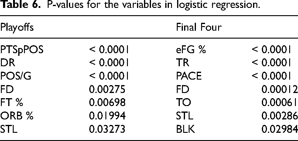
Finally, Table 6 gives, for each of the two logistic regression models, the selected variables and their corresponding p-values. It is perhaps interesting to observe that FD and STL were selected in both cases. The first three variables for Playoffs phase and three for Final Four have a p-value less than or equal to 10⁻⁴. Thus, according to the logistic regression models, there is very strong evidence that these variables are related to a team's success.

Table 6.

P-values for the variables in logistic regression.

Playoffs		Final Four
PTSpPOS	< 0.0001	eFG %	< 0.0001
DR	< 0.0001	TR	< 0.0001
POS/G	< 0.0001	PACE	< 0.0001
FD	0.00275	FD	0.00012
FT %	0.00698	TO	0.00061
ORB %	0.01994	STL	0.00286
STL	0.03273	BLK	0.02984

Machine learning

We also employ machine learning methods to extract further information from the data. In particular, after choosing the appropriate variables (feature selection) which are useful for our algorithms, we use clustering techniques to identify patterns and groups of observations with similar characteristics in the data; in addition, we use classification techniques, in order to fit appropriate classification models for qualification in the two phases of the competition that we consider.

Feature selection with the Boruta algorithm

Among the various machine learning algorithms for feature selection, we have used the Boruta algorithm. The purpose of feature selection is to reduce the number of variables (features) in a dataset by identifying features that principally influence the outcome variable. This algorithm was introduced in Kursa and Rudnicki (2010), and it is based on the Random Forest Classifier algorithm.

Considering qualification to the playoff phase first, our variables were classified into three levels, which are indicated on the left part of Figure 7 by their respective colors. The variables in green are those which have been confirmed by the random forest algorithm. Therefore, the most important variables are points per possession, PIR, effective field goal percentage, true shooting percentage, the percentage of successful 2-PT shots, defensive rebounds, fouls won by the teams, points, blocks, the percentage of successful 3-PT shots, turnovers, possessions per game, pace and the average PIR of the top five players for each team. Assists and total rebounds are tentative variables, i.e., variables that are at the discretion of the analyst to include them in the study, and whose contribution to the model is under investigation. The remaining variables are not approved by the classifier. Finally, there are three shadow features, which are not real variables, they are just useful in the process of deciding whether a variable is significant or not.

Figure 7.

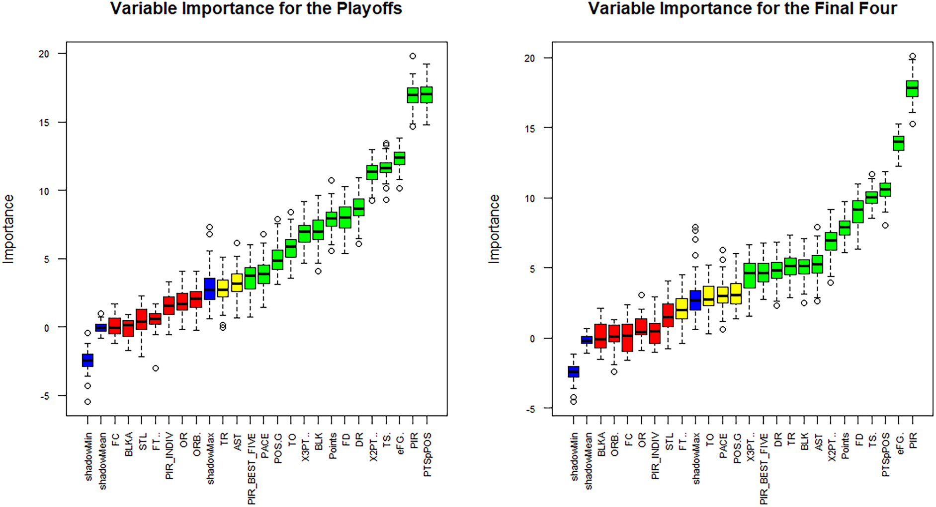
The importance of the variables using the boruta method.

Working similarly, we concluded that the most important variables for the Final Four phase are PIR, effective field goal percentage, points per possession, true shooting percentage, fouls drawn, points, 2-PT%, assists, blocks, total rebounds, defensive rebounds, the average PIR of the top five players for each team and 3-PT%, as shown on the right part of Figure 7.

We note that the Boruta method for feature selection does not explicitly consider the correlation between variables when determining their importance. The main purpose of the algorithm is to identify all significant variables for predicting a response, and significance here entails that correlation is higher than that of the attributes which are randomly generated by the algorithm. Thus, rather than finding a minimal optimal set of attributes, the method tackles the so-called all relevant problem by finding all strongly and weakly relevant variables (Kursa and Rudnicki, 2011).

Clustering

The first step we took before starting our analysis with clustering techniques was to normalize our data. We have used two clustering methods: the k-means method and hierarchical agglomerative clustering. Since the first method gave slightly better results, we report only these below.

The method of k-means clustering is very popular in data mining and machine learning. The basic idea is to divide a set of n data points into k clusters, where k is a user-defined parameter. Various techniques can be used to select the appropriate value for k, such as the elbow method and silhouette analysis. With the elbow method, we plot the within-cluster sum of squares (WCSS) as a function of the number of clusters k and find an “elbow” in the graph. The silhouette method evaluates the quality of the clustering by calculating a “silhouette coefficient” for each data point. This coefficient measures how similar a data point is to points in its own cluster compared to points in other clusters (Tan et al., 2018). In our case, both methods suggested clearly two as the optimal number of clusters.

Applying the k-means algorithm, we obtained the following about the distribution of our data in the two clusters. Among the 252 teams that did not qualify for the playoffs, 162 teams were in cluster 1 and 90 teams were in cluster 2. Out of 144 teams that qualified for the playoffs, 24 teams were in cluster 1 and 120 teams were in cluster 2.

Our data set contains more than two variables, so we cannot use a classical scatter plot to depict them. One solution is to reduce the number of dimensions by applying a dimensionality reduction algorithm, such as principal component analysis (PCA), which creates new variables that are linear combinations of our original variables and try to carry as much information (variability) as possible from the original dataset (Figure 8).

Figure 8.

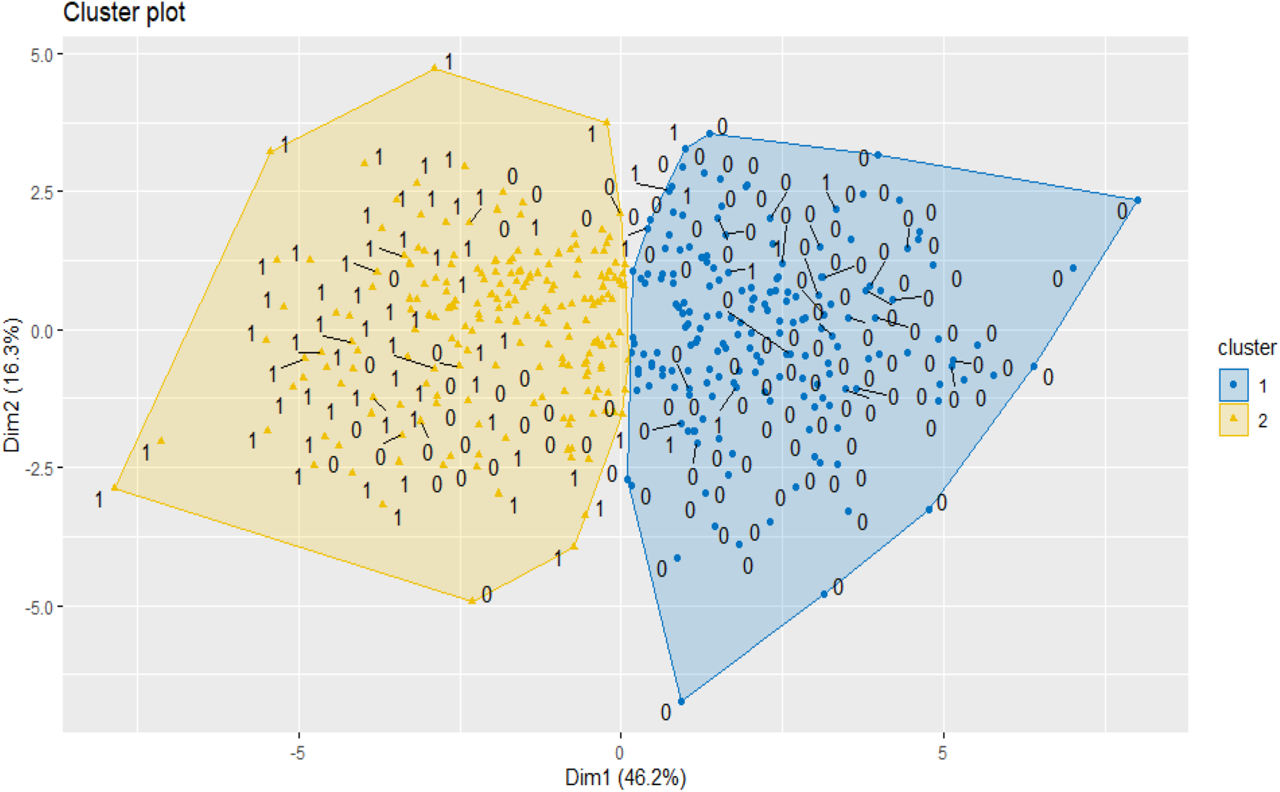
Cluster plot for clustering via k-means, for the playoffs.

Some standard measures to assess the effectiveness of clustering are the silhouette coefficient (SC), the adjusted Rand index (ARI) and the Dunn index (DI) For our data, the values of these indices were, respectively, 0.255, 0.817 and 0.081. Using the ARI our clustering appears to be quite good, but it is not effective according to the other two measures.

For the Final Four, we obtained the following results, using two clusters again. Among the 324 teams that did not qualify, 182 teams were in cluster 1 and 142 teams in cluster 2. Among the 72 teams that qualified, only 5 teams were in cluster 1 and the 67 remaining teams in cluster 2. The values of the evaluation measures (SC, ARI and DI), were, respectively, 0.272, 0.928 and 0.132; all three values are higher compared to the previous case. In summary, through all the clustering algorithms we performed, our data separated better into two groups. However, the overall performance of clustering seems to be rather poor compared to the other methods in this section.

Classification

Before applying the classification techniques, we split our data in a 70% - 30% ratio between training and testing sets. The first method we used was the Support Vector Machines (SVMs) algorithm. The basic idea is to find a hyperplane that separates elements of two classes in a high-dimensional space (Hastie et al., 2009). We used the Radial Basis Function (RBF) in our analysis, with the value for parameter γ (gamma) equal to 1.

From the confusion matrix (Table 7), we see that 65 observations were correctly placed as teams that did not qualify for the playoffs, and 28 as non-qualified. Further, our model incorrectly classified 11 teams that did not qualify and 15 teams that qualified. In total, the model classified correctly 78.2% of the observations.

Table 7.

Confusion matrix for SVMs.

	Confusion Matrix
	Prediction	Actual
	Prediction	0	1
Playoffs	0	65	15
Playoffs	1	11	28
Final Four	0	95	14
Final Four	1	2	8

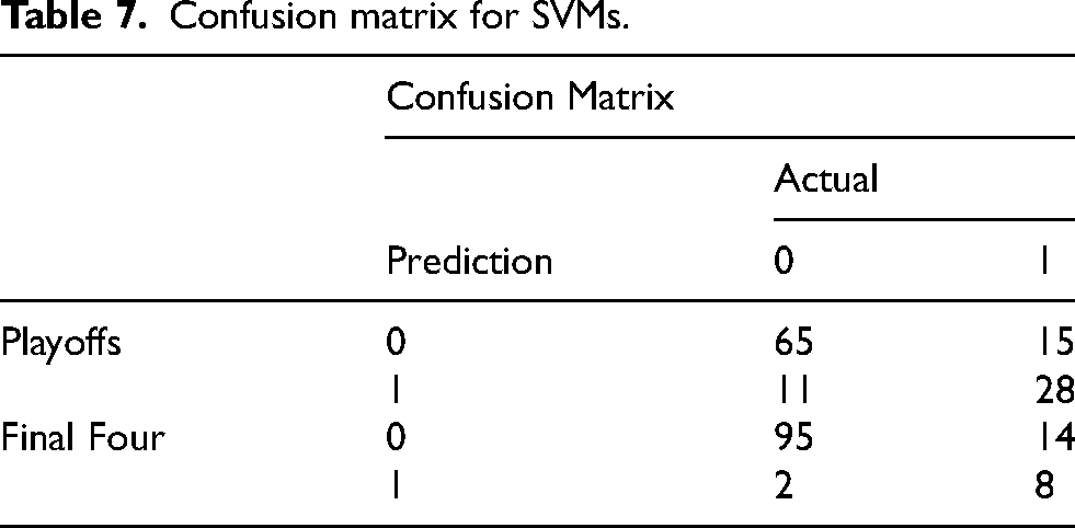
Following the same procedure for the Final Four phase, we found that 95 observations were correctly assigned to teams that did not qualify, and 8 to teams that qualified. The number of incorrect classifications were 14 for qualified teams and 2 for non-qualified. Thus, the model correctly classified 103 observations and only 16 incorrectly, based on the test set. Overall, a better classification seems to have been carried out for this phase (86.6% correct classifications).

The second method that we used for classification was the Random Forest algorithm, which has gained considerable attention in recent years because of its ability to handle complex classification problems (Breiman, 2001). The results were again better for the Final Four phase (99 correct classifications out of 119, i.e., a 83.2% percentage), while for the playoffs we had 76.5% correct classifications.

The effect of individual players

In this section we examine the effect that the top players have had, over the years, on the performance of their teams. In particular, we have carried out two analyses, denoted respectively by A and B below.

A: We calculated for each team, the averages of points and PIR of their five best players for each season. We wanted to study how these averages separated the teams, depending on whether they qualified for the playoffs and Final Four.

B: We singled out the top ten players in points and PIR per season, and looked at how many of them corresponded to teams that reached the playoffs, and teams that participated in the Final Four.

A. First we present boxplots for both points and PIR in order to see how the performance of the top players affected qualification to the playoffs (Figure 9) and the Final Four (Figure 10); on each graph, the boxplot on the right corresponds to teams which qualified.

Figure 9.

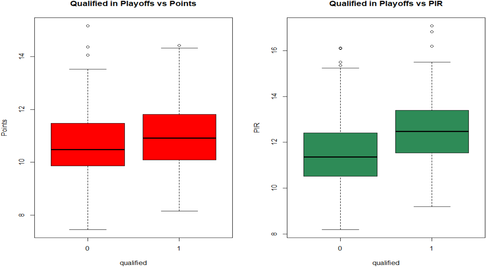
Boxplots for points and PIR, regarding qualification to playoffs.

Figure 10.

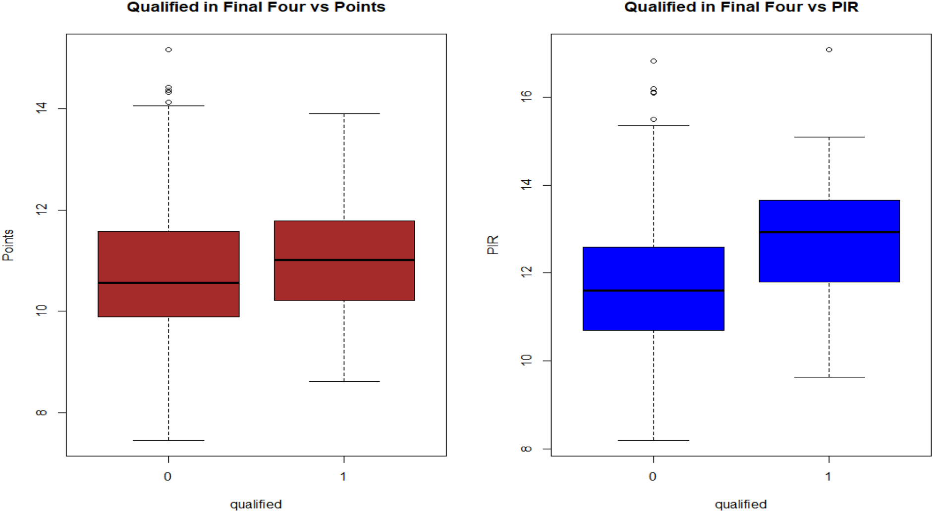
Boxplots for points and PIR, regarding qualification to final four.

As we can see from these boxplots, the median for the teams that qualified is higher than the one for the teams that did not qualify, both in terms of points and PIR. The differences are much more pronounced when considering the PIR rather than points. In particular, in both cases the median for qualified teams exceeds the third quartile of the average performance of the top players for non-qualified teams. There are a few values exceeding the upper threshold in the boxplots, both for points and the PIR values. There appears to be evidence for negative skewness in the points of the teams that did not qualify for the playoffs, and positive skewness in the PIR in the teams that qualified in the Final Four.

Looking at the means rather than the medians of these quantities, we performed t-tests to see if they differ. The average scoring, among the top 5 players for teams that qualified in the playoffs is $10.96 \pm 1.25$ , while for non-qualified teams it is $10.68 \pm 1.25$ ; their difference is significant (p = 0.033). Regarding qualification to the Final Four, the average scoring of the top 5 players is $10.95 \pm 1.13$ for qualified teams and $10.75 \pm 1.28$ for non-qualified; the difference is now non-significant (p = 0.196).

The average PIR, among the top 5 players for teams that qualified in the playoffs is $12.52 \pm 1.40$ , while for non-qualified teams it is $11.50 \pm 1.47$ ; their difference is highly significant (p < 0.0001). Regarding qualification to the Final Four, the average PIR of the top 5 players is $12.81 \pm 1.38$ for qualified teams and $11.68 \pm 1.49$ for non-qualified; the difference is significant (p < 0.0001) once again. In conclusion, it is not so much the scoring of the top players that discriminates qualified and non-qualified teams (esp. for the Final Four) but it is rather the overall performance of the top players that is affecting qualification.

B. For this part, we chose the top-10 players, according to PIR for each Euroleague season. Excluding the 2001–2004 and 2019–20 seasons, there are 180 player performances in total for the remaining 18 seasons; among them, 86 players played for teams that qualified for the playoffs, while 49 played in the Final Four. Indicatively, in Figures 11 (playoffs) and 3.12 (Final Four) we present violin plots for the points and PIR of these players. The distributions are now fairly similar in all cases, noting that violin plots for qualified teams are `fatter’, reflecting the fact that we have fewer observations and larger variance in this case.

Figure 11.

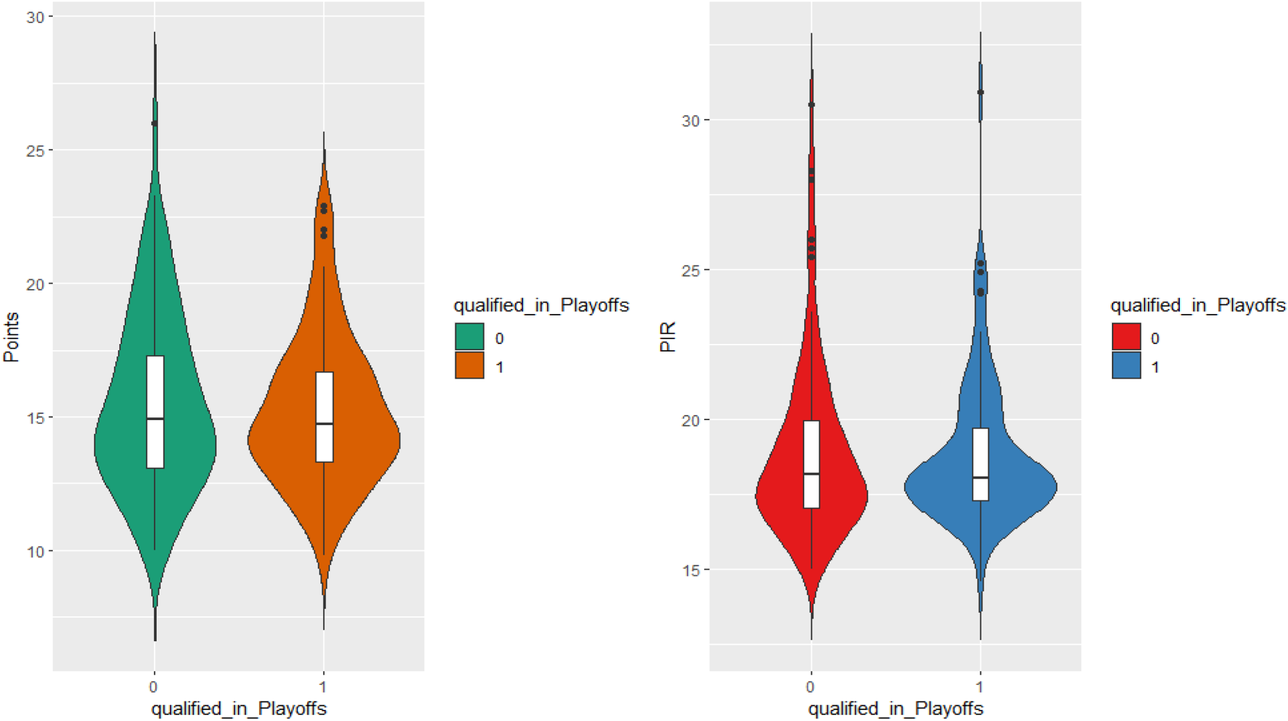
Violin plots for points and PIR, regarding qualification to playoffs.

In terms of points, the median for teams (of players) which did not qualify in the playoffs is higher than for teams that did, which is very interesting. The same is also true for Final Four participation, both for points and the PIR! The only case where the group of (players of) qualified teams had a higher median is the left plot of Figure 11, regarding the PIR and the playoff phase. Seven outliers (very high PIR scores) exist for players whose teams did not qualify, and four for those that did.

It appears that players with quite high performances, both in terms of points and PIR, correspond to teams that did not qualify in the two phases we examine. Thus it seems that for a team to qualify for the subsequent phases, it is not enough to have one player with a high PIR, but more players with a relatively good performance is much more needed (Figure 12).

Figure 12.

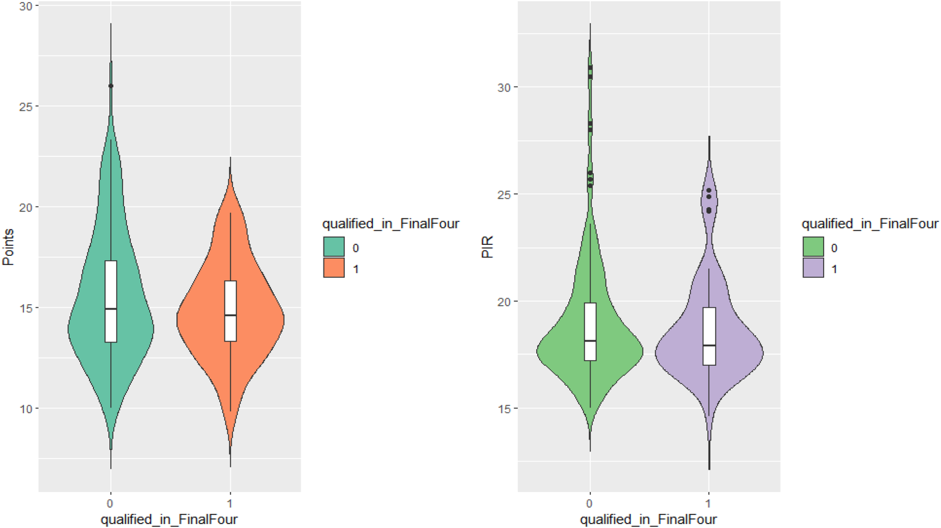
Violin plots for points and PIR, regarding participation in the final four.

Examining the equality of means, for the playoff phase neither the means of points (p = 0.514), nor the PIR (0.8092) are significantly different. The same conclusion can be drawn for the Final Four, as the p-value for the points is equal to 0.080 and for PIR it is 0.477.

Discussion

Studying how team statistics have varied through time, the most prominent changes seem to be a steady, substantial increase in FT% and assists and an (almost linear) decrease in the number of fouls. Through logistic regression, the model for the playoffs, which was found adequate, had PTSpPOS, DR, POS/G, FD, FT%, ORB% and STL as significant explanatory variables, while the corresponding model for the Final Four, which had a better performance, had eFG%, TR, PACE, FD, TO, STL and BLK. In general, teams that qualify for the playoffs perform better in nearly all boxscore statistics than non-qualified teams; this is reinforced by the machine learning feature selection algorithm, which identified a large number of variables affecting qualification to a later stage. In particular, and excluding PIR, points per possession and eFG% seem to be the most influential indicators for qualification to the playoffs and the Final Four, respectively. It is noticeable that, although points per game have a strong positive impact on a team's success, especially for playoff qualification, the number of possessions per game and pace have a negative impact. In addition, clustering algorithms consistently separated data into two groups. Both algorithms we used for classification gave better results for the Final Four (86.6% and 83.2% correct classifications, respectively) compared to playoff qualification.

Examining the impact of individual players, we observed that the overall performance of top players significantly contributed to team qualification, particularly for the Final Four. For teams that reached the Final Four stage, average scoring of their top 5 players does not differ from the top-5 player scoring in the remaining teams; considering their overall performance, however, as measured by the PIR, the associated difference is highly significant ( $p < 10^{- 4}) .$ Finally, and although over the years some very high annual player performances came from teams that did not reach the second phase of the competition, it is clear that teams require several players with relatively strong performances in order to qualify, rather than one player with a high PIR. Teams aiming for reaching far in the playoffs should prioritize assembling a roster with several key players rather than relying on a single standout player. In addition, since eFG%, STL, and BLK were significant for Final Four qualification, roster construction should ensure a balance between offensive efficiency and defensive ability.

Regarding the use of the PIR, which has often been criticized, we note the following. In our view, PIR is a valuable metric for assessing a player's overall contribution, as it aggregates key statistics into a single measure that provides practical insights into team performance. It has been argued that PIR fails to capture the true impact of players, due to a lack of appropriate weighting, such as adjustments for clutch situations or pace. Despite these limitations, our findings confirm its usefulness: Final Four teams consistently exhibit higher PIR across multiple players, highlighting the importance of balanced team contributions. While PIR does not account for pace, defensive skills, or role-specific nuances, its shortcomings are mitigated when it is used in conjunction with metrics such as eFG% and PTSpPOS. As such, PIR provides a strong basis for assessing team success, especially when integrated into a broader analytical framework.

The negative correlation between pace and possessions per game with qualification implies that more controlled plays improve the chances of a team's success. Head coaches could prioritize acquiring players who are comfortable in half-court systems and thrive in disciplined setups. Coaches should also focus on metrics like STL and BLK in defensive training, as they are significant for success at the Final Four phase. Moreover, our findings on eFG% and PTSpPOS stress that efficient scoring and intelligent shot selections are critical. Coaching stuffs could focus on training that improves shooting accuracy and decision-making. Finally, considering the importance of a balanced PIR, they might de-emphasize “hero ball” and promote systems that distribute offensive and defensive responsibilities across the roster.

Footnotes

ORCID iD

Konstadinos Politis

Funding

The authors received no financial support for the research, authorship, and/or publication of this article.

Declaration of conflicting interests

The authors declared no potential conflicts of interest with respect to the research, authorship, and/or publication of this article.

References

Akers

Wolff

Buttross

(1991) An empirical examination of the factors affecting the success of NCAA division I college basketball teams. The Journal of Business and Economic Studies 1: 57–71.

American Statistical Association (2017) Statistical Science Applied to Sports. In: Statistical Significance: Statistical Science Aiding Sports. Available at https://www.amstat.org/asa/files/pdfs/StatSig/StatSigSports.pdf

Breiman

(2001) Random forests. Machine Learning 45: 5–32.

Canuto

de Almeida

(2022) Determinants of basketball match outcome based on game-related statistics: A systematic review and meta-analysis. Eur J Hum Mov 48: 4–20.

Chernoff

(1973) The use of faces to represent points in k-dimensional space graphically. Journal of the American Statistical Association 68(342): 361–368.

Conover

(1999) Practical Nonparametric Statistics, 3rd ed New York: Wiley.

Cox

Snell

(1989) Analysis of Binary Data. 2nd ed. London: Chapman and Hall.

Csataljay

O’Donoghue

Hughes

, et al. (2009) Performance indicators that distinguish winning and losing teams in basketball. International Journal of Performance Analysis in Sport 9(1): 60–66.

de Rose

(2004) Statistical analysis of basketball performance indicators according to home/away games and winning and losing teams. J Hum Move Stu 47(4): 327–336.

10.

Dogan

Ersoz

(2019) The important game-related statistics for qualifying next rounds in euroleague. Montenegrin Journal of Sports Science and Medicine 8(1): 43–50.

11.

García

Ibáñez

De Santos

, et al. (2013) Identifying basketball performance indicators in regular season and playoff games. Journal of Human Kinetics 36(1): 161–168.

12.

Gómez

Lorenzo

Sampaio

, et al. (2008) Game-related statistics that discriminated winning and losing teams from the Spanish men’s professional basketball teams. Collegium Antropol 32(2): 315–319.

13.

Hastie

Friedman

Tisbshirani

(2009) The Elements of Statistical Learning: Data Mining, Inference, and Prediction. New York: Springer.

14.

Ibañez

Garcia-Rubio

Gómez

MÁ

, et al. (2018) The impact of rule modifications on elite basketball teams’ performance. Journal of Human Kinetics 64(1): 181–193.

15.

Ibañez

Sampaio

Feu

, et al. (2008) Basketball game-related statistics that discriminate between teams’ season-long success. European Journal of Sport Science 8(6): 369–372.

16.

Karipidis

Fotinakis

Taxildaris

, et al. (2001) Factors characterizing a successful performance in basketball. J Hum Mov Stu 14(5): 385–398.

17.

Kursa

Rudnicki

(2010) Feature selection with the Boruta Package. Journal of Statistical Software 36(11): 1–13.

18.

Kursa

Rudnicki

(2011) The all relevant feature selection using random forest arXiv preprint arXiv:1106.5112.

19.

Lorenzo

Gomez

Ortega

, et al. (2010) Game related statistics which discriminate between winning and losing under-16 male basketball games. J Sport Sci Med 9: 664–668.

20.

Mandić

Jakovljevic

Erculj

, et al. (2019) Trends in NBA and Euroleague Basketball: Analysis and comparison of statistical data from 2000 to 2017. Plos One 14(10): 1–17.

21.

Marmarinos

Apostolidis

Bolatoglou

, et al. (2016) Game-related statistics that discriminate playoffs teams from the rest of the competition in Euroleague Basketball. Journal of Athletic Enhancement 5: 6. of 5, 2.

22.

Mikołajec

Banyś

Żurowska-Cegielska

, et al. (2021) How to win the basketball Euroleague? Game performance determining sports results during 2003–2016 matches. Journal of Human Kinetics 77: 287–296.

23.

Senaviratna

Cooray

TMA

(2019) Diagnosing multicollinearity of logistic regression model. Asian Journal of Probability and Statistics 4(2): 1–9.

24.

Štrumbelj

Vračar

Robnik-Šikonja

, et al. (2013) A decade of euroleague basketball: An analysis of trends and recent rule change effects. Journal of Human Kinetics 38: 183–189.

25.

Tan

P-N

Steinbach

Karpatne

, et al. (2018) Introduction to Data Mining, 2nd edn. Boston, MA: Pearson Education.

26.

Tsamourtzis

Salonikidis