Sage Journals: Discover world-class research

Abstract

The central subject of this study is to examine the applicability of Pythagorean Expectation (PE) formula (introduced by Bill James) on basketball EuroLeague data. A secondary aim is to identify the optimal value of the main turning parameter of this method based on EuroLeague data. The data of our study are composed of boxscore statistics of EuroLeague games for seasons from 2016–2017 to 2019–2020 (four seasons in total). By applying the PE model on EuroLeague data, the main conclusion is that the method predicts the final standings for 2019–20 season with accuracy comparable with other, more sophisticative, predictive methods such as logistic regression models using box-score statistics evaluated at the end of each game. Bootstrap was used to obtain confidence intervals of the PE main parameter. The estimated exponent parameter was found to range between 9.98 and 12.32 with 95% confidence (point estimate equal to 11.19). This is the first study which provides accurate (point and interval) estimation of the PE using EuroLeague Basketball data.

Keywords

pythagorean expectation prediction basketball euroleague bootstrap estimation of exponent

Introduction

The sports betting industry, which is worth billions of dollars, largely relies on the fact that predicting the result of a sporting event is challenging. Although a large amount of data and sports related information is easily accessible and available nowadays, prediction of the final league table is still difficult. Nevertheless, the games in major leagues have become more predictable over the last two decades due to the increased data information and the advanced statistical and machine learning methods used for prediction. Such predictive methods in basketball can be beneficial for multiple individuals and companies involved in the sport including betting companies and team managers (regarding team management and planning); see for details in Li and Xu (2021).

One of the earliest attempts to predict basketball game outcomes was by Schwertman et al. (1991). They developed models to estimate the probability of each seed winning a regional tournament. In the following, we report selected studies on predictive basketball modeling, including their accuracy measures in order to have a picture of their efficiency. Hu and Zidek (2004) predicted the NBA final series outcome of the ‘96–‘97 season using a weighted likelihood method and team-level boxscore statistics as features. They analyze match history to assess each team's chance of winning individual games, ultimately forecasting a Bulls championship with probabilities from 61% to 71%, aligning with the actual outcome.

Regarding machine learning techniques, Loeffelholz et al. (2009), examined the success of basketball teams in the NBA with the use of neural networks as a tool such as feed-forward, radial basis, probabilistic and generalized regression neural networks. Boxscores statistics of 620 NBA games were collected and used to train the abovementioned neural networks resulting in a 74% accuracy on average to predict the winning team. This study aimed to achieve a higher prediction rate compared to predictions made by numerous experts in the field of basketball (68% approximately).

Several predictive models utilize team-level boxscore statistics as explanatory features, such as total points scored or average rebounds per game. Cao (2012), for example, used team-level boxscore statistics to predict NBA game outcomes with logistic regression, Naïve Bayes, SVM, and ANNs, reporting accuracies between 66% (Naïve Bayes) and 68% (logistic regression). Similarly, Beckler et al. (2013) used team-based NBA player stats from the ‘91–‘92 to ‘96–‘97 seasons. Applying linear regression, logistic regression, support vector machines (SVM), and artificial neural networks (ANNs), they achieved a 70% accuracy with linear regression. ANNs, however, performed the worst, with a 65% accuracy rate. The authors also noted that some seasons had lower model performance, suggesting increased variability during those periods. Finally, Tzai et al. (2023) implemented logistic regression, random forrest, XG-boost and ensemble learning in Euroleague, Eurocup, the Greek and the Spanish national leagues reporting accuracy up to 78% for the Greek league using ensemble learning or logistic regression (normal season) and up to 87.5% for the random forest implemented in Eurocup data. The results of these three studies are in close agreement with each other, as well as with findings from other research articles and expert prediction rates.

This short review is by no means exhaustive, and it only aims to provide some indicative works on the topic; for a more thorough review see in Tzai et al. (2023) and references therein.

In this work, we study the implementation of the Pythagorean expectation (PE) method in Euroleague basketball data. PE was introduced in sabermetrics (Baseball statistics) as an intuitive method of team evaluation by James (1980). Sabermetrics is the empirical analysis of baseball, especially baseball statistics that measure in-game activity¹ and it was one of the first areas where sports analytics were used widely. Similarly, advanced statistics in Basketball are used by a large number of modern basketball analysts today. Such advanced statistics are known as APBRmetrics (the acronym APBR stands for the Association for Professional Basketball Research)².

One of the statistical innovations, attributable to James (1980) when he introduced sabermetrics, is the PE which is a formula for estimating the percentage of games a team should have won based on the number of runs they scored³ and allowed⁴. In baseball, the PE formula is given by the following equation:

P y t h a g o r e a n W % = \frac{R u n s S c o r e d^{x}}{R u n s S c o r e d^{x} + R u n s A l l o w e d^{x}} .

(1)

In the initial introduction of the formula, the exponent x was set equal to the value of two (2) for baseball. Since then, it has been modified to 1.82, instead of two, which slightly improves the “fit” in terms of accuracy (Davenport & Woolner, 1999). Rothman (2014) suggested that the exponent in the PE should range from 1.75 to 2.05 for baseball. Miller (2007) proposed a similar range of values (1.82–2). Similar values (1.92 and ∼2.0) were also suggested for ice hockey by Cochran and Blackstock (2009) and Dayaratna and Miller (2012), respectively. The PE was also implemented in other sports as well, such as football and basketball. For example, Morey (2003) applied PE to professional football reporting as the optimal value for the exponent to be equal to 2.37. In basketball, the exponent was found to be much higher with values ranging from 13.91 to 16.5.

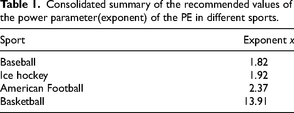
Specifically, Oliver (2004) suggested the value of 14 using basketball ΝΒΑ data. Similar was the value (13.91) that Morey (2003) found as the optimal one using data of three ΝΒΑ seasons (1990–91 to 1993–94). A few years later, Oliver agreed in the use of an exponent of 16.5 for the analysis of 2006–7 NBA data according to Kubatko et al. (2007). However, Kubatko et al. (2007) conducted a more detailed analysis of NBA data from the 1940s. In this study, he examined how the exponent changed across different decades. He found that the value of 16.5 was not optimal (in terms of RMSE) for any of the decades under investigation. Thus, he returned to the original value of 14 proposed by Oliver (2004) claiming that it was more appropriate for the more recent basketball data he analysed; for more details, see Chen and Li (2016) and Kaplan and Rich (2017). Table 1 presents a summary of the recommended values of exponent x for different sports.

Table 1.

Consolidated summary of the recommended values of the power parameter(exponent) of the PE in different sports.

Sport	Exponent x
Baseball	1.82
Ice hockey	1.92
American Football	2.37
Basketball	13.91

By comparing the actual and Pythagorean winning percentages, one can estimate and predict whether a team is over-performing or under-performing. In other words, Pythagorean Winning Percentage provides a better indication of how well a team is playing. Of course, for this statistic to be reliable, a large enough sample of games is required.

In addition to the most popular approaches of Oliver (2004), Morey (2003) and Kubatko et al. (2007) implemented in NBA as already discussed, Rosenfeld et al. (2010) used data from 14 more recent seasons and found the optimal value to be 14.05.

Chen and Li (2016) investigated the accuracy of the formula on the NBA by using data from seasons 1994 to 2014. As response variable (predictor), they used the ratio of Points Scored and Points Allowed, called PtR. Their findings confirmed that the exponent value is slightly above 14.

To illustrate this, they calculated a measure of the shrinkage phenomenon in a prediction (out-of-sample) scenario. To do so, they used a shrinkage factor defined as: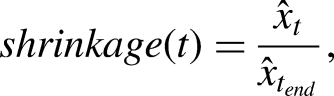

s h r i n k a g e (t) = \frac{{\hat{x}}_{t}}{{\hat{x}}_{t_{e n d}}},

where

{\hat{x}}_{t}

and

{\hat{x}}_{t_{e n d}}

are the estimated exponent values at a time t and at the end of the season (denoted by

t_{e n d}

), respectively.

It has been proven that this shrinkage factor varies from 0.5 early in the season to nearly one towards the end of the season. This value increases over time since fewer games remain to be played in the future as time progresses toward the end of a season.

Although there are many studies for basketball, only a few of them are oriented to the analysis of EuroLeague data (Giasemidis, 2020). Additionally, in basketball studies, it is important to keep in mind that results obtained with NBA data are not always immediately generalizable to Europe (Zuccolotto and Manisera, 2020). Thus, one of the goals of this study is to define the value of the PE exponent for EuroLeague basketball games.

In this study, we employed data from four different EuroLeague seasons (2016–17 to 2019–20). The optimal exponent value was estimated using the first three seasons as a training dataset and afterwards, this value was used for the implementation in the test dataset (2019–20). Further information about the data structure of this study is included in Section 2.

In basketball, the PE win/loss formula is based on points scored and points allowed by the home team. However, these variables are available only after the end of the game. Thus, it is more of an explanatory formula that indicates whether a team has overachieved or underachieved the expected performance of that year according to our fitted PE model.

Nevertheless, Baysal and Yildiztepe (2019) provide a way of explaining how to use PE for prediction. In their work, they explicitly state that: “PE is typically used in the middle of a season to predict the standings for the end of a season. For example, if a team wins more than the predicted in the halfway through a season, analysts claim that the team will complete the remaining half of the season with fewer winnings than the predicted.”. Miller (2007) also agreed with this approach.

In this study, our approach will be based on this predictive perspective of the PE formula. More specifically, we will focus on the prediction of the number of wins each team will have halfway through the season based on the PE formula. The total number of projected wins will be compared with the actual wins of each team to examine whether the PE formula accurately predicts the season final rankings based on wins. To achieve this, and before proceeding to the implementation of this predictive approach, it is important to estimate the exponent x of the PE formula.

The rest of the paper is structured as following. Section 2 presents the details of the dataset of our study. Section 3 focuses on a thorough study regarding the estimated value of the exponent parameter including bootstrap confidence intervals. In Section 4 we present the results of the study regarding the predictive ability of PE. The paper concludes with a discussion (Section 5).

Dataset of the study

The data structure, in this study, was produced by the developers of newstats.com. The raw data are in the form of boxscore statistics for every single game (both for every player and team) that took place in the EuroLeague from the season 2016–2017 to 2019–2020.

The data were initially provided in a JSON file type and then were imported and analysed in R (version 4.1.3; R Core Team, 2023). The dataset includes both regular season games and playoff games from season 2016–17 to 2019–20 (4 seasons in total). For seasons 2016–17, 2017–18 and 2018–19, sixteen (16) teams participated and competed with each other, whereas the total number of teams in the EuroLeague 2019–20 was increased to eighteen (18).

Season 2019–20 was incomplete due to Covid-19 pandemic. Specifically, the last six (6) fixtures of the regular season and the playoff games were cancelled. Therefore, no winner was announced for this season. To implement our PE method, we decided to create a balanced dataset for season 2019–20 by using a subset of it. This subset considered only the 11 games for each team from the first half of the regular season (fixtures 1–17) that also took place in the second half season (fixtures 18–28). For example, the game Panathinaikos OPAP – ALBA Berlin that took place in Fixture 8 was not included in this balanced dataset since the return match between those two teams never took place due to the pandemic. Thus, the total games for each team is twenty-two (22) while the total sample size of this balanced dataset is 198 games.

Statistical analysis

First, we focus on the estimation of the exponent values for each season in our dataset. Our objective is to get the optimal exponent value that produces the lowest Root Mean Square Error (RMSE) between the anticipated and actual wins. According to its mathematical definition, RMSE is given by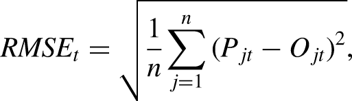

R M S E_{t} = \sqrt{\frac{1}{n} \sum_{j = 1}^{n} {(P_{j t} - O_{j t})}^{2}},

where j is an index which runs over all n teams competing in a league, t specifies the time where the RMSE is calculated,

P_{j}

is the estimated number of wins of Team j under the PE approach at time t while

O_{j}

is the observed number of wins for Team j at time t.

At half season, we have estimated the optimal exponent value by minimizing the RMSE over the first-half season data (in-sample RMSE). Next, we applied the Pythagorean formula using the half-season exponent value to predict how many wins each team are expected to have. This projected number of wins was added to the actual wins of each team. Then this number was compared with the number of actual wins at the end of the season and the respective RMSE value was computed. Hence the RMSE at the end of the season is the out-of-sample RMSE which tests the performance of the method in the second half of the season which was used as a test dataset. Finally, we computed the Pearson correlation coefficient between the predicted wins and actual wins at the end of each season. All correlations were found to be statistically significant (p-value < .01).

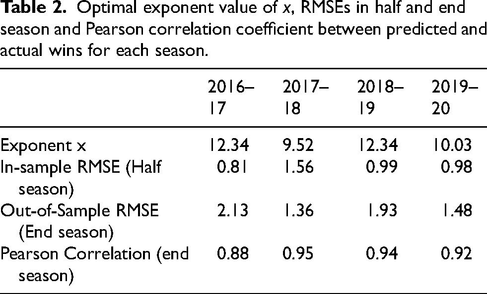
The exponent value ranged from 9.52 to 12.34, with the smallest value identified in 2018–19 and the greatest in seasons 2016–17 and 2018–19 (see Table 2). Remarkably, for two distinct seasons the optimal exponent value was found to be equal to 12.34, and the half-season RMSE values, although not the same, are quite close (0.81 for the 2016–17 season and 0.99 for the 2018–19 season). However, the lowest RMSE value at the end of the season was identified in 2017–18 (with a value equal to 1.36). It is noteworthy that, for 2017–18, we had the worst RMSE value in the half of the season and the best one at its end.

Table 2.

Optimal exponent value of x, RMSEs in half and end season and Pearson correlation coefficient between predicted and actual wins for each season.

	2016–17	2017–18	2018–19	2019–20
Exponent x	12.34	9.52	12.34	10.03
In-sample RMSE (Half season)	0.81	1.56	0.99	0.98
Out-of-Sample RMSE (End season)	2.13	1.36	1.93	1.48
Pearson Correlation (end season)	0.88	0.95	0.94	0.92

Next, we proceed with the evaluation of the PE formula when used as a prediction model. This model was used to predict the final standing of a given season based on the games that took place in the first half of a season. In this way, we obtain good proxies of the performance of each team based on the points of the first half season. Nevertheless, for the computation of the exponent used in the PE formula, we have used the previous three seasons (2016–19) in order to get a more precise and reliable estimate of this quantity of primary interest.

To obtain the estimate of the exponent, we have applied a straightforward greedy search algorithm assessing the RMSE values for a range of exponent values in the interval [2,30]. The optimal value of the exponent ( $\hat{x}$ ) using the data of all seasons was found to be equal to 11.19, with RMSE = 1.71 in the train dataset (seasons 2016–19). This value is then used in the PE formula to predict the final ranking of season 2019–20 after considering the points and the results of the first half season of 2019–20.

However, before proceeding to the implementation of this PE formula, we have also estimated the 95% confidence interval of the exponent via bootstrap. Bootstrap is a statistical method for inference about a population measure using sample data which was developed by Efron; see for details in Efron and Tibshirani (1994). By this method, we can estimate the confidence interval (CI) by drawing samples with replacement from the sampled dataset. For each re-sampled dataset, we obtain an estimate of the parameter of interest (here the exponent). At the end, the output of bootstrap will be a sample of the parameter of interest and from this sample, we can obtain confidence intervals (for example using simply the quantiles of the sample) or other more demanding quantities.

Due to its ease of implementation, this approach is frequently used to obtain estimates of confidence intervals for complicated estimators. Furthermore, bootstrapping is an inexpensive technique to repeat the experiment and obtain additional sample data sets, as well as a suitable means of controlling and verifying the stability of results. Additionally, bootstrapping is an appropriate way to control and check the stability of our estimated parameter of interest, and its computational cost is reasonable in comparison to other simulation-based methods.

In the following, we provide a bootstrap-based 95% confidence interval (CI) using bootstrap samples ${\hat{x}}^{(t)}$ for t = 1,…, T for T = 1000 sample replicates. We have consider all seasons as input for the bootstrap method.

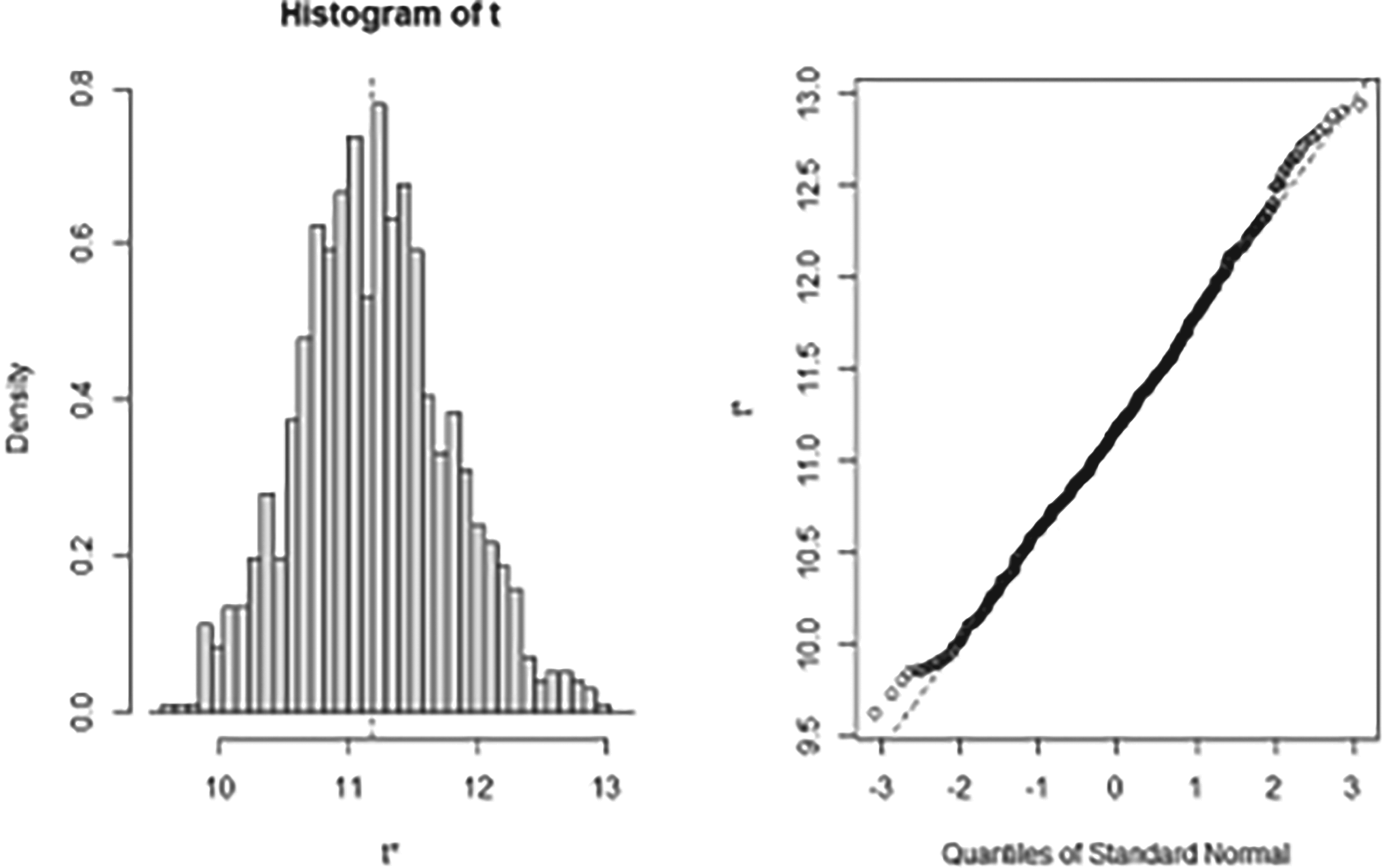
Figure 1 presents the generated histogram (on the left) and the corresponding qqplot (on the right) of the bootstrap replicates ( ${\hat{x}}^{(t)}$ for t = 1,…, T) for which the distribution seems to be close to the normal one.

Figure 1.

The estimated distribution (histogram and QQ plot) of the exponent (x) generated using bootstrap samples.

Regarding the results, the following four methods of the boot package (in R) were implemented to obtain the resulting confidence intervals.

Normal bootstrap which uses the estimated bootstrap-based standard error of ( $\hat{x}$ ) for the calculation of the CI.

Basic bootstrap that calculates the upper and lower limit of estimator.

Percentile bootstrap uses percentiles/quantiles to calculate the CI.

Bias Corrected Accelerated (BCa) bootstrap uses the percentiles from the bootstrap samples after correcting for bias correction and skewness of the distribution.

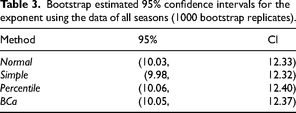
Results from these four methods are given in Table 3. All methods provide similar intervals recommending that x will vary from 10 to 12.40 with 95% confidence.

Table 3.

Bootstrap estimated 95% confidence intervals for the exponent using the data of all seasons (1000 bootstrap replicates).

Method	95%	CI
Normal	(10.03,	12.33)
Simple	(9.98,	12.32)
Percentile	(10.06,	12.40)
BCa	(10.05,	12.37)

Given that the PE technique is the main focus of our study, it is imperative to examine its main variables of interest, namely the points scored by the home team and the points scored by the away team (or the points permitted by the home team). Since in our study, we used only boxscore information rather than play-by-play statistics, we extracted the final score of each game, including any overtime.

Thus, on average, the home team scores 82 points and concedes 77 points in a typical Euro League game for the seasons under investigation. Given that the exponent value, as previously determined, is equal to 11.19, then the predicted winning percentage is found to be about 0.67. In other words, the home team is expected to win two out of three (2/3) games, based on PE formula for this value of the exponent parameter.

The exponent value of 11.19 found in EuroLeague, is quite smaller than the reported values in NBA studies where it ranges from 14 to 16.5 (Oliver 2004, and Kubatko et al., 2007). Moreover, this figure is also smaller than the corresponding one obtained using NBA data (for the period 2015–19) assuming the same win margin of 0.67 (as in the EuroLeague) which is found equal to 13.

Results

Based on the exponent value x estimated in Section 3, we applied the PE formula to assess the fit of the approach by calculating the expected wins for each team in the first half of the 2019–20 season (in-sample evaluation). Overall, the PE managed to reduce uncertainty by 77% in comparison to using just the overall mean (i.e., the constant model); Pearson correlation 0.88. The corresponding RMSE is equal to one unit which means that the error in the expected wins will be about one game; see at the Appendix. According to PE, CSKA Moscow was expected to win about eight (8.15) out of the eleven games they played in the first half of the season. However, CSKA won only seven games. As a result, CSKA underachieved according to what was expected by PE. Conversely, ASVEL has won five games when they should have only won roughly three (3.22) according to PE. Thus, they exceeded expectations by two games based on PE model.

Next, we predict the final rankings based on the predicted wins of the second half of the season. The final predicted wins at the end of the season for each team, are calculated as the sum of the actual wins at the half-season and the projected wins at the second half of the season; see at the Appendix and Figures 2 and 3 for the comparison between predicted and actual wins for all four seasons under consideration. The RMSE value obtained with this approach at the end of the season, is equal to 1.50, while the Pearson correlation between predicted and actual wins is found to be equal to 0.93.

Figure 2.

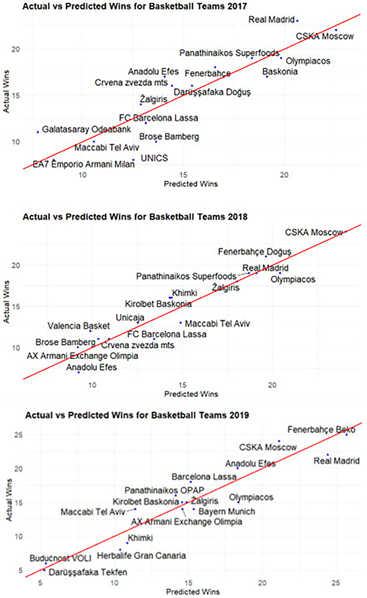
Predicted vs actual wins for each team in each season of the train dataset for seasons 2017–19 (out-of-sample evaluation). (a) Season 2017–18, (b) Season 2018–19, (c) Season 2019–20.

Figure 3.

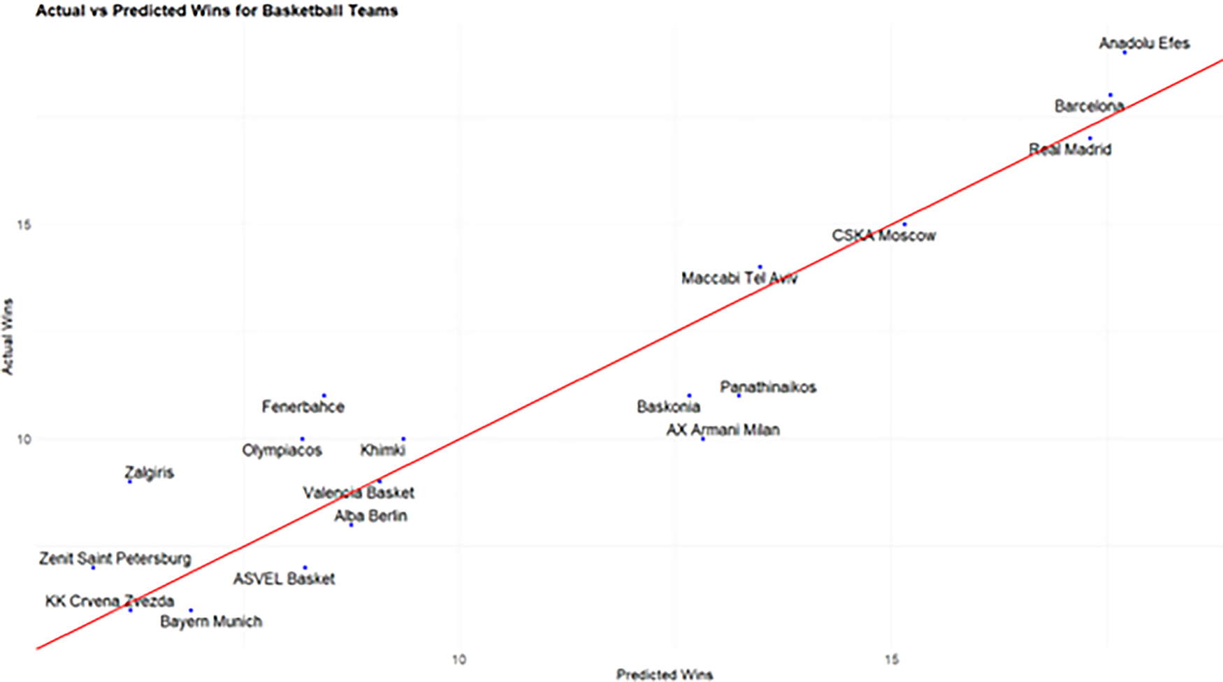
Predicted vs actual wins for each team for season 2019–20 (out-of-sample evaluation).

Following a referee's comment, we also ran a logistic regression at the game level, using boxscore data at the end of each game as covariates. The resulting RMSE was 1.99, slightly higher than PE, and the Pearson correlation between predicted and actual wins was 0.86. The model predictions for Zalgiris, AX Armani Milan Panathinaikos and Fenerbahce are less accurate than for the rest of the teams with a difference of two or three games from the actual outcomes. For the rest of the teams, wins are predicted with higher accuracy, with a difference of less than two games from the actual results.

Discussion

This study focuses on the practical usefulness of the PE model for EuroLeague analysts, offering a simple yet effective tool for forecasting and decision-making. Overall, the findings of this study suggest that the PE approach provides sufficiently accurate predictions for EuroLeague basketball final league ranking.

The estimated exponent was found to be approximately equal to 11 in contrast to the corresponding value of 14 which is most commonly used in NBA data. This is the first study, in our knowledge, that produces (bootstrap) confidence interval for the EuroLeague exponent. All implemented methods indicate that the exponent varies between 10.03 and 12.33 with 95% confidence which seems to be systematically lower than the values found in NBA studies ranging from 13.91 to 16.5. Overall, the EuroLeague estimated exponent is notably lower, indicating a different dynamic in team performance prediction between the two leagues.

The optimal exponent value (11.19) identified in our study is lower than those reported in existing studies on Pythagorean expectation (14–16.5). However, those studies were based on NBA data, where each team plays considerably higher number of regular-season games than EuroLeague teams (82 games for NBA teams versus 30 for EuroLeague teams). Additionally, NBA games generally end up with higher scores than EuroLeague games, partly due to the NBA's longer game duration (eight additional minutes). The EuroLeague also places a stronger emphasis on defense, with the average points scored per team around 80 (vs. about 111 for NBA).

According to our findings, we believe that the PE model, implemented in this study, sufficiently forecasts the number of wins with the precision of about one or 1.5 games in in-sample and out-of-sample analysis. Moreover, in the out-of-sample analysis, the correlation between the predicted and observed wins in the final league table was high, ranging from 0.88 to 0.95 for seasons 2016–2020. The fact that PE may produce sufficiently accurate results by utilizing only the points scored and allowed in a subset of games during the season—in his case, half of the season—is rather remarkable.

In our study using Pythagorean Expectation to predict the final EuroLeague standings for the 2020 season, we evaluated the model's performance using Root Mean Squared Error (RMSE) and Pearson correlation between actual and predicted wins. The resulting RMSE of 1.50 and Pearson correlation of 93% demonstrate a strong alignment between predicted and actual wins, indicating a high level of accuracy in comparison to other methods.

Team and sports analytics experts may find this algorithm quite helpful due to its simplicity, as they may easily quantify expected team performance and use the results to determine whether their teams require any improvements. The PE formula can also be used to evaluate the individual contribution of each player (Hakes and Sauer, 2006). By using PE in player performance evaluation, we may quantify about each player's role in the team's winning percentage and gain insight about the importance of each player. Nevertheless, such an approach will not take into consideration the defensive contribution of basketball players which in European basketball is extremely important. Alternative approaches might be investigated in the future by implementing a similar approach not only to points but also to other (defensive or less direct) team and player statistics.

One of the main limitations of the Pythagorean Expectation model, as applied to predicting team performance in a league, is that it does not account for the interdependency of game outcomes among teams. Specifically, the model operates independently for each team, estimating the number of wins based on their scoring and defensive records without enforcing a constraint that the sum of all teams’ expected wins equals the total number of games played. As a result, it is possible for the predicted number of wins across teams to exceed the total number of available wins in the league, which reflects an inherent simplification of the model. This limitation stems from the model's focus on individual team performance metrics (points scored and allowed) rather than the broader competitive dynamics between teams.

Finally, when it comes to extensions of this study, the PE is based on a single-parameter function. Different approaches have been performed in other studies as well. Heumann (2016) introduced a new statistic, called “Pairwise” Pythagorean wins, which demonstrated, over 30-year dataset, to have a smaller overall root mean square error than the original Pythagorean formula.

In our study, we used the traditional formula of PE as it was introduced by Bill James (1980). Nonetheless, by extending or modifying the original formula to achieve greater generality, some recent studies have demonstrated that overall prediction accuracy can be considerably improved (Baysal and Yildiztepe, 2019).

Footnotes

Funding

The authors received no financial support for the research, authorship, and/or publication of this article.

Declaration of conflicting interests

The authors declared no potential conflicts of interest with respect to the research, authorship, and/or publication of this article.

Notes

Appendix

See Tables 4 and 5.

References

Baysal

Yildiztepe

(2019) Prediction of season-end point for football using pythagorean expectation. Journal of New Theory 27: 63–73.

Beckler

Wang

Papamichael

(2013) NBA Oracle. Zuletzt Besucht Am 1: 15213.

Cao

(2012) Sports data mining technology used in basketball outcome prediction . MSc Dissertation, Technological University Dublin.

Chen

(2016) The shrinkage of the pythagorean exponents. Journal of Sports Analytics 2: 37–48.

Cochran

Blackstock

(2009) Pythagoras and the national hockey league. Journal of Quantitative Analysis in Sports 5(2): 1–13.

Davenport

Woolner

(1999) Revisiting the Pythagorean Theorem: Putting Bill James’ Pythagorean Theorem to the Test. Baseball Prospectus, URL: https://www.baseballprospectus.com/news/article/342/revisiting-the-pythagorean-theorem-putting-bill-james-pythagorean-theorem-to-the-test/

Dayaratna

Miller

(2012) The pythagorean won-loss formula and hockey: A statistical justification for using the classic baseball formula as an evaluative tool in hockey. The Hockey Research Journal 2012/13: 193–209.

Efron

Tibshirani

(1994) An Introduction to the Bootstrap. 1st ed. New York: Chapman and Hall/CRC.

Giasemidis

(2020) Descriptive and Predictive Analysis of EuroLeague Basketball Games and the Wisdom of Basketball Crowds, arXiv:2002.08465.

10.

Hakes

Sauer

(2006) An economic evaluation of the moneyball hypothesis. Journal of Economic Perspectives 20(3): 173–186.

11.

Heumann

(2016) An improvement to the baseball statistic “pythagorean wins”. Journal of Sports Analytics 2: 49–59.

12.

F-F

Zidek

(2004) Forecasting NBA basketball playoff outcomes using the weighted likelihood. Lecture Notes-Monograph Series 45: 385–395.

13.

James

(1980) Baseball Abstract. Lawrence, KS: Manuscript.

14.

Kaplan

Rich

(2017) Decomposing pythagoras. Journal of Quantitative Analysis in Sports 13(4): 141–149.

15.

Kubatko

Oliver

Pelton

, et al. (2007) A starting point for analyzing basketball statistics. Journal of Quantitative Analysis in Sports 3(3): 1–22.

16.

(2021) Application of artificial intelligence in basketball sport. Journal of Education, Health and Sport 11(7): 54–67.

17.

Loeffelholz

Bednar

Bauer

(2009) Predicting NBA games using neural networks. Journal of Quantitative Analysis in Sports 5(1): 1–15.

18.

Miller

(2007) A derivation of the pythagorean won-loss formula in baseball. Chance Magazine 20: 40–48.

19.

Morey

(2003) STATS basketball scoreboard. In: Dewan

Sminda

(eds) STATS Basketball Scoreboard. New York: STATS, Inc.

20.

Oliver

(2004) Basketball on Paper: Rules and Tools for Performance Analysis. Washington, D.C., USA: Potomac Books Inc.

21.

R Core Team (2023) R: A Language and Environment for Statistical Computing. Vienna, Austria: R Foundation for Statistical Computing. https://www.R-project.org/

22.

Rosenfeld

Fisher

Adler

, et al. (2010) Predicting overtime with the pythagorean formula. Journal of Quantitative Analysis in Sports 6(2): 1–19.

23.

Rothman

(2014) A new formula to predict a team's winning percentage. The Baseball Research Journal 43(2): 97–105.

24.

Schwertman

McCready

Howard

(1991) Probability models for the NCAA regional basketball tournaments, The American Statistician 45(1): 35–38.

25.

Tzai

Ntzoufras

Vassalos

, et al. (2023) Predictions of European basketball match results with machine learning algorithms. Journal of Sports Analytics 9: 171–190.

26.

Zuccolotto

Manisera

(2020) Basketball Data Science: With Applications in R. Boca Raton, FL: CRC Press Taylor & Francis Group.