Sage Journals: Discover world-class research

Abstract

This paper evaluates the effectiveness of timeouts in the EuroLeague using Play-by-Play data to estimate short-run within-game effects and Box-Score data to assess season-level outcomes over the 2021–22 to 2023–24 regular seasons. Within games, timeout effectiveness is identified using an event-study framework comparing team performance in fixed possession windows immediately before and after each timeout, complemented by a difference-in-differences strategy exploiting situations in which teams are unable to call additional timeouts. Performance is measured by the point differential (points scored minus points conceded) over these windows. Under the identifying assumption that pre-timeout trends are comparable across treated and control situations, timeouts are associated with a statistically significant short-run improvement: the average point differential increases from $- 3.74$ before a timeout to $- 1.20$ afterward. Although economically meaningful in reducing opponent scoring runs by approximately 2.5 points on average, the post-timeout differential remains negative, indicating that timeouts primarily stabilize performance rather than reverse game momentum. To assess whether these short-run effects translate into sustained success, we extend the standard Four-Factor Model of Wins with a fifth factor capturing team-level timeout effectiveness. This additional factor provides no incremental explanatory power. From a coaching perspective, timeouts appear to function as short-term damage-control devices but do not systematically affect season-long competitive outcomes.

Keywords

Basketball analytics box-score data difference-in-differences EuroLeague play-by-play data timeouts

Introduction

Timeouts are a central coaching instrument in basketball, used to interrupt play, adjust tactics, and potentially influence short-run performance dynamics. Despite their strategic importance, empirical evidence on the effectiveness of timeouts remains mixed, particularly regarding whether they can alter in-game momentum or generate persistent performance gains. This paper evaluates the effectiveness of timeouts along two dimensions: their short-run impact on within-game performance and their longer-run implications for team success over an entire season. We define momentum as a short-run deviation in the scoring process from a team’s recent scoring baseline. Operationally, momentum is captured by sustained positive or negative scoring differentials over consecutive possessions, which we measure through (i) uncontested scoring runs and (ii) changes in the local point differential within fixed one-minute windows. Under this definition, a team is said to experience negative momentum when it concedes a sequence of points without response, generating a locally negative scoring differential relative to its recent performance.

This definition allows us to treat momentum as an observable feature of the scoring process rather than as a purely psychological construct. Timeouts are therefore interpreted as interventions aimed at altering the short-run conditional expectation of the point differential. The empirical question becomes whether, conditional on pre-timeout dynamics, the scoring process exhibits a statistically significant shift in its conditional mean following a timeout call.¹

From a theoretical perspective, timeouts may affect short-run performance through several non-mutually exclusive channels: (i) tactical adjustments that alter shot selection or defensive schemes, (ii) substitution patterns that modify lineup efficiency, and (iii) psychological interruption of opponent scoring sequences. In reduced-form terms, these mechanisms imply a shift in the conditional mean of the scoring differential immediately after the timeout. Our baseline empirical strategy does not separately identify these channels; instead, it estimates their combined effect on the local scoring process.² This conceptual framework aligns directly with our empirical design, which focuses on local changes in scoring performance in narrowly defined windows around timeout events.

A joint analysis of the immediate effectiveness of timeouts and their season-level implications requires combining two complementary data sources. Play-by-play (PbP) data provide high-frequency information on all in-game events and allow for the identification of short-run performance changes around timeout calls, while Box-Score data summarize player and team outcomes and permit an assessment of cumulative performance over the season. Such detailed data have been extensively exploited in NBA research, but comparable evidence for the EuroLeague remains limited.

The main contribution of this paper is a comprehensive evaluation of EuroLeague coaches’ timeout decisions. By focusing on the EuroLeague, we extend the timeout literature beyond the NBA and provide evidence from a competition characterized by different rules, playing styles, and institutional features. In particular, only coaches are allowed to call timeouts in the EuroLeague, which allows for a cleaner interpretation of timeout decisions as coaching interventions rather than shared player–coach choices. This institutional setting strengthens the external validity of our findings for evaluating coaching behavior.

Using detailed EuroLeague PbP data, we examine whether timeouts effectively interrupt opponents’ momentum. We measure timeout effectiveness using the Score Differential Impact (SDI), defined as the difference between points scored and points conceded in the minute following a timeout relative to the preceding minute. We find that timeouts are associated with a statistically significant improvement in short-run performance: on average, they reduce the magnitude of negative scoring differentials but rarely reverse them. This suggests that timeouts primarily function as a stabilization mechanism rather than a tool for shifting game trajectories.

A key methodological contribution of this paper is the explicit treatment of the selection problem inherent in timeout decisions. We address this issue using two complementary strategies. First, we estimate the average treatment effect on the treated by comparing team performance immediately before and after a timeout within the same team, thereby controlling for time-invariant team characteristics. Second, we implement a difference-in-differences approach that contrasts post-timeout performance changes with comparable situations in which a timeout cannot be called.

We further assess whether timeout effectiveness has implications for long-run outcomes by extending the standard Four-Factor Model of Wins to include a measure of team-specific timeout effectiveness. While the traditional four factors continue to robustly explain team performance in the EuroLeague, the timeout variable adds no incremental explanatory power. This finding indicates that, despite their relevance in specific game situations, timeouts do not systematically affect season-long team success. The remainder of the paper is organized as follows. Section “Placing our contribution in the literature” situates our contribution within the existing literature. Section “Methodology” describes the data and methodology. Section “Results using Play-by-Play data” presents the Play-by-Play evidence, while Section “Results using box-score data” extends the analysis to Box-Score data. Section “Conclusion” concludes.

Placing our contribution in the literature

The effectiveness of timeouts has long been debated in basketball analytics. Existing studies primarily focus on NBA data and reach divergent conclusions, reflecting differences in definitions of momentum, identification strategies, and performance measures. This paper concentrates on timeouts outside end-of-game situations and therefore complements analyses of timeout usage in critical late-game contexts (Allgrunn et al., 2024; Vázquez-Estévez et al., 2025).

Early empirical work examines whether timeouts can halt negative scoring runs. Using NBA data, Vergara (2025) define runs as uncontested scoring stretches and find that timeouts can be effective, with timing and game context playing a crucial role. In contrast, an analysis based on over 380,000 events from the 3stepsbasket analytics platform (Eurohoops, 2021) defines runs using fixed possession sequences and reports evidence favoring non-intervention strategies. These contrasting results highlight the sensitivity of findings to operational definitions of momentum.

More recent contributions address selection bias by applying causal inference techniques. Assis et al. (2020) and Gibbs et al. (2022) estimate the causal impact of coach-called timeouts in the NBA and find little evidence of positive effects; if anything, the estimated effects are close to zero or slightly negative. These studies rely on rich sets of observable covariates, including score margin, run length, and game timing, but may still conflate heterogeneous team and coaching strategies.

A different approach is proposed by Weimer et al. (2023), who exploit the quasi-random timing of television timeouts as a natural experiment. They document a significant decline in subsequent scoring by teams previously experiencing positive momentum, providing compelling evidence that game stoppages can disrupt momentum. However, television timeouts combine exogenous stoppages with potential strategic adjustments, making it difficult to fully disentangle momentum interruption from coaching responses.

Our contribution differs from existing NBA-focused studies in two key respects. First, we provide new evidence from the EuroLeague, extending the external validity of the timeout literature to a distinct competitive environment. Second, rather than matching across heterogeneous teams and contexts, we explicitly compare pre- and post-timeout performance within teams, allowing for a more homogeneous assessment of timeout effectiveness. Our findings contribute to the ongoing debate by showing that timeouts in the EuroLeague generate statistically significant short-run improvements but do not reverse scoring dynamics or translate into sustained season-level success. Taken together, the existing evidence suggests that the impact of timeouts remains an open empirical question, shaped by context, definitions, and institutional features.

Methodology

To analyze the efficiency of timeouts and the empirical relationship between them and the wins of a team in a season we use two sets of data: i) Play-by-Play data to gauge the immediate effectiveness of a timeout call, ii) game Box-Score data to evaluate the impact of timeouts on the performance of teams over the course of a season by extending the traditional four factors model of wins with a timeout efficiency factor. Our sample includes all regular season games from 2021-2022 to 2023-2024. Both sets of data are retrieved from the official Euroleague GameCenter API.³

Play-by-Play data

Play-by-Play data is a detailed log of all the events that occur during a basketball game. This data is recorded in real-time and includes information about every play, organized as follows:

Timestamp: The exact time that each event occurs.

Play Type: The type of action (e.g., shot attempt, foul, missed and successful shot, substitution, timeout).

Event Details: Specifics of the event, such as the players involved, the outcome of a shot, the type of foul.

Score Updates: Changes in the score as a result of the events.

Our use of Play-by-Play data

In order to assess timeout efficiency, we use PbP data to compute functions of a team game score, both in general and around the timeout, that allows to gauge statistically the effectiveness of the coach call. We construct two new variables: i) runs, as in Vergara (2025), which are namely uncontested scoring stretches from one team. In this case, we label a timeout called by the coach of the team which is falling behind in the game as successful if it halts the ongoing run⁴ in the first possession after the timeout. ii) score differential impact, which is the difference between points scored by a team and points conceded in the minute before and after a timeout. In this case, we label a timeout as successful if this difference is negative.

Measuring the impact of timeouts using PbP data helps overcome one of the most fundamental challenges in econometrics: selection bias (Angrist and Pischke, 2009).

Consider the case where we aim to measure the impact of a treatment, represented by a binary variable that takes the value of one for the generic individual $i$ when the treatment is administered and zero otherwise, $D_{i} = [0, 1]$ . The outcome of interest is the status of an individual $i$ , $Y_{i}$ . The treatment is administered in period 0, when the status of individual $i$ is $Y_{0 i}$ and its effect is measured in period 1, when the the status of individual $i$ is $Y_{1 i}$ . Selection bias arises when we only observe the difference in average health between those who received the treatment and those who did not, while our real interest lies in estimating the average treatment effect on the treated:

\begin{aligned} \underset{Observed difference in average health}{\underset{⏟}{E [Y_{i} | D_{i} = 1] - E [Y_{i} | D_{i} = 0]}} \\ = \underset{Average treatment effect on the treated}{\underset{⏟}{E [Y_{1 i} | D_{i} = 1] - E [Y_{0 i} | D_{i} = 1]}} \\ + \underset{Selection bias}{\underset{⏟}{E [Y_{0 i} | D_{i} = 1] - E [Y_{0 i} | D_{i} = 0]}} \end{aligned} .

The standard solution to this problem is to introduce randomization through experiments. Candidates for the treatment are randomly assigned to either a treatment group, which receives the intervention, or a control group, which does not. Due to this randomized assignment, selection bias is eliminated, and the observed difference in average health between the two groups accurately reflects the average treatment effect on the treated.

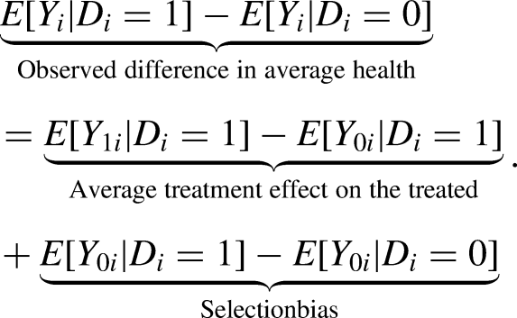
Now, consider a timeout as a treatment. The equivalent of an individual in our case is a team, and we consider teams in different years as different individuals.⁵ Simply comparing performance after a timeout with average performance in general would conflate the effect of the timeout with the deteriorating trend that prompted it. This is a textbook case of selection on unobservables that vary over time.

To overcome this issue, we follow two strategies. First, we exploit the panel structure of PbP data, and treat team-season combinations as individual observational units to consider direct measures of

E [Y_{1 i} | D_{i} = 1] - E [Y_{0 i} | D_{i} = 1] .

by constructing the difference in the performance of the same team in the minute before and the minute after the timeouts using different performance indicators and evaluating if their mean is statistically different from zero using non-parametric methods. Our primary within-team matching criterion is the performance difference immediately before and after the timeout (or non-timeout) event. In this team-based approach we control for additional standard observable factors including the game quarter, the number of substitutions during the run, and other conditions at the moment of the timeout call.

Second, we use a difference-in-differences (DiD) strategy. The idea is to compare the change in performance of teams following a timeout (treated group) with the change in performance of teams in similar situations where no timeout is called (control group). Specifically, we examine runs conceded by teams, comparing situations with and without a timeout. This method allows us to isolate the causal effect of the timeout from other confounding factors that might be influencing performance.

Formally, let $Y_{i t}$ denote the performance of team $i$ at time $t$ , and let $D_{i t} = 1$ if a timeout was called at time $t$ for team $i$ , and $D_{i t} = 0$ otherwise. The DiD estimator computes:

{\hat{δ}}_{D i D} = (E [Y_{i, t + 1} - Y_{i t} ∣ D_{i t} = 1]) - (E [Y_{i, t + 1} - Y_{i t} ∣ D_{i t} = 0]) .

This approach relies on the parallel trends assumption—that, in the absence of a timeout, the treated and control groups would have experienced similar changes in performance.

Equivalently, outcome trends are assumed to be the same for both groups in the counterfactual scenario without treatment. Formally, this condition can be expressed as the standard unconfoundedness assumption on potential outcomes:

E [Y_{0 i, t + 1} - Y_{0 i t} ∣ D_{i t} = 1] = E [Y_{0 i, t + 1} - Y_{0 i t} ∣ D_{i t} = 0]

which states that the pre-post change in performance for the treatment group would have followed the same trend as the pre-post change in the control group had the treatment group not been treated. As discussed and further assessed in Appendix B.1, we provide graphical evidence on pre-treatment dynamics to evaluate the plausibility of this assumption in our context. If the parallel trends assumption holds, the DiD estimate captures the true causal effect of the timeout, netting out time-varying confounders that affect both groups equally.

Possible violations of this assumption may arise if only one of the groups experiences a change in outcome trends for reasons unrelated to the treatment, or if there are differential changes in the composition of the treated and control groups. In the context of basketball games, such violations could occur if teams that call timeouts differ systematically from teams that do not in terms of coaching strategy, lineup quality, or other situational factors that independently affect subsequent performance. To increase the plausibility of the parallel trends assumption, we introduce a novel exercise that, to our knowledge, has not yet been explored. Specifically, we compute the difference-in-differences estimator comparing situations in which a team suffering a certain run calls a timeout with situations where the same team suffering a run has no timeouts left and is therefore unable to call one. This additional analysis further supports our main findings, as the results remain consistent even in this restricted setting. In this specific context, the parallel trends assumption is strengthened by the fact that both treated and control observations refer to the same team, coach, and roster, thereby addressing concerns about differential group composition. A potential concern with the comparison between timeout calls and situations in which no timeouts are left is that the latter may itself be endogenous to coaching strategy. We discuss further and show that our specification is robust to this possibility in Appendix B.2.

Moreover, our causal inference framework also relies on the Stable Unit Treatment Value Assumption (SUTVA). In this context, SUTVA requires that the effect of a timeout on a given run is not influenced by other nearby timeouts, either for the same team or the opponent. That is, each timeout constitutes a well-defined treatment whose effect is independent of the timing or occurrence of other timeouts. This assumption rules out interference across treatments and ensures that the potential outcomes associated with a given timeout are uniquely defined. We come back to the practical implementation of this assumption in Section “Direct Tests”. For these reasons, because the inability to call a timeout is mechanically determined by independent prior timeout usage rather than by contemporaneous confounders, this comparison reduces the scope for differential changes in outcome trends unrelated to the treatment. As a result, the treated and control situations differ only in the availability of a timeout, lending additional credibility to the causal interpretation of the DiD estimates.

Alternative approaches in the literature have relied on propensity score matching to address selection bias. For example, Assis et al. (2020), Gibbs et al. (2022), Weimer et al. (2023) apply propensity score matching on a range of observable factors, including team identities, betting lines, game time, run duration, estimated win probability, and player substitutions. These methods aim to balance observed covariates between treated and control groups drawn from different teams and game contexts.

However, we consider it very difficult to fully disentangle the effect of a game stoppage from coaches’ strategic changes and other team-level unobserved factors that could influence the outcome. Therefore, we match observations within the same team to account for team fixed effects, allowing us to keep constant the team’s characteristics and context, which is a standard application of the difference-in-differences approach and of the parallel trends assumptions. As a result, we interpret our estimate as reflecting the effect of the timeout in altering the course of the game.

The only remaining challenge is to define appropriate performance indicators. Building on the concept of runs and score differential impact we construct and analyze three indicators.

Off-Run Adjustment ( $ORA$ ): Captures how timeouts influence a team’s ability to stop sustained scoring droughts. It is defined as the difference in the average (across all games played by each team in the regular season) length of off-the-run streaks in the minute before and after a timeout.

On-Run Adjustment ( ${ORA}^{+}$ ): Measures how timeouts affect a team’s ability to sustain scoring momentum. It is the difference in the average (across all games played by each team in the regular season) length of on-the-run streaks in the minute before and after a timeout.

Score Differential Impact ( $SDI$ ): Quantifies the overall impact of timeouts on game score. It is computed as the difference between points scored by a team and points conceded in the minute preceding a timeout, compared to the minute following the timeout.

Game Box-Score data

We retrieve a rich set of game Box-Score variables through the API. This allows us to obtain a comprehensive list of elements, capturing the names of the teams and their respective coaches, individual player statistics (labeled PlayerStats) and aggregated team statistics (TeamStats) for all games.

Our use of Box-Score data

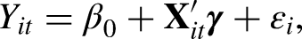
Since Play-by-Play data only allow for a local measure of the impact of timeouts—by evaluating team performance before and after a timeout–we complement this with an analysis of their global effect on performance. To do so, we use Box-Score data to estimate the standard four-factor model of wins, introduced by Oliver (2004) and described in Winston (2009) and Zuccolotto and Manisera (2020) and further developed in Migliorati et al. (2023) and Cecchin (2022). We then assess whether adding a fifth factor, capturing timeout efficiency, provides additional predictive power for wins beyond the standard four factors.

To define a season wide indicator of success timeouts we rely on the SDI. Formally, for team $a$ and timeout $t$ , the Score Differential Impact is defined as:

{SDI}_{a, t} = ({Points}_{a, t^{-}}^{made} - {Points}_{a, t^{-}}^{conceded}) - ({Points}_{a, t^{+}}^{made} - {Points}_{a, t^{+}}^{conceded}) .

where

t^{-}

denotes the one minute interval immediately preceding timeout

t

, and

t^{+}

denotes the one minute interval immediately following the timeout. Negative values of SDI indicate an improvement in performance after the timeout, while positive values suggest a deterioration. We define a timeout as successful if

{SDI}_{a, t} < 0

, indicating that the net point differential improves in the minute following the timeout relative to the minute preceding it. A season wide indicator of successful timeouts is then constructed for each team as the average number of successful time-outs per game over the course of the season.

In our baseline specification, we model performance using a one-minute window before and after each timeout. To ensure that our findings are not driven by the arbitrary choice of this window, we conduct a robustness analysis considering alternative time windows previously employed in the literature. For example, Gibbs et al. (2022) examine performance in the two minutes preceding a timeout and the one minute following it, while Weimer et al. (2023), within a different identification framework, evaluate performance over a three-minute interval after the timeout call. Across all these alternative specifications, our main results remain qualitatively and quantitatively unchanged, indicating that the estimated effects are not sensitive to the particular choice of the time window.⁶

Results using Play-by-Play data

We use PbP data to analyze the general features of time out calls. We analyze regular-season data from three seasons, excluding the final minute of each of the first three quarters and the final two minutes of the fourth quarter.⁷

Figure 1 reports the share of total timeouts called in the three seasons (4300) when the team was home or away, or on the run or off the run. The evidence shows that being home or away makes very little difference in determining the coach’s attitude toward timeouts, while being off the run is a crucial factor as over 95 per cent of timeouts are called when the team is off the run. Figure 2 offers a more granular perspective by reporting, for home and away games, the counts of timeouts as a function of opponents’ scoring runs, defined as consecutive points conceded to the opponent.

Figure 1.

When are timeouts called?

Figure 2.

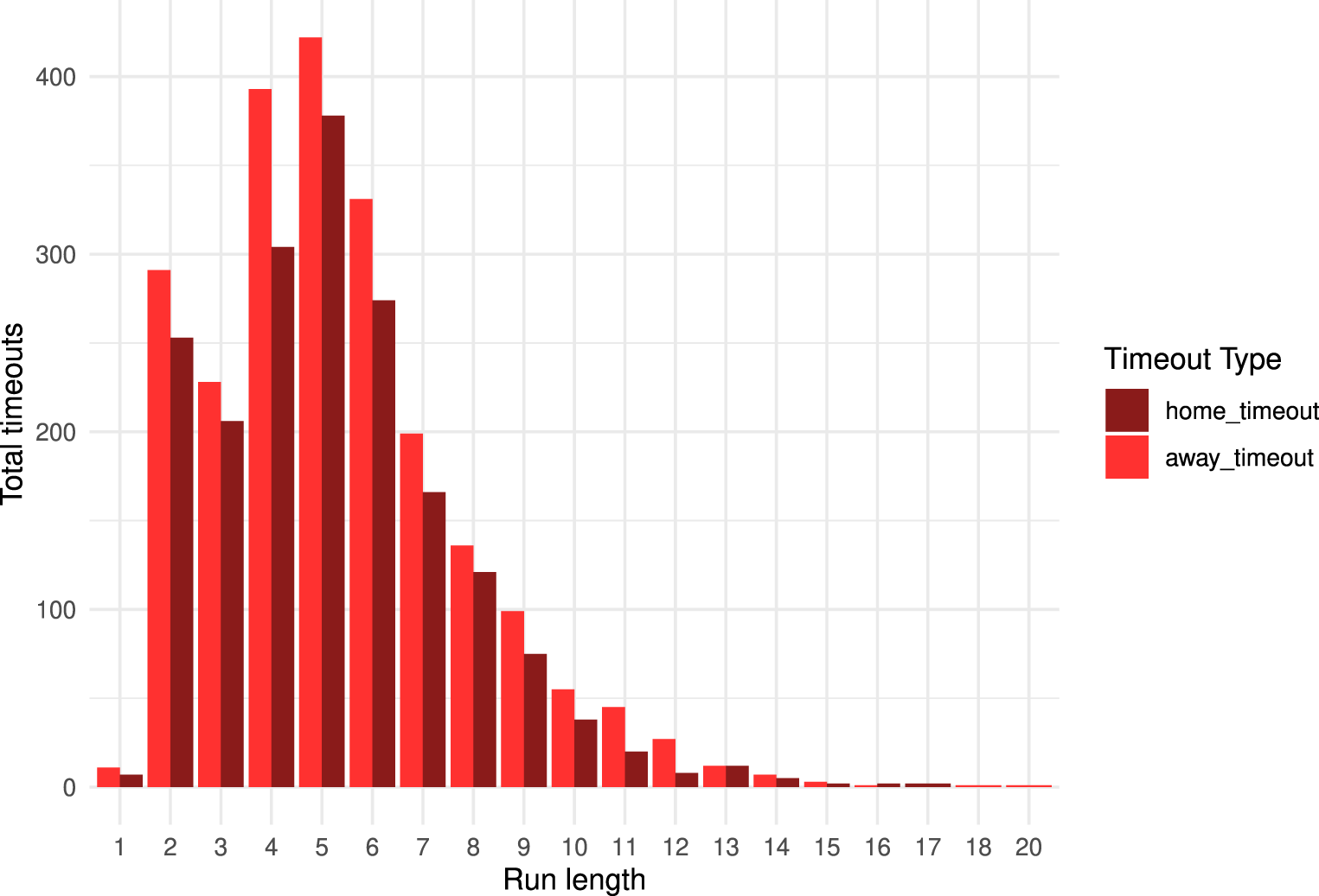
Home vs. Away Timeouts by opponents’ run.

The distribution exhibits a clear mode at five points, with the majority of timeouts occurring during runs of four to six points. Notably, a secondary local peak emerges at runs of two points, which may indicate a propensity among coaches to call a timeout immediately after their team relinquishes the lead. The distribution is homogenous for home and away games.⁸

Figures 3–5 present graphical evidence on the effects of timeouts on our three performance indicators, which are computed by taking the averages for each team in each season for a total of 54 observations (18 teams over 3 seasons). Each figure reports the individual observations for the indicator, together with the corresponding sample mean and a confidence interval defined as $\pm$ one standard deviation.

Figure 3.

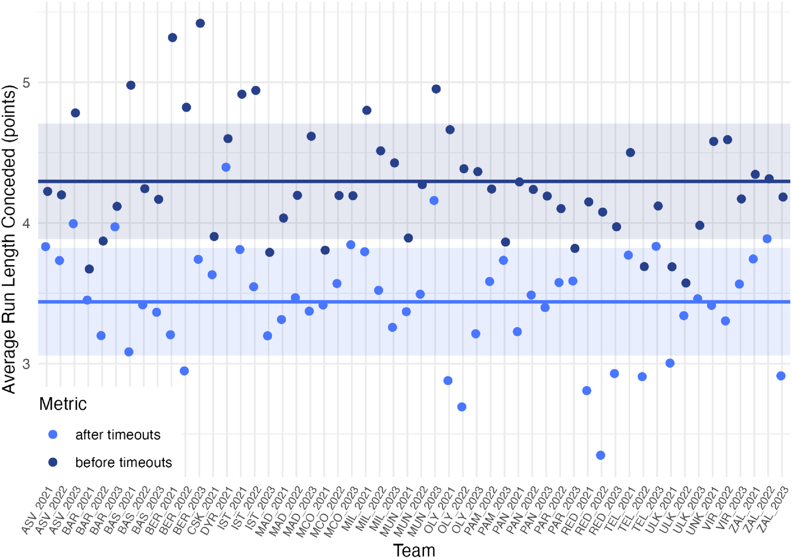
Average length of off-the-run streaks in the minute before and after a timeout.

Figure 4.

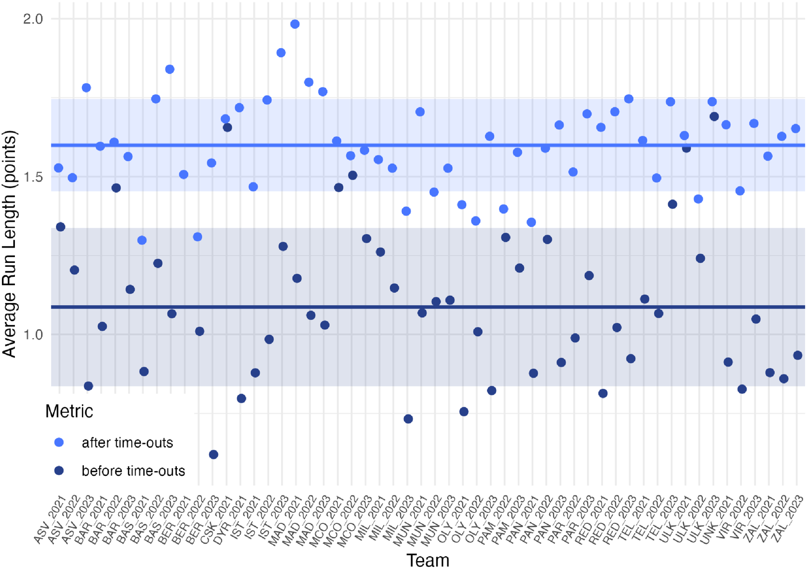
Average length of on-the-run streaks in the minute before and after a timeout.

Figure 5.

SDI: difference between points scored by a team and points conceded in the minute following a timeout, compared to the minute preceding the timeout.

Figures 3–4 indicate that timeouts exert some influence on the average lengths of both off-the-run and on-the-run streaks. While the figures provide a visual impression of timeout effectiveness as captured by these two indicators, the considerable width of the confidence intervals highlights the substantial uncertainty surrounding these estimates. The most informative evidence on the impact of timeouts on the score is provided by the Score Differential impact reported in Figure 5. The Figure shows that the difference between points scored by a team and points conceded is narrower in the minute following a timeout compared to the minute preceding it. However, the score differential never turns positive on average for any team, indicating that timeouts help limit losses but do not turn games around.

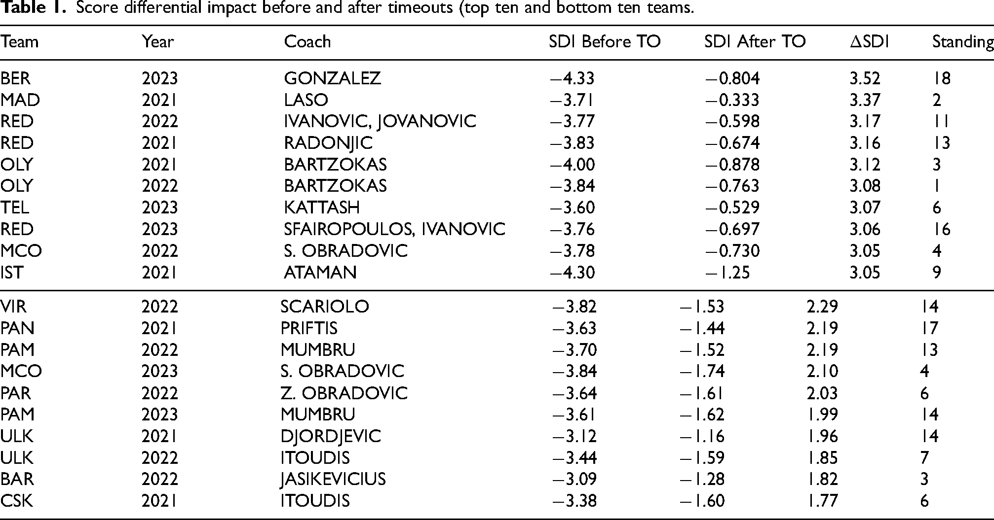
Table 1 complements the evidence by reporting the SDI for the top ten and the bottom ten teams in the league according to this criterion of timeout performance. Although SDI after timeouts are always smaller than SDI before timeouts, they never turn positive; not even for Israel Gonzalez, who is the most efficient coach in calling timeouts. It is also interesting to note that there is no clear pattern of association between timeouts effectiveness and standing of the team in the league at the end of the season. Again, Alba Berlin, the best performing team around timeouts, came last in the regular season 2022-23.

Table 1.

Score differential impact before and after timeouts (top ten and bottom ten teams.

Team	Year	Coach	SDI Before TO	SDI After TO	$Δ$ SDI	Standing
BER	2023	GONZALEZ	$-$ 4.33	$-$ 0.804	3.52	18
MAD	2021	LASO	$-$ 3.71	$-$ 0.333	3.37	2
RED	2022	IVANOVIC, JOVANOVIC	$-$ 3.77	$-$ 0.598	3.17	11
RED	2021	RADONJIC	$-$ 3.83	$-$ 0.674	3.16	13
OLY	2021	BARTZOKAS	$-$ 4.00	$-$ 0.878	3.12	3
OLY	2022	BARTZOKAS	$-$ 3.84	$-$ 0.763	3.08	1
TEL	2023	KATTASH	$-$ 3.60	$-$ 0.529	3.07	6
RED	2023	SFAIROPOULOS, IVANOVIC	$-$ 3.76	$-$ 0.697	3.06	16
MCO	2022	S. OBRADOVIC	$-$ 3.78	$-$ 0.730	3.05	4
IST	2021	ATAMAN	$-$ 4.30	$-$ 1.25	3.05	9

VIR	2022	SCARIOLO	$-$ 3.82	$-$ 1.53	2.29	14
PAN	2021	PRIFTIS	$-$ 3.63	$-$ 1.44	2.19	17
PAM	2022	MUMBRU	$-$ 3.70	$-$ 1.52	2.19	13
MCO	2023	S. OBRADOVIC	$-$ 3.84	$-$ 1.74	2.10	4
PAR	2022	Z. OBRADOVIC	$-$ 3.64	$-$ 1.61	2.03	6
PAM	2023	MUMBRU	$-$ 3.61	$-$ 1.62	1.99	14
ULK	2021	DJORDJEVIC	$-$ 3.12	$-$ 1.16	1.96	14
ULK	2022	ITOUDIS	$-$ 3.44	$-$ 1.59	1.85	7
BAR	2022	JASIKEVICIUS	$-$ 3.09	$-$ 1.28	1.82	3
CSK	2021	ITOUDIS	$-$ 3.38	$-$ 1.60	1.77	6

Direct tests

Our first strategy to gather statistical evidence on the causal effect of timeouts is to test directly the significance of the average treatment effect on the treated. In particular, we adopt the statistical tests used to measure performance differences in the same subjects under different conditions in medical research (pre/post treatment effects), finance (comparing investment returns), and psychology (effect of interventions) to the analysis of the differential team performance after the timeouts and before the timeouts. We implement two tests: the paired t-test, originally introduced by (Gosset, 1908),⁹ and the Wilcoxon text (Wilcoxon, 1945).¹⁰ As, as pointed out in Gibbs et al. (2022), a necessary assumption that must hold for our causal inference framework assumption is the Stable Unit Treatment Value Assumption (SUTVA): a timeout’s effect on a given run should not be influenced by other nearby timeouts. To limit potential interference, we retain only timeout observations that are isolated: specifically, we exclude any timeout for which another timeout occurs within a $\pm 120$ -second window, consistent with the practice in Gibbs et al. (2022). This filter isolates treatment events.

The paired $t$ -test (also known as the dependent $t$ -test) is a parametric statistical test used to compare the means of two related groups. It assesses whether there is a significant difference between the means of two dependent samples, typically taken from the same individuals before and after an intervention, in our case the performance of the same team before and after the timeout. The paired $t$ -test is based on the difference between paired observations, which are assumed to be normally distributed:

d_{i} = X_{i, 1} - X_{i, 2}

where

d_{i}

is the difference between the paired values. The test statistic is calculated as:

t = \frac{\bar{d}}{s_{d} / \sqrt{n}}

where:

\bar{d}

= mean of the differences,

s_{d}

= standard deviation of the differences,

n

= number of paired observations. The test follows a

t

-distribution with

n - 1

degrees of freedom. The null hypothesis is that of no difference between means, our alternative hypothesis of interest is that the mean difference has a specific direction in the sense that timeouts have a positive impact on teams’ performances and we therefore consider a one-tailed alternative. The Wilcoxon signed-rank test is a non-parametric statistical test used to the same end with the paired t-tests, it is considered as a viable alternative robust to the violation of the assumption of normality. The key assumptions are still paired observations or continuous or at least ordinal data but the assumptions of normality is substituted with that of symmetry : the distribution of the differences between paired data should be approximately symmetric around the median. Given a set of paired observations

(X_{i, 1}, X_{i, 2})

, the test is constructed by computing the differences:

d_{i} = X_{i, 1} - X_{i, 2}

Ignoring zeros, the absolute differences

| d_{i} |

are ranked from smallest to largest. The test statistic is given by:

W = \sum R_{+}

where

R_{+}

is the sum of ranks corresponding to positive differences. The distribution of

W

under the null hypothesis can be approximated using the normal distribution for large sample sizes. The null hypothesis is that the median difference between paired observations is zero, the alternative hypothesis is again one-tailed.

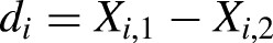
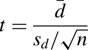
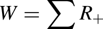
Table 2 reports the results of the implementation of the two tests to (i) the difference between paired Average length of off-the-run streaks in the minute before and after a timeout (ORA), (ii) the difference between paired Average length of on-the-run streaks in the minute before and after a timeout ( ${O R A}^{+}$ ), and (iii) the difference between points scored and conceded in the minute before paired with the difference between points scored and conceded in the minute following a timeout (SDI).

Table 2.

One-sided paired tests for (i) the difference between paired average length of off-the-run streaks in the minute before and after a timeout (ORA), (ii) the difference between paired average length of on-the-run streaks in the minute before and after a timeout ( ${O R A}^{+}$ ), and (iii) the difference between points scored and conceded in the minute before paired with the difference between points scored and conceded in the minute following a timeout (SDI).

	ORA	$O R A^{+}$	SDI
Paired t-test	${\frac{1.09}{0.062}}^{* * *}$	${\frac{- 0.61}{0.034}}^{* * *}$	${\frac{- 2.54}{0.06}}^{* * *}$
Wilcoxon test	54 $^{* * *}$	0 $^{* * *}$	0 $^{* * *}$

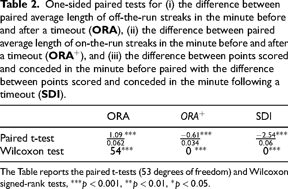
The Table reports the paired t-tests (53 degrees of freedom) and Wilcoxon signed-rank tests, $^{* * *} p < 0.001$ , $^{* *} p < 0.01$ , $^{*} p < 0.05$ .

The statistical results indicate that the null hypothesis is consistently rejected, implying that timeouts have a statistically significant effect in limiting losses. To assess the magnitude of this effect, consider the case of the SDI. The estimated average difference between points scored and points conceded in the minute before the timeout and the minute after is –2.54. This implies that timeouts locally improve team performance by 2.54 points on average, and the null hypothesis that this effect equals zero is rejected at the 1 per cent significance level. However, timeouts do not reverse the overall scoring imbalance. Teams calling a timeout continue to concede more points than they score: although the point differential in the minute after the timeout is less negative than in the minute before, it remains positive, indicating that timeouts mitigate losses but do not fully eliminate them.

This evidence is robust to a series of robustness checks designed to assess the stability of our results. Across all specifications the sign and magnitude of the estimated effects—and their statistical significance—remain in line with our main findings.

Our robustness analysis is well illustrated by a model representation of our approach for the SDI index of performance. We consider a linear model for the conditional expectation of SDI that incorporates both the timeout indicator and a vector of relevant covariates. Let $Y_{i t}$ denote the SDI measured around a timeout taken at time $t$ for team $i$ . Let $X_{i t}$ denote a vector of control variables capturing contextual factors such as team fixed effects, opponent fixed effects, quarter or time-within-game indicators, score difference before the timeout, and any other relevant characteristics. The model we estimate is:

E [Y_{i t} ∣ X_{i t}] = β_{0} + X_{i t}^{'} γ,

which leads to the empirical specification

Y_{i t} = β_{0} + X_{i t}^{'} γ + ε_{i},

where

ε_{i}

is the error term.

The coefficient of interest is $β_{0}$ , which measures the expected SDI in the minute before and the minute after a timeout, conditional on the covariates in $X_{i t}$ . A negative value of $β_{0}$ indicates an improvement in scoring performance after a timeout relative to comparable situations without a timeout. The inclusion of covariates allows us to account for differences in team strength, game context, and strategic conditions, making the estimation more robust to potential confounding factors. Specifically we define the following covariates:

$X_{1, i t}$ : dummy for the final quarter of the game

$X_{2, i t}$ : dummy for runs before the timeout higher then six points (Weimer et al., 2023)

$X_{3, i t}$ : dummy to exclude final three minutes when either team leads by at least 20 points, (Weimer et al., 2023)

$X_{4, i t}$ : dummy for lineup changes during the timeout

The results from the estimation of the linear model are reported in Table 3. The model is estimated on all data points (without averaging across teams and seasons), for a total of 2879 observations.

Table 3.

Linear models for SDI.

	Model 1	Model 2
Intercept	$- {2.528}^{* * *}$	$- {1.797}^{* * *}$
	$(0.053)$	$(0.099)$
$X_{1, i t}$		$- 0.048$
		$(0.120)$
$X_{2, i t}$		$- {1.493}^{* * *}$
		$(0.103)$
$X_{3, i t}$		$- 0.047$
		$(0.106)$
$X_{4, i t}$		$- 0.670$
		$(0.418)$
Residual std. error	2.846 (df $=$ 2878)	2.748 (df $=$ 2874)
$R^{2}$	–	0.0688
Adjusted $R^{2}$	–	0.0675
F-statistic	–	53.1 ( $p < 0.001$ )

Notes: Standard errors in parentheses. $^{* * *} p < 0.001$ , $^{* *} p < 0.01$ , $^{*} p < 0.05$ .

The intercept of the model can be interpreted as the expected value of the Scoring Differential Index (SDI) and it matches the $- 2.54$ in Table 2. The inclusion of covariates as controls reduces the point estimate of this coefficient to $- 1.8$ but the lowest point of the 95 per cent confidence interval is still well above zero at $- 1.6$ . The only significant control is $X_{2, i t}$ , the dummy for runs before the timeout higher then six points. The effect of timeouts called to stop runs higher than six points is estimated at a reduction of the scoring differential of 3.3 points, which is significantly larger than the baseline effect of 2.54 points. Overall, the regression results indicate that successful defensive timeouts have a positive and statistically significant effect on short-run scoring performance, even after accounting for game context and team-specific factors. However, although timeouts improve SDI, the improvement is not large enough on average to reverse the scoring deficit entirely: the post-timeout SDI remains negative, albeit less negative than before. To reconcile graphical and econometric evidence Figure 1 shows that the difference between points scored and points conceded averages $- 3.74$ before a timeout and $- 1.2$ after a timeout. Although the timeout significantly reduces this gap by 2.54 points, the difference remains negative. Moreover, to assess whether these results are driven by persistent differences across teams, we perform a robustness analysis allowing for team fixed effects. As discussed in Appendix C, we find no statistically significant evidence of team-level heterogeneity in the scoring differential around timeouts, supporting the pooled interpretation of the baseline estimates.

The evidence from Diff-in-Diff test

Our second empirical strategy is based on a setting that approximates a quasi–natural experiment: we compare runs conceded by a team to runs conceded when no timeouts are left, i.e., when the coach cannot halt momentum to reorganize the team or implement strategic adjustments. This comparison provides a plausibly exogenous counterfactual for the effect of calling a timeout. As shown in Figure 6 and Table 4, the results align with our main finding, both graphically and statistically. Figure 6 show that timeouts have some impact on the average length of off-the run streaks, where off-the run streaks are considerable higher when the coach does not have the possibility to call a timeout with respect to the case where timeouts are available.

Figure 6.

Difference between off-the run streaks conceded by a team and off-the run streaks conceded when no timeouts are left for the coach.

Table 4.

One-sided paired tests for the difference between paired averages: avg run conceded before vs. after (no timeout to the left).

	Avg run conceded
Paired t-test	${\frac{- 0.54}{0.071}}^{* * *}$
Wilcoxon test	100 $^{* * *}$

The table reports the paired t-test (53 degrees of freedom) and Wilcoxon signed-rank test; $^{* * *} p < 0.001$ , $^{* *} p < 0.01$ , $^{*} p < 0.05$ .

Table 4 reports the results of the implementation of the two tests of the previous section to the difference between paired Average length of off-the-run streaks conceded by a team during the whole game vs off-the-run streaks conceded when no timeouts are left.

Both tests point in the same direction: the paired mean difference is negative ( $\bar{d} = - 0.51$ ), and the paired $t$ -test is highly significant ( $t = - 7.27$ ). The Wilcoxon signed-rank test likewise rejects, indicating that the result does not hinge on normality assumptions or sensitivity to outliers. Overall, the average run conceded by a team is systematically lower than its counterpart when no timeout are left, confirming the robustness of the main findings.

Limitations

Although our results are robust across multiple empirical approaches, they should be interpreted in light of their limitations. First, our analysis focuses on short-run outcomes measured in narrowly defined post-timeout windows, which limits the potential impact of confounding factors but may not fully capture longer-lasting tactical or psychological effects that unfold over extended stretches of the game. Second, although we control for a rich set of contextual variables, in the case of relevant omitted variables, even combined non-parametric and parametric approaches may not fully isolate causal effects. A related limitation concerns the potential endogeneity of timeout usage to gameplay dynamics. In particular, timeouts may not be entirely exogenous to performance changes, especially during the regular season. Early in the season, coaches may use timeouts to experiment with specific plays, lineups, or tactical adjustments, rather than solely to interrupt opponent momentum. As a result, the state of being without timeouts left—while central to our identification strategy—may itself reflect earlier strategic experimentation or learning processes that evolve over the course of the season. Future research could address this concern by focusing on playoff games or late-season matchups, where coaching strategies and team mechanisms are more stable, thereby reducing the scope for experimentation-driven timeout usage and strengthening the exogeneity of timeout availability. Early in the season, timeout usage may reflect coaching experimentation with plays, lineups, or tactical adjustments rather than efforts to interrupt opponent momentum. Consequently, the absence of remaining timeouts, while central to our identification strategy, could partly capture earlier strategic choices or learning processes that vary over the course of the season. We address this concern by explicitly examining later-season matchups, as detailed in Appendix B.2, where incentives are clearer and strategic behavior is more stable. Nonetheless, further strengthening the exogeneity of timeout availability remains an important avenue for future research. In particular, focusing on playoff games or on high-stakes regular-season matchups, such as contests involving teams at the top of the standings or well established rivalries, could further limit the role of experimentation in timeout usage and provide an even cleaner setting for causal identification.

Third, our analysis relies exclusively on regular-season Euroleague data, which complements the evidence for the NBA but may limit the generalization of the findings to other less important leagues or stages of the competition.

Results using Box-Score data

The evidence from Play-by-Play data suggests that timeouts have a statistically significant, yet modest, local effect. This finding naturally raises the question of their impact on overall team performance. Although timeouts appear to mitigate losses during critical phases of the game, they do not necessarily alter its eventual course. The relevant issue, then, is whether one can identify any systematic influence of timeouts on team performance over the regular season, as measured by Box-Score data.

To address this question, we specify first a standard model that links basketball performance measured by wins in a regular season¹¹ to a few key factors, to then investigate whether a factor measuring timeout efficiency adds explanatory power.

Our benchmark model is the Oliver’s four-factor model of wins (Oliver, 2004, which models teams’ wins in the regular season as a linear function of four indicators. These indicators are used to parsimoniously aggregate team statistics across different performance dimensions. The dimensions considered are Shooting, Turnovers, Rebounding, and Free Throws and Fouls.

The four factors are constructed for each team $i$ entering the EuroLeague in season $t$ as follows:

$F 1_{i, t} = E F G_{i, t} - O E F G_{i, t}$

– EFG = $\frac{Field\ Goals\ Made + 0.5 \times 3 - Point\ Field\ Goals\ Made}{Field\ Goal\ Attempts}$

– OEFG = $\frac{Field\ Goals\ Made\ by\ Opponents + 0.5 \times 3 - P o i n t F i e l d G o a l s M a d e b y O p p o n e n t s}{Field\ Goal\ Attempts\ by\ Opponents}$

$F 2_{i, t} = T P P_{i, t} - O T P P_{i, t}$

– TPP = $\frac{Turnovers}{Employed\ Possessions}$

– OTPP = $\frac{Opponent\ Turnovers}{Acquired\ Possessions}$

– Employed Possession = $Field\ Goal\ Attempts + 0.45 \times Free\ Throws + Turnovers - Offensive\ Rebounds$

–Acquired Possession = Opponent Turnovers + Defensive Rebounds + Team Rebounds + Opponent Field Goal Attempts + 0.45 × Opponent Free Throws

$F 3_{i, t} = O R P_{i, t} + D R P_{i, t}$

– ORP = $\frac{Offensive\ Rebounds}{Total\ Missed\ Shots}$

– DRP = $1 - \frac{Opponent\ Offensive\ Rebounds}{Total\ Opponent\ Missed\ Shots}$

$F 4_{i, t} = F T R_{i, t} - O F T R_{i, t}$

– FTR = $\frac{Foul\ Shots\ Made}{Field\ Goal\ Attempts}$

– OFTR = $\frac{Opponent\ Foul\ Shots\ Made}{Opponent\ Field\ Goal\ Attempts}$

The first factor captures the relative shooting efficiency, measured via the Effective Field Goal Percentage (EFG), compared to the Opponents’ Field Goal Percentage (OEFG). EFG is calculated by appropriately weighting two-point and three-point shots made.

The second factor measures the relative efficiency of teams and their opponents in utilizing possessions, using Turnover Per Possession (TPP) as the efficiency indicator. Employed and Acquired Possessions are nearly equal by construction. A possession refers to the period during which one team controls the ball and attempts to score. It starts when a team gains the ball and ends when the team either scores or turns it over. A possession may also include multiple plays, and offensive rebounds can extend the same possession. Free throws are weighted at 0.45 in the definition of possession due to the occurrence of ”and-one” situations.

The third factor accounts for the relative rebounding abilities by combining Offensive Rebound Percentage (ORP) and Defensive Rebound Percentage (DRP).

Finally, the fourth factor focuses on free throws and fouls, using the Free Throw Ratio (FTR), which is the ratio of Foul Shots Made to Field Goal Attempts. This factor captures both the effectiveness of drawing fouls on shooters and capitalizing on free throws.

To assess the explanatory power of the four factors in accounting for team performance, we begin with the standard approach and estimate the following regression using pooled cross-sectional data from all available seasons.¹² However, we later relax the pooling assumption as part of our robustness analysis.

The following model, where the total number of wins for each team in each season $W_{i t}$ is linearly related to the four factors, is estimated:

\begin{aligned} W_{i t} & = β_{0} + γ_{0} D_{t}^{2021 - 2022} + γ_{1} D_{t}^{R U S} + β_{1} F 1_{i t} + β_{2} F 2_{i t} \\ + β_{3} (F 3_{i t} - 1) + β_{4} F 4_{i t} + ϵ_{i t} v_{i t} \sim N . I . D (0, σ^{2}) \end{aligned}

(1)

Note that in the 2021–2022 EuroLeague season, the expulsion of the Russian teams (CSKA Moscow, Zenit Saint Petersburg, and UNICS Kazan) resulted in a reduced number of regular-season games. The reduction in the number of games was different for the Russian teams and the other teams. Therefore, we introduce two dummies in our specification: $D_{t}^{2021 - 2022}$ , which takes a value of 1 for all teams in the 2021-2022 season and 0 otherwise, and $D_{t}^{R U S}$ , which takes a value of 1 for Russian teams in the 2021-2022 season and 0 otherwise.

The model has a very natural interpretation: all factors take the value of zero for the average team in the league, because the average team in the league performs exactly as the average opponent.¹³ The constant in the regression captures the number of wins in the season of the average team, which is half of the game played, while the coefficients on each of the factors capture the contribution of each factor to explain, for each team and each season, higher number of wins with respect to the marginal team. The expected sign of the coefficients on the factors are positive for $F 1_{i t}, (F 3_{i t} - 1)$ , and $F 4_{i t}$ , in that Scoring Efficiency, Rebounding and Free-Throw efficiency contribute positively to performance, while it is negative for $F 2_{i t}$ , in that turnovers contribute negatively to performance. Having established a baseline model of performance, we extend it to assess the potential impact of timeout efficiency by adding a fifth factor that captures how effectively a team uses its timeouts:

$F 5_{i, t} = S D I A_{i, t}$

– SDIA = the average number of successful timeouts per game SDI for team i in season t

We then estimate the following augmented model: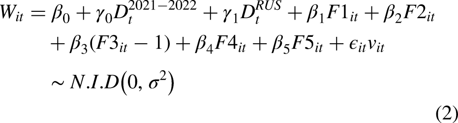

\begin{aligned} W_{i t} & = β_{0} + γ_{0} D_{t}^{2021 - 2022} + γ_{1} D_{t}^{R U S} + β_{1} F 1_{i t} + β_{2} F 2_{i t} \\ + β_{3} (F 3_{i t} - 1) + β_{4} F 4_{i t} + β_{5} F 5_{i t} + ϵ_{i t} v_{i t} \\ \sim N . I . D (0, σ^{2}) \end{aligned}

(2)

In this specification the significance of the coefficient on $F 5_{i t}$ , which is included as demeaned, captures the incremental contribution of timeouts efficiency as a factor for performance. The results from the estimation of the two models are reported in Table 5.

Table 5.

The four-factor model and the five-factor model with a timeout efficiency factor.

	Dependent variable: $W_{i t}$
	Four-Factor Model	Five-Factor Model
Intercept	16.95 $^{* * *}$	16.97 $^{* * *}$
	(0.33)	(0.32)
$D_{t}^{2021 - 2022}$	−0.94	−0.96
	(0.60)	(0.60)
$D_{t}^{R U S}$	−2.83 $^{*}$	−2.98 $^{*}$
	(1.27)	(1.26)
${F 1}_{i t}$	105.02 $^{* * *}$	103.50 $^{* * *}$
	(9.06)	(9.03)
${F 2}_{i t}$	−101.49 $^{* * *}$	−100.51 $^{* * *}$
	(14.54)	(14.40)
${F 3}_{i t} - 1$	50.26 $^{* * *}$	52.28 $^{* * *}$
	(8.34)	(8.37)
${F 4}_{i t}$	15.32 $^{*}$	17.07 $^{* *}$
	(5.74)	(5.81)
${F 5}_{i t}$		−0.99
		(0.69)
Observations	54	54
Residual Std. Error	1.94 (df $=$ 47)	1.96 (df $=$ 46)
Multiple R²	0.86	0.86
Adjusted R²	0.84	0.84
F Statistic	47.25 (6, 47)	41.68 (7, 46)

$^{* * *} p < 0.001$ , $^{* *} p < 0.01$ , $^{*} p < 0.05$ .

The estimation of the four-factor models reveals that all coefficients are statistically significant with positive values for the coefficients on $F 1_{i t}, (F 3_{i t} - 1)$ , and $F 4_{i t}$ , and a negative value for the coefficient on $F 2_{i t}$ . The factors explain 0.84% of the variance of Wins. When the five-factor model is estimated, the null that the coefficient on the timeout factors is not statistically different from zero cannot be rejected, the estimates for all other coefficients are virtually unchanged, and the $R^{2}$ for the five-factor model is equal to that of the four-factor model. Therefore, the semi-partial $R^{2}$ associated with the timeout factor, capturing its marginal contribution to the overall explanatory power of the regression, is zero. Figure 7 illustrates graphically the point showing the absence of a relationship between the residuals from the four-factor model regression and factor $F 5_{i t}$ .

Figure 7.

The 5-th factor (timeouts) and the residuals from the standard 4-factor model for Wins.

Despite the intuitive structure and interpretability of the pooled cross-sectional specification, by stacking team–year observations and treating them as independent, the model implicitly assumes the absence of unobserved team-specific heterogeneity, independence across repeated observations for the same team, and stability of the relationships between performance factors and wins across seasons. For this reason, we additionally estimate a fixed-effects model that includes both team fixed effects (capturing all time-invariant unobserved characteristics) and year fixed effects (capturing league-wide shocks, rule changes, or seasonal disruptions such as the 2021–2022 Russian team expulsions). This panel-data specification relaxes the strong independence assumptions of the pooled model and allows the estimated coefficients to be interpreted as within-team effects over time. We also report standard errors clustered at the team level. The fixed-effects estimates serve as a robustness check and provide a more credible assessment of the marginal contribution of the four traditional factors and the proposed timeout efficiency factor to team performance. The model specification becomes the following: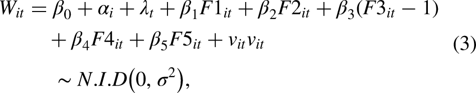

\begin{aligned} W_{i t} & = β_{0} + α_{i} + λ_{t} + β_{1} F 1_{i t} + β_{2} F 2_{i t} + β_{3} (F 3_{i t} - 1) \\ + β_{4} F 4_{i t} + β_{5} F 5_{i t} + v_{i t} v_{i t} \\ \sim N . I . D (0, σ^{2}), \end{aligned}

(3)

The results from the estimation of the 4 and 5 factors models are reported in Table 6.

Table 6.

Five-factor model with team and year fixed effects.

	Dependent variable: $W_{i t}$
	Five-Factors Model (Team + Year FE)
${F 1}_{i t}$	114.08 $^{* * *}$
	(14.41)
${F 2}_{i t}$	−128.60 $^{* * *}$
	(27.46)
${F 3}_{i t} - 1$	48.79 $^{* *}$
	(15.55)
${F 4}_{i t}$	20.49 $^{*}$
	(7.44)
${F 5}_{i t}$	−0.79
	(0.57)
Observations	51
Sum of Squared Residuals (SSR)	99.49
RMSE	1.40
Within R²	0.71

Team and year fixed effects included. Clustered SEs at team level.

$^{* * *} p < 0.001$ , $^{* *} p < 0.01$ , $^{*} p < 0.05$ .

The fixed-effects regression delivers results that are remarkably similar to those obtained from expanding the standard four factor model (Oliver, 2004). The signs, magnitudes, and statistical significance of the first four coefficients remain essentially unchanged, and the estimated coefficient on the timeout efficiency factor continues to be statistically indistinguishable from zero. This robustness to the inclusion of team and year fixed effects confirms that the earlier findings are not driven by omitted, time-invariant structural characteristics of teams or by season-level common shocks.

Conclusion

This paper evaluated Euroleague coaches’ timeout strategies, focusing on their local impact during games and their broader effect on team performance over a season. Using Play-by-Play data, our main findings are that timeouts help reduce scoring deficits, but they do not, on average, reverse the score differential in favor of the calling team. In other words, timeouts mitigate losses but do not turn games around. To assess whether timeouts contribute to long-term team success, we extend the standard Four-Factor Model of Wins for the analysis of the drivers of teams’ performances over the course of regular seasons by incorporating an SDI-based factor. The results show that the four standard factors have a strong explanatory power for team performance, and the timeout factor provides no additional predictive power. So, do timeouts matter in the Euroleague? Yes, but only in a limited sense. Timeouts are moderately useful for slowing opponents’ momentum, but they do not significantly alter game outcomes or contribute to long-term team success. The practical implications for coaches of our evidence are that substitutions during a timeout do not contribute to increase their local impact on the game and that the local effect of a timeout is higher if it is called after a scoring run of the opponent team of at least six points.

This study provides a foundation for several extensions in future work. First, future research may focus on the external validity of our evidence by assessing whether timeouts may matter more in different contexts. In particular, playoff games, with their higher stakes, tighter rotations, and slower pace, may offer a setting where timeouts have a stronger or more strategic impact than in the regular season. Moreover, focusing on playoff games or on high-stakes regular-season matchups, such as games involving teams at the top of the standings or well established rivalries, could further limit the role of experimentation in timeout usage and provide an even cleaner setting for causal identification. Second, is to explore alternative statistical models, such as in-game win probability models, state-dependent scoring models and regression discontinuity approaches, that may capture more complex ways in which timeouts influence performance. Third, and more importantly from an identification perspective, future research could go beyond estimating the reduced-form effect of a timeout being called and aim to disentangle the effect of the timeout itself from coaches’ strategic adjustments that occur during the timeout. Timeouts simultaneously interrupt momentum and provide an opportunity for tactical changes, such as calling specific offensive schemes or altering defensive strategies (switching from man-to-man to zone defense). Isolating these channels would require more granular Play-by-Play and tactical data. Leveraging such information would allow researchers to separately identify momentum-stopping effects from strategic coaching decisions, thereby providing a deeper understanding of the mechanisms through which timeouts affect game outcomes.

Footnotes

ORCID iDs

G Carta

CA Favero

Funding

The author(s) received no financial support for the research, authorship, and/or publication of this article.

Declaration of conflicting interests

The author(s) declared no potential conflicts of interest with respect to the research, authorship, and publication of this article.

Notes

Appendix

References

Allgrunn

Douglas

Wai

(2024) Optimal timeout choices in clutch situations in the nba. Journal of Sports Economics 25(2): 217–230.

Angrist

Pischke

(2009) Mostly Harmless Econometrics: An Empiricist’s Companion. Princeton NJ: Princeton University Press.

Assis

Assunção

Vaz-de Melo

(2020) Stop the clock: Are timeout effects real? In: Joint European conference on machine learning and knowledge discovery in databases, pp.507–523. Springer.

Berri

Schmidt

Brook

(2006) The Wages of Wins: Taking Measure of the Many Myths in Modern Sport. Stanford CA: Stanford University Press.

Cecchin

(2022) Oliver’s four-factor model: Validation through causality. International Journal of Sports Science & Coaching 17(4): 838–847.

Eurohoops (2021) Can a time-out stop a negative run? https://www.eurohoops.net/en/trademarks/1277233/euroleague-can-a-time-out-stop-a-negative-run/. Online article.

Galiani

Gertler

Schargrodsky

(2005) Water for life: The impact of the privatization of water services on child mortality. Journal of Political Economy 113(1): 83–120.

Gibbons

Chakraborti

(2010) Nonparametric Statistical Inference. 5th edition. Boca Raton, FL: CRC Press.

Gibbs

Elmore

Fosdick

(2022) The causal effect of a timeout at stopping an opposing run in the NBA. The Annals of Applied Statistics 16(3): 1359–1379.

10.

Gosset

(1908) The probable error of a mean. Biometrika 6(1): 1–25.

11.

Hogg

Tanis

Zimmerman

(2015) Probability and Statistical Inference. 9th edition. Harlow England: Pearson.

12.

Hollander

Wolfe

Chicken

(1999) Nonparametric Statistical Methods. 2nd edition. Hoboken, NJ: John Wiley & Sons.

13.

Iatropoulos

Sarlis

Tjortjis

(2025) A data mining approach to identify NBA player quarter-by-quarter performance patterns. Big Data and Cognitive Computing 9(4): 74.

14.

Migliorati

Manisera

Zuccolotto

(2023) Integration of model-based recursive partitioning with bias reduction estimation: A case study assessing the impact of Oliver’s four factors on the probability of winning a basketball game. AStA Advances in Statistical Analysis 107(1): 271–293.

15.

Oliver

(2004) Basketball on Paper: Rules and Tools for Performance Analysis. Washington, D.C.: Potomac Books, Inc.

16.

Permutt

(2011) The efficacy of momentum-stopping timeouts on short-term performance in the National Basketball Association. PhD Thesis.

17.

Vázquez-Estévez

Prieto-Lage

Silva-Pinto

, et al. (2025) Analysis of offensive patterns after timeouts in critical moments in the euroLeague 2022/23. Applied Sciences 15(3): 1580.

18.

Vergara

(2025) Analyzing NBA timeouts. https://medium.com/@ivm9816/analyzing-nba-timeouts-29df987f076a. Medium blog post.

19.

Weimer

Steinert-Threlkeld

Coltin

(2023) A causal approach for detecting team-level momentum in NBA games. Journal of Sports Analytics 9(2): 117–132.

20.

Wilcoxon

(1945) Individual comparisons by ranking methods. Biometrics Bulletin 1(6): 80–83.

21.

Winston

(2009) Mathletics. Princeton university press.

22.

Zuccolotto

Manisera

(2020) Basketball Data Science: with Applications in R. Boca Raton, FL: CRC Press.

Do timeouts matter? A study of euroleague Basketball *

Abstract

Keywords

Introduction

Placing our contribution in the literature

Methodology

Play-by-Play data

Our use of Play-by-Play data

Game Box-Score data

Our use of Box-Score data

Results using Play-by-Play data

Direct tests

The evidence from Diff-in-Diff test

Limitations

Results using Box-Score data

Conclusion

Footnotes

ORCID iDs

Funding

Declaration of conflicting interests

Notes

Appendix

References