Sage Journals: Discover world-class research

Abstract

This system allows the high-throughput protein interaction analysis on microarrays. We apply the interference technology 1λ–imaging reflectometric interferometry (iRIf) as a label-free detection method and create microfluidic flow cells in microscope slide format for low reagent consumption and lab work compatibility. By now, most prominent for imaging label-free interaction analyses on microarrays are imaging surface plasmon resonance (SPR) methods, quartz crystal microbalance, or biolayer interferometry. SPR is sensitive against temperature drifts and suffers from plasmon crosstalk, and all systems lack array size (maximum 96 spots). Our detection system is robust against temperature drifts. Microarrays are analyzed with a spatial resolution of 7 µm and time resolution of ≤50 fps. System sensitivity is competitive, with random noise of <5 × 10⁻⁵ and baseline drift of <3 × 10⁻⁶. Currently available spotting technologies limit array sizes to ~4 spots/mm² (1080 spots/array); our detection system would allow ~40 spots/mm² (10,800 spots/array). The microfluidic flow cells consist of structured PDMS inlays sealed by versatilely coated glass slides immobilizing the microarray. The injection protocol determines reagent volumes, priming rates, and flow cell temperatures for up to 44 reagents; volumes of ≤300 µL are validated. The system is validated physically by the biotinylated bovine serum albumin streptavidin assay and biochemically by thrombin aptamer interaction analysis, resulting in a KD of ~100 nM.

Keywords

high-throughput protein analysis imaging label-free detection reflectometric interferometry microfluidic biosensor

Introduction

Label-free technologies for the analysis of molecule-molecule interactions have the intrinsic advantage of no requirement for an additional label (e.g., an isotope, a fluorescent dye, a fluorescent protein, an enzyme, or a nanoparticle). These labels could at least make the system more artificial¹ and change the binding behavior of the system. Several label-free detection methods, e.g. high-performance liquid chromatography–mass spectrometry (HPLC-MS), nuclear magnetic resonance (NMR), calorimetry, allow the determination of affinity. Especially biosensor based methods, e.g. surface plasmon resonance (SPR)2, quartz crystal microbalance (QCM)3, biolayer interferometry (BLI)4, and reflectometric interference spectroscopy (RIfS)1, determine affinity and provide detailed insights into molecular kinetics on single spots or even microarrays. However, biosensors implicate one reactant to be immobilized while maintaining its initial activity.

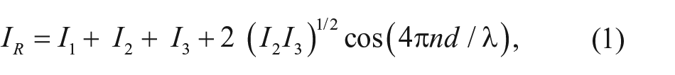
While SPR systems measure changes in the refractive index via SPR,⁵ relying on the evanescent field of electromagnetic radiation, RIfS detects changes in the optical thickness of the reagent binding layer (product of physical thickness and refractive index)⁶ and measures changes in the amplitude and phase of reflected polarized beams. Reflection is caused by multiple thin-layer interfaces: physical or (bio)chemical. If the coherence length of these reflected beams is longer than the optical path through the layers, they interfere and form an interference pattern depending on the optical thickness of the layers, the incident angle, and the refractive index of the surrounding medium.⁷ In the case of perpendicular incidence, a nonabsorbing layer, and low reflectance I₀ ( Fig. 1B ), the reflectance I_R is given by

I_{R} = I_{1} + I_{2} + I_{3} + 2 {(I_{2} I_{3})}^{1 / 2} \cos (4 π n d / λ),

Figure 1.

(A) 1λ–imaging reflectometric interferometry (iRIf) evolved from reflectometric interference spectroscopy (RIfS) measures the intensity change due to molecule adsorption at a specific wavelength. (B) Thin film stack, with a glass slide thickness of 1 mm and a refractive index of 1.52, is coated with semireflective thin layers of Ta₂O₅ with a thickness of 10 nm and a refractive of index 2.2, and a SiO₂ layer with a thickness of 330 nm and a refractive index of 1.46. Reflection at the outer interface is affected by the refractive index of the liquid (e.g., phosphate-buffered saline buffer with a refractive index of 1.33).

where I₁, I₂, and I₃ denote the Fresnel reflectance at three interfaces; d is the physical thickness of the biochemical layer; n is its refractive index; and λ is the wavelength of incident light. The optical thickness nd can be determined from the position of an extremum ( Fig. 1A ) with a given order value m by

n d = m λ / 2 .

To evaluate the binding signal, the wavelength of the extremum is tracked over time; thus, the change of the interference spectrum results in a time-resolved binding curve representing the binding of the analyte to the sensor surface.⁸

The binding of an analyte or particle to a sensor surface modifies the biochemical layer by permeation or adsorption. Any difference in the refractive index of the adsorbed layer will influence the intensity of the reflected partial beam. Penetration of the layer by an analyte can cause a pure swelling, resulting in a change in the physical path length; in addition, due to its density dependency, the refractive index can change, too. Spectral interferometry allows these effects to be discriminated to a certain extent.⁷

A major advantage of RIfS is the low bias to temperature changes,^9,10 as temperature changes affect the change of the refractive index and the change of the physical layer thickness in a way that the product of these parameters stays nearly constant with temperature change. However, purely refractometric methods such as SPR are very sensitive to temperature variations as only the refractive index plays a role in signal generation. Thus, for precise measurements, excellent temperature control systems^10,11 are required. The detection range of evanescent field techniques is 100 nm or less, while RIfS allows the detection in depth up to several microns.¹⁰

Another advantage is that RIfS has no need for gold surfaces. A RIfS transducer surface is typically silanized, enabling standard surface chemistries such as 1,4-phenylene diisothiocyanate (PDITC) or N-Hydroxysuccinimide (NHS) plus N,N’-Diisopropyl-carbodiimide (DIC). Combined with dextrans (amino or carboxy), this provides good shielding effects and high surface binding capacity. Approximately 20 ng/mm² of binding capacity of proteins is possible. Polyethylene glycol (PEG) is another very useful shielding layer. It has a lower binding capacity of ~5 ng/mm² for proteins. However, in many cases, especially for application of complex matrices such as blood, PEG shows less unspecific background signals.^10,12

Quantification of molecule adsorption or penetration detected by RIfS depends on the precision of the extrema position determination on the wavelength scale. Dispersion, noisy data, and low integration times limit the exact determination. Three methods have been tested to determine rapidly the extrema wavelengths: differentiation of the interference spectrum, Fourier analysis, and overall curve fit. Curve fitting gives best results; Fourier analysis provides poor ones. Differentiation in combination with polynomial fitting is rather fast and supplies sufficient data resolution. Due to the significant calculation times, the overall evaluation by the curve-fitting technique cannot be used for real-time monitoring of the molecular immobilization processes,⁷ especially if microarrays consisting of thousands of spots are considered. Therefore, the RIfS system-inherent capability of distinguishing physical thickness and the refractive index (RI) is abandoned for the significant advantage of having an imaging detection system suitable to monitor real-time binding events on microarrays and to save the data for later analysis. Figure 1A illustrates that 1λ–imaging reflectometric interferometry (iRIf) is not analyzing the shift of the white light spectrum but measuring the intensity change due to molecule adsorption at a specific wavelength.¹³

As depicted in Figure 1A , the relative intensity of the reflected beam depends on the selected wavelength. The change in relative intensity due to molecule adsorption further depends on the appropriate selection of the semireflective layers of the glass slide: 10 nm Ta₂O₅ with RI of 2.2 followed by 330 nm SiO₂ with RI of 1.46 ( Fig. 1B ). This system of wavelengths and layers should be designed such that the change in the optical thickness by molecule adsorption leads to a high reflectivity change.¹⁴ For quantifying measurements (e.g., concentration, affinity measurements), it is essential that the reflectivity changes are linear within the measuring range.¹⁵ The 1λ-iRIf technology allows one to perform high-throughput measurements on microarrays¹⁶ by using a CCD or CMOS camera as a detector.^17,18

This work now introduces an automated 1λ-iRIf system with a generic microfluidic flow cell and a process-controlled fluidic system ready for the detection of molecule-protein interactions on up to 10,000 immobilized spots as potential targets and 44 reagents in one run. The system offers a robust, easy-to-handle environment and software modules for the real-time visualization of the binding event, semiautomated spot identification, and final analysis and quantification of the interactions on each spot. Due to low dead volumes required, reagent volumes will be reduced to less than 300 µL.

Materials and Methods

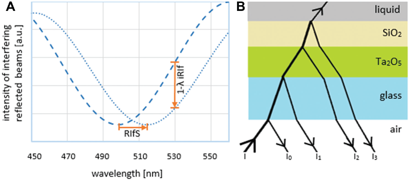
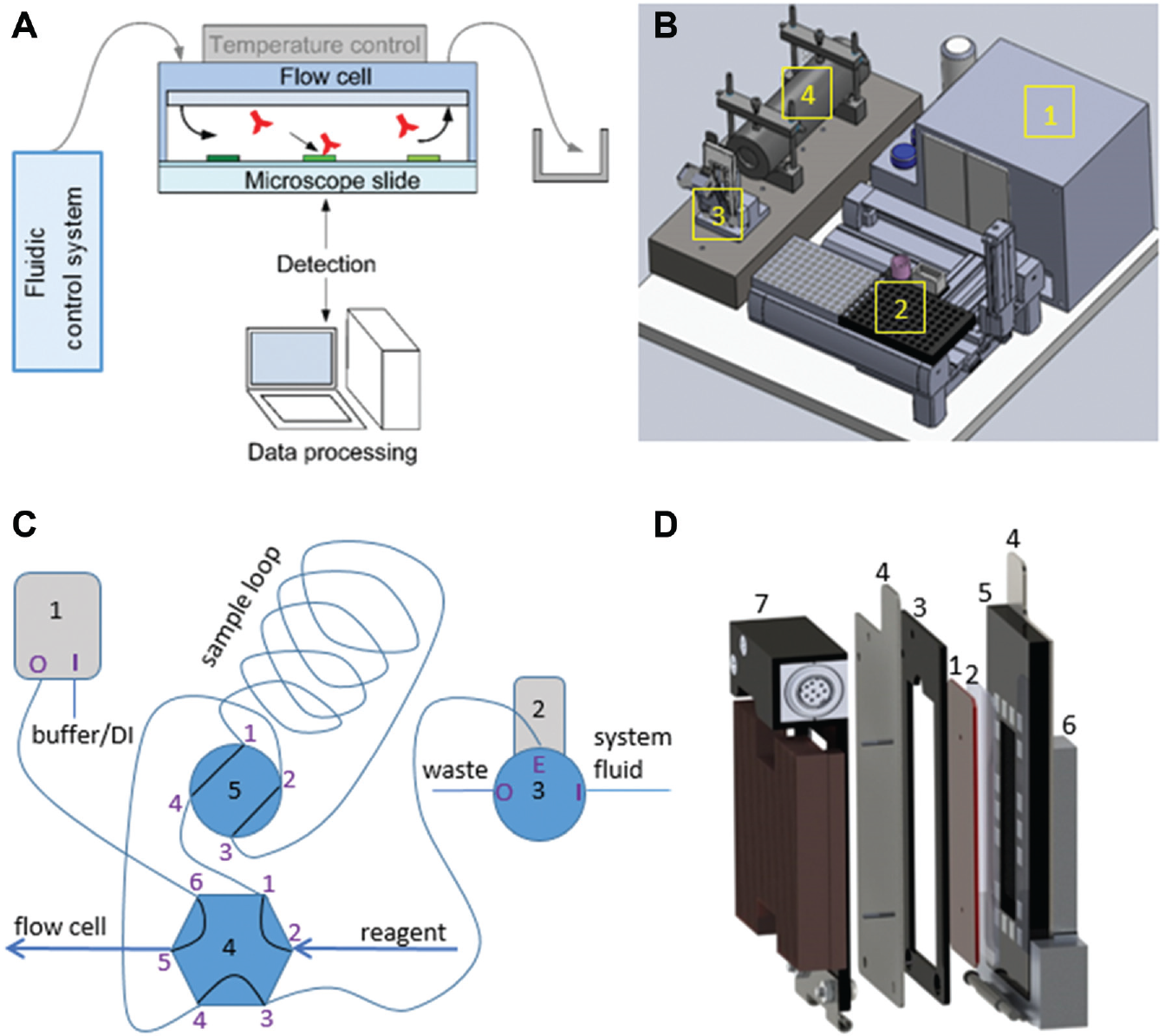
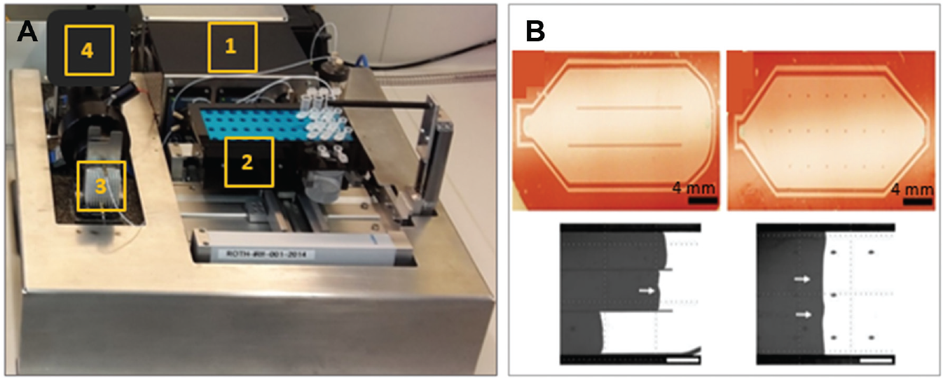
The presented setup consists of four hardware components: the generic microfluidic flow cell with temperature controller, the fluidic system, the optical detection unit, and the hardware for system controlling, data acquisition, and data processing ( Fig. 2A ). The main arrangement of the components considers the short length of the tubes for minimizing the dead volumes ( Fig. 2B and Fig. 3A ). On the right rear side, the electrically controlled fluidic system (1) with the housing for a Vici Pump M6 (VICI AG International, Schenkon, Switzerland), a Hamilton syringe pump PSD/4, one Hamilton MVP 6-port, and one Hamilton MVP 4-port loop valve is implemented (Hamilton Company, Reno, NV, USA). This housing further serves as electrical cabinet for the temperature controller, the LED current control, and the voltage supply. In front of this cabinet, there is a sampler (2) made of a Festo (Brussels, Belgium) EXCM x-y module (150 × 110 mm) cooled by Peltier elements and the Festo CMMO vertical axis (40 mm). Left to the sampler, there is the microfluidic flow cell (3) mounted onto a damped stone plate that further fixes the optical detection system—a CMOS camera and a telecentric lens system (4). The design of the fluidic system ( Fig. 2C ) follows the idea of having a constant flow of different reagents or buffer through the flow cell. While buffer is dispensed, the next reagent sample is aspirated into the sample loop. While priming the reagent into the flow cell, the reagent sampling tip is washed to avoid cross-contamination. The system allows having sample volumes of up to 1100 µL and continuous flow rates of 5 nL/min to 5 mL/min. Samples are aspirated into the sample loop by the Hamilton PSD/4 syringe pump with a 2.5-mL syringe. The modular valve positioners (MVP) valves control the fluidic flows. In mode 1, the Vici is pumping buffer through the flow cell while the PSD/4 first washes the sample loop with buffer taken via valve port 3I, then aspirates the next reagent into the sample loop. From sampler tip to sample loop, there is a total dead volume of ~40 µL. In mode 2, both valves turn one step to the right. Now the Vici pump dispenses into valve port 4.6, out through port 4.1 and into valve port 5.4, out through 5.3 via the sample loop and into 5.1, out through 5.2 and into 4.4, and out through 4.5 and into the flow cell. By changing the flow direction from aspirating to dispensing the reagent, Taylor dispersion and cross-contamination are minimized. To avoid contamination after each reagent step, the sample loop is cleaned by a washing procedure. Sample loop and tubings are washed by pumping 1.2 mL (programmable volume) of buffer through the system into the washing stations waste (50-mL standard tube).

Figure 2.

(A) Schematic of the imaging reflectometric interferometry (iRIf) system setup: fluidic control system, microfluidic flow cell with temperature controller, optical detection system and PC for system controlling, sensor data acquisition, and processing. (B) Arrangement of iRIf system components, fluidic control system (1), reagent sampler (2), microfluidic flow cell (3), and optical detection system (4) resulting in low dead volumes and portable system of a maximum of 25 kg. (C) Fluidic system for constant flow of different reagents or buffer through flow cell. While buffer is dispensed, the next reagent sample is aspirated. Low Taylor dispersion in sample loop due to change of flow direction from aspiration to dispensation. (D) Flow cell handheld consisting of PDMS inlay (1) and glass slide (2) in a standard format of 75 × 25 mm², frame for PDMS inlay (3), ferromagnetic metal sheets (4), magnets frame (5), backbone (6), and Peltier elements with cooler (7). Design allows for defined, highly parallel clamping at low pressure such that flow cell height is kept parallel across the whole chamber area. Peltier tempers between 15 °C and 50 °C.

Figure 3.

(A) Imaging reflectometric interferometry (iRIf) system setup: (1) electrical cabinet for power supply, LED current controller, temperature controller for rack and flow cell, controllers and mechanics of Vici pump M6, Hamilton PSD/4 syringe pump, Hamilton MVP 4-port loop and 6-port loop valve; (2) sampler for 33 × 500–µL tubes and 11 × 1.5–mL tubes mounted on Festo EXCM x-y stage, range of 150 × 110 mm, cantilever for sampling tube on Festo CMMO z-axis, range of 40 mm; (3) flow cell handheld; and (4) optical detection unit with camera and telecentric lens system. (B) Priming analyses of PDMS flow cells with support structures; for example, (left) support lanes and (right) trapezoidal support pillars show disadvantages of the lane type due to inhomogeneous priming (bottom).

The microfluidic flow cell is mainly made of a structured PDMS slide in a 75 × 25–mm² format with a thickness of 1 mm and a sealing glass slide in the size of a standard microscope slide. The PDMS slide is molded in a centrifuge (3T Analytics, Tuttlingen, Germany) with a structured Si wafer as the master. The Si wafer is structured by lamination (laminator Mylam 12; 105 °C; rest time, 20 min) of dry-resist Ordyl SY300¹⁹ of 30 µm or (2×) 20 µm thickness followed by a photo-lithography process (exposure time, 11 s; postbake at 85 °C for 1 min; hard bake developing at 105 °C for 60 min). Finally, the structured wafer is silanized in a dessicator with trichlorosilane (25 µL on glass slide; 10-s vacuum; incubation, >6 h; postbake at 90 °C for 1 h).

The sandwich of PDMS and the glass slide needs a well-defined clamp—with a defined pressure and highly parallel to prevent the flow cell chamber from being deformed or distorted. A magnetic clamping system ( Fig. 2D ) using 5-mm³ square-shaped magnets patterned by a laser-cut PMMA template allows for a constant flow cell height across the whole chamber area such that flow rates remain homogeneous. Quick and easy exchange of the flow cell is realized by a hinge design. Rather thin ferromagnetic stainless plates with a monitoring window shape the backbone, but they allow the dynamic tempering of the flow cell by a Peltier element (40 × 20 mm², 8 A maximum) between 15 °C and 50 °C. Laser-welded inlet and outlet tube pins through the front plate connect the flow cell to the fluidic system.

The detection unit consists of four major elements: a digital camera (5 megapixel), a telecentric lens system, a 530-nm LED as the light source, and a high-precision LED current controller. As such, the system allows a spatial resolution of ~7 µm on the microarray of size ~18 × ~15 mm.

Both the surface structures and the inlet/outlet geometries of the PDMS inlay are optimized to improve sealing, priming, and overall easy and robust handling/assembling. The priming behavior of different structures is analyzed. Due to the low height of 30 (40) µm of the flow cells’ main chamber in comparison to its surface of ~30 × 15 mm², structures such as lanes or trapezoidal pillars to avoid collapsing are especially investigated ( Fig. 3B ).

A process controller programmed in C# runs the setup with a standard PC. It controls all compounds via serial-to-USB interface (pumps, valves, temperature controllers) or via TCP/IP interface (Festo axes). Complex process protocols can be edited or programmed by skilled users in a simplified C code being interpreted at runtime. For standardized protocols, parameters can be loaded from an Excel chart.

While the fluidic protocol is running, the camera observes the reflected interference signal. The image-processing interface allows one to view the original camera picture in a live view mode or the referenced quotient picture sequence in a live view iRIf mode. Intensity changes are enhanced visually by a look-up table that is typically set to a maximum for 5% signal change.

For the quantification of the binding kinetics, time-resolved binding curves are calculated. Each spot of interest and an according local background are identified manually or by a spot identification routine programmed in MATLAB (MathWorks, Natick, MA). For each frame, the mean pixel intensities of the spots are divided by the mean intensities of their local backgrounds for normalization. Any two of these normalized values can now be divided by each other to get the relative spot intensity, which is the mean intensity change of spot pixel values from time t₁ to time t₂:

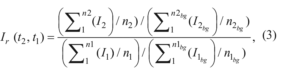
I_{r} (t_{2}, t_{1}) = \frac{(\sum_{1}^{n 2} (I_{2}) / n_{2}) / (\sum_{1}^{n 2_{b g}} (I_{2_{b g}}) / n_{2_{b g}})}{(\sum_{1}^{n 1} (I_{1}) / n_{1}) / (\sum_{1}^{n 1_{b g}} (I_{1_{b g}}) / n_{1_{b g}})},

where

I_{r} (t_{2}, t_{1}) = mean intensity change from t_{1} to t 2_{} of normalized spot

I_{1}, I_{2,} I_{1 b g}, I_{2 b g} = pixel intensities at times t_{1} and t_{2}

n_{1}, n_{2}, n_{1 b g}, n_{2 b g} = number of pixels of data and background spots

For increasing the signal-to-noise ratio (SNR) by reducing noise (e.g., shot noise²⁰), a median reference picture can be calculated from a range of frames.

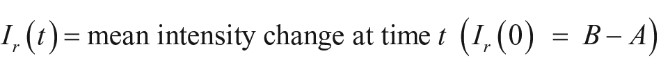
To determine the binding coefficient KD, an exponential function is fitted to each binding curve^21–23 by a MATLAB program based on the least squares fitting method.²⁴ By this function, the observable binding rate constant kobs can be calculated:

I_{r} (t) = B - A * e^{- k o b s * t},

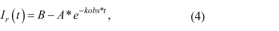
where

I_{r} (t) = mean intensity change at time t (I_{r} (0) = B - A)

B = y shift

A = scaling factor

k o b s = observable rate constant

For the determination of kobs, only the middle part of a binding can be used, since before we have a diffusion limitation and later we have biexponential behavior caused by both associations and increasing dissociations. This middle part is depicted by plotting the signal derivative over the signal and selecting the linear region.

\frac{\frac{d I_{r} (t)}{d t}}{I_{r} (t)} .

Having determined kobs of at least two different reagent concentrations, we can calculate ka and kd; as an alternative, kd could be seized by a dissociation experiment, and then only one concentration would be required for the calculation of ka:

k o b s = k a * c + k d,

where

k a, k d = association and dissociation rate constant

c = reagent concentration

Finally, the dissociation constant KD can be calculated by

K D = \frac{k d}{k a} .

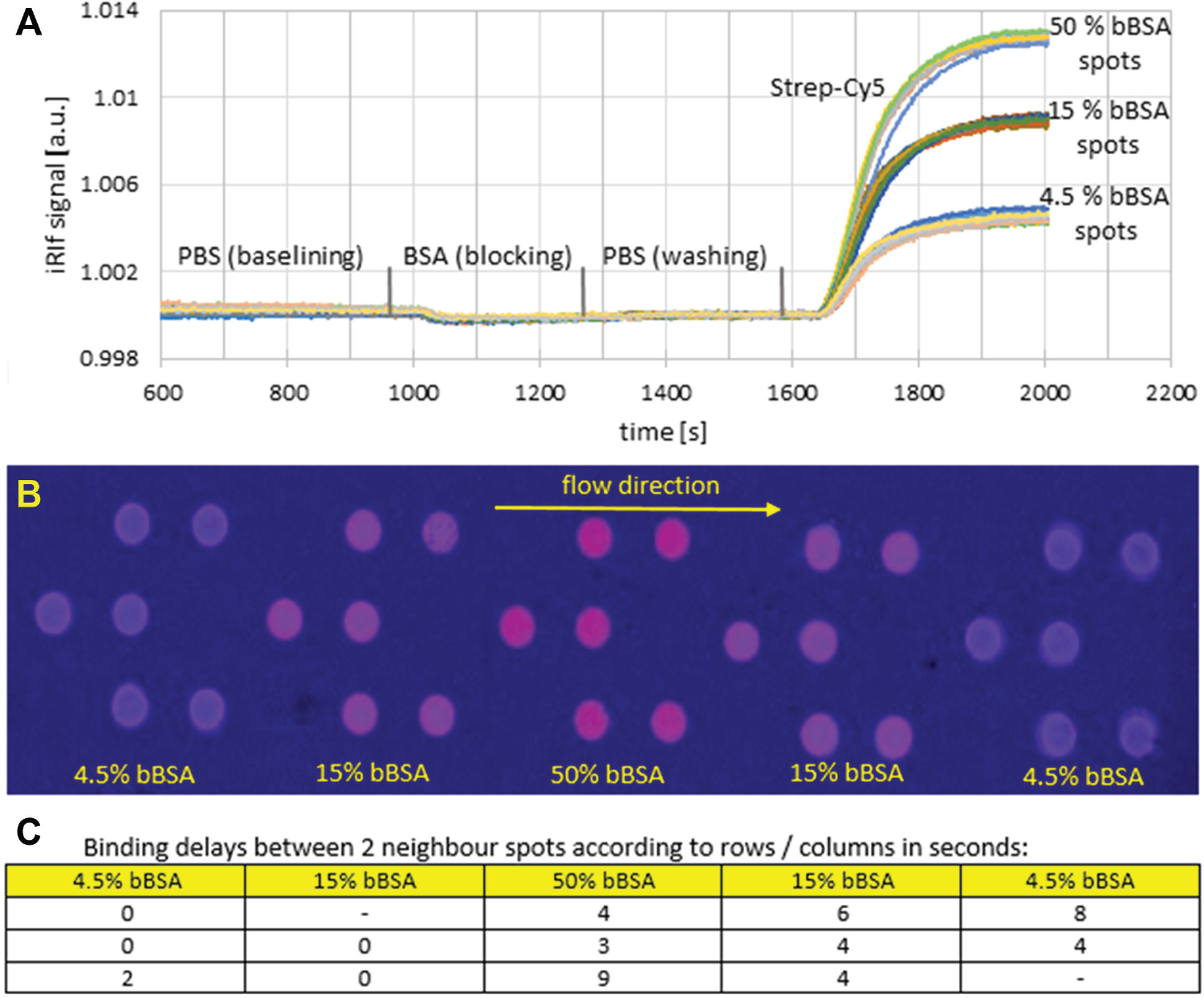
Materials for biotinylated bovine serum albumin (bBSA) streptavidin binding analysis ( Fig. 4 ): microarrays of the bBSA fraction (V) in four volumes (0.7, 2.1, 6.3, and 18.9 nL/spot) and three concentrations (4.5%, 15%, and 50%) were spotted onto microscope glass slides with reflective thin film layers (Ta₂O₅ [10 µm]/SiO₂ [330 µm]), silanized with (3-glycidyloxypropyl)trimethoxysilane (GOPTS), and incubated for 1 h after O₂ plasma activation for 4 min. bBSA spots were incubated more than one night at 4 °C in a humid (1× phosphate-buffered saline [PBS], pH 7.2) environment. Flow injection was analyzed with a sequence of buffer, BSA, buffer, streptavidin-Cy5, and buffer, each at 60 µL/min for 5 min. PBS (pH 7.2) was used as a buffer, with BSA at 5 mg/mL and streptavidin at different concentrations of 0.5, 1, 2, 5, and 10 µg/mL.

Figure 4.

(A) Binding curve determination for slide 022, spots with a volume of 6.3 nL, by the Java method. After baselining with phosphate-buffered saline (PBS) (960 s), bovine serum albumin (BSA) is used for blocking (300 s), followed by a PBS washing step (300 s) and streptavidin-Cy5 (2 µg/mL), each being primed with a flow rate of 60 µL/min. Each set of spots with equal biotinylated bovine serum albumin (bBSA) concentrations (50%, 15%, 4.5%) creates a set of curves. (B) Quotient picture of 2 µg/mL streptavidin-Cy5 bound to bBSA array spots of 6.3 nL, from left to right concentration clusters (each six spots) of 4.5%, 15%, 50%, 15%, and 4.5% bBSA in BSA. (C) Analysis of normalized curve shifts at inflexion points related to spot positions; spots in proximity to each other (distance of 1 mm) see delays of up to 9 s while only ~0.5 s would be expected with a flow rate of 60 µL/min, which is a flow rate vector of 2.22 mm/s. Hence, other reasons cause the additional delay (e.g., depletion of the reagent in diffusion layer, local inhomogeneities of flow cell geometry, or surface coating).

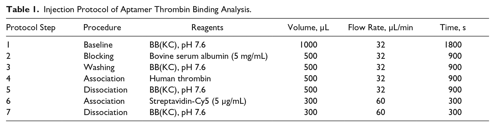
Materials for aptamer thrombin binding analysis ( Fig. 6 ): fibrinogen binding site aptamers elongated with a T20 spacer²⁵ at a concentration of 15 µM were spotted in volumes of 2.1 nL/spot onto microscope glass slides with reflective thin film layers (Ta₂O₅ [10 µm]/SiO₂ [330 µm]), activated with the homobifunctional linker PDITC.²⁶ Aptamer spots were incubated more than one night and protected from light in a humid (1× PBS, pH 7.2) environment. Spotted slides were immersed for 30 min in 10% ethanolamine, flushed with (distilled) water, immersed two times for 5 min in preheated (70 °C) DI water, and then blocked with 10 µg/mL BSA in PBS for 15 min. The flow injection protocol was defined according to Table 1 .

Table 1.

Injection Protocol of Aptamer Thrombin Binding Analysis.

Protocol Step	Procedure	Reagents	Volume, µL	Flow Rate, µL/min	Time, s
1	Baseline	BB(KC), pH 7.6	1000	32	1800
2	Blocking	Bovine serum albumin (5 mg/mL)	500	32	900
3	Washing	BB(KC), pH 7.6	500	32	900
4	Association	Human thrombin	500	32	900
5	Dissociation	BB(KC), pH 7.6	500	32	900
6	Association	Streptavidin-Cy5 (5 µg/mL)	300	60	300
7	Dissociation	BB(KC), pH 7.6	300	60	300

All arrays were spotted with the Scienion (Berlin, Germany) sciFLEXARRAYER S3/S5²⁷ provided by the chair of Chemistry and Physics of Interfaces (CPI), IMTEK, University of Freiburg.

Results and Discussion

Technical-Physical Analysis

Thirty iRIf glass slides were spotted in total with 120 bBSA spots/slide and assembled with a PDMS flow cell of the trapezoidal pillar type. A sequence of experiments with streptavidin-Cy5 concentrations of 0.5, 1, 2, 5, and 10 µg/mL was run, leading to the results depicted in Figure 4 . The reference picture was set within the second PBS step, with the concentrations series of bBSA clearly visible. Next we automatically identified the spots via MATLAB²⁴—median filtering (medfilt2), binary pic conversion (im2bw) with global thresholding (graythresh), oval-shaped region of interest (ROI) identification (regionprops), and determination of local backgrounds. Then a Java routine calculated the binding curves of each spot ( Fig. 4A ) (e.g., experiment no. JB100_S187(22), 6.3 nL spots). The curves started with the PBS baselining for 960 s. Next came BSA (5 mg/mL) for 300 s; it slightly bound to the background as desired. After washing with PBS for another 300 s, we primed 2 µg/mL streptavidin-Cy5. Each concentration of bBSA spots (4.5%, 15%, 50%) created a bundle of curves, with relative intensity increasing by ~0.4% for each concentration. Within each set of curves, we had an intensity variation at the end point of ~0.05%; the variation for the lowest concentration of 4.5% was slightly higher. Curve shifts related to spot positions are depicted as time delays at the inflexion points of normalized curves in Figure 4C . Spots in proximity of each other should see the same flow rate due to the very high ratio of flow cell width/flow cell height of 500 (width of ~15 mm, height of ~30 µm); the parabolic flow profile is expected only within the first 50 µm from the side walls.²⁸ However, we saw significant binding delays of up to 9 s for spots at a distance of 1 mm. A flow rate of 60 µL/min led to a flow rate vector in the flow cell of 2.22 mm/s.

v_{f c} = \frac{v_{s y s}}{f c_{w *} f c_{h}} / 60,

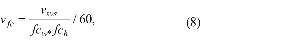
where

v_{f c} = flow vector in flow cell in mm / s

v_{s y s} = flow rate in µ L / \min

f c_{w}, f c_{h} = flow cell width and height in mm

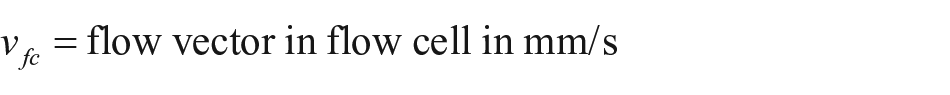
For a spot distance of 1 mm, that would make a binding delay of only ~0.5 s. Hence, the significantly higher binding delays as measured are not only caused by the flow vector but also by depletion of the reagent due to limited diffusion. Local inhomogeneities of flow cell geometry and surface coating could be further reasons for irregular time shifts.

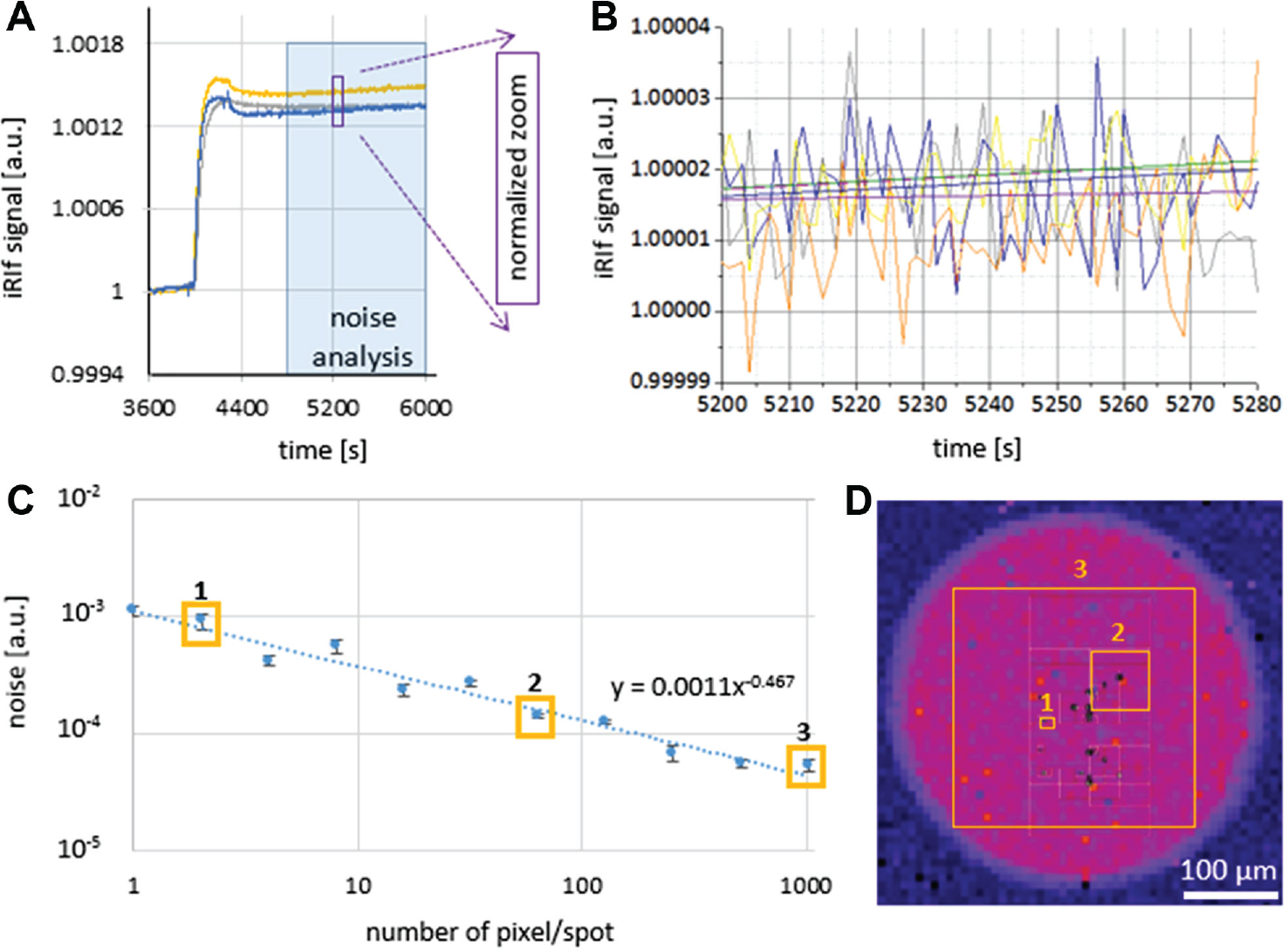
By a bBSA streptavidin assay (PBS, BSA, PBS, streptavidin, PBS, with each PBS step for 30 min and the others for 5 min at 60 µL/min), we quantified noise and drift. We started to analyze the curves 10 min after the final streptavidin washing step began, that is, from time 4800 s to 6000 s ( Fig. 5A ). Each curve was normalized with its initial data at time 4800 s ( Fig. 5B ). We saw a baseline drift of <0.0003%/min and a random noise of 0.003%. Possible minimization of spots was analyzed next. Noise increased upon the function 1/pn^1/2 (pn = spots pixel no.). If spatial averaging is calculated for noise filtering only, a spot size of more than 200 pixels is recommended ( Fig. 5C ).

Figure 5.

(A) Quantification of noise based on biotinylated bovine serum albumin (bBSA) streptavidin assay (JB113_S106(2)) with three manually spotted bBSA spots of 50%. Analysis starts 10 min after beginning the final washing step from 4800 s to 6000 s. (B) Each curve is normalized with its initial data at time 4800 s, leading to baseline drift of <0.0003%/min and random noise of 0.003%. (C) Noise level essentially depends on the size of the observed spot. Noise reduces by ~1/pixel no.^1/2, and a spot size of >200 pixels (~14 × 14 pixels or diameter of ~16 pixels [~110 µm]) is recommended. (D) Data depicted from experiment JB100_S187(22), spot 13, phosphate-buffered saline (PBS) washing before streptavidin binding from time 1300 s to 1600 s with spots of 4 × 1 pixels, 4 × 2 pixels, 2 × 4 pixels, 2 × 8 pixels, 2 × 16 pixels, 2 × 32 pixels, 2 × 64 pixels, 2 × 128 pixels, 1 × 256 pixels, 1 × 512 pixels, and 1 × 1024 pixels according to rectangular spot regions of interest (ROIs) (e.g., one ROI for each of 1024, 64, and 2 pixels is highlighted).

All hardware components of the tempering and fluidic systems are controlled by a user interface programmed in C#, open to any new components. The user can easily create a fluidic protocol by simply entering parameters such as flow rate, priming time, and flow cell temperature for each assay step into an Excel chart or by writing an individual protocol with a specific editor. The monitoring and data processing are based on an open Java code using ImageJ (National Institutes of Health, Bethesda, MD) features and MATLAB. Routines for median filtering, quotient pictures, movies, semiautomated spot identification, binding curves, and finally KD determination are provided. This setup enables the user to perform sensitive label-free binding analysis on microarray spots within a robust and easy-to-operate environment. Open SW modules allow the permanent optimization of routines and the system expansion.

Biochemical Analysis

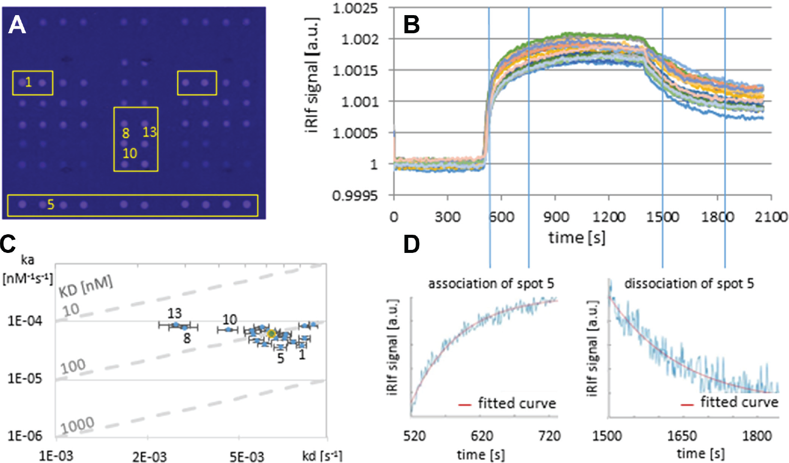
Next we proved the suitability of the system for biological binding analyses. For a first KD value determination, we applied thrombin of different concentrations (1.33, 2, 3, 4.5, 6.7, and 10 µg/mL = 35.8, 53.7, 80.5, 120.7, 181, and 272 nM) to spotted fibrinogen binding site aptamers elongated with a T20 spacer.²⁵ We evaluated the binding at various positions ( Fig. 6A ) and determined the association and dissociation curves as described before ( Fig. 6B ). Scatterplots visualized the quality of each fit of association and dissociation ( Fig. 6D ), resulting in an average dissociation constant KD of 101 nM with individual values of 32 to 208 nM ( Fig. 6C ), which matches the reported KD of typical thrombin aptamer bindings of 25 to 200 nM.²⁹

Figure 6.

(A) Array of eight different aptamers having bound thrombin and 20 spots of fibrinogen binding site aptamer elongated with a T20 spacer (A14, framed yellow). (B) Association of thrombin to A14 followed by dissociation; evaluable region for association determined by time 520 s to 750 s; for dissociation, time 1500 s to 1850 s. (C) Blue dots cloud depicting KD values (dissociation rate constant kd/association rate constant ka) with average KD of 101 nM (orange dot); “irregular” values (e.g., 8, 10, and 13 with lower KD or 1 and 5 with higher KD) occurred. (D) Fitting of exponential functions to the evaluable regions of the binding curves, for example, dissociation (right) and association (middle) of spot 5.

Total preparation time for slide surface coating, spotting, and blocking summed up to 2 to 3 days for up to 50 slides. Slides spotted with bBSA or aptamers could be stored at 4 °C for >1 week. Flow injection analysis commonly takes 1 to 2 hours per slide for standard injection protocols. Applying the Scienion sciFLEXARRAYER S3/S5 for array spotting onto GOPTS- or PDITC-coated microscope slides with spot numbers of ~1000 and volumes of 0.7 nL/spot could be realized, resulting in spot diameters of ~0.2 mm. Donut effects were reduced with increasing reagent concentration and decreasing spot size.

Outlook

An automated setup for label-free real-time imaging and analysis of binding interactions based on the 1λ-iRIf system was realized. The optical system with a green LED of 530 nm detects intensity signal changes of <10⁻⁴ by spatial averaging of ~200 pixels ( Fig. 5C ), such that it is competitive with BIAcore systems.³⁰ A generic microfluidic flow cell system based on micro-structured PDMS inlays in a standard microscope slide format was realized and proved its validity for flow injection analysis. Versatile microstructures and flow cell heights allow for individual process optimization, a magnetic clamping system provides robust and quick flow cell exchange, and optical properties such as high absorption of the red PDMS allow for low system noise caused by noncoherent reflections. Low dead volumes both in tubes and valves as well as in the microfluidic flow cell of ~50 µL allow reagent volumes of less than 300 µL. The technical-physical analysis revealed reagent depletion potentially affecting the KD determination. That needs to be addressed while designing the spotting pattern. Random noise of <5 × 10⁻⁵ and a baseline drift of <3 × 10⁻⁶/min allow sensitive long-term measurements. The system proved to be valid for biochemical analyses, too. By analyzing aptamer-protein interactions, KD values close to published ones could be determined.

Multistep enzyme-linked immunosorbent assay–like interactions on antigen arrays with several antibodies revealed the system’s potential in microarray-based kinetic data acquisition ( Fig. 7 ). Basic analyses of immunizations of rabbit sera indicated possibilities for applications in vaccine verification.

Figure 7.

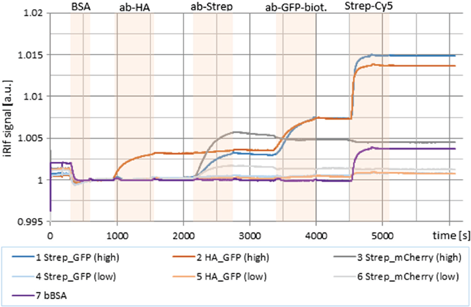
Multistep assay based upon three proteins in two concentrations (50 µg/mL = high; 5 µg/mL = low) + biotinylated bovine serum albumin (bBSA) as a positive control spotted onto a 1,4-phenylene diisothiocyanate (PDITC)–coated glass slide. BSA binds to background as desired. ab-HA binds to HA_GFP, ab-Strep binds to Strep_GFP and Strep_mCherry, biotinylated ab-GFP binds to GFP spots, and streptavidin binds to biotinylated ab-GFP and to bBSA as a positive control. GFP, green fluorescent protein; HA, human influenza hemagglutinin.

By technical means, the system throughput could be further expanded. The camera resolution of >5 million pixels for an image size of ~18 × 15 mm² enables one to monitor simultaneously >10,000 spots at sizes of 200 pixels, that is, ~110 µm in spot diameter. Even more spots of lower size could be detected by pixel intensity averaging or median value determination over time, but enhanced microarray formation technology would be required.³¹

Footnotes

Acknowledgements

We are grateful to Biametrics, Tübingen, for supporting us with their iRIf technology expertise and Holger Frey, IMTEK, Freiburg for spotting of microarrays.

Declaration of Conflicting Interests

The authors declared no potential conflicts of interest with respect to the research, authorship, and/or publication of this article.

Funding

The authors disclosed receipt of the following financial support for the research, authorship, and/or publication of this article: The research leading to these results has received funding from the German Ministerium für Wissenschaft, Forschung und Kunst Baden-Württemberg within project Ideenwettbewerb Biotechnologie und Medizintechnik, PTJ 33-720.830-6-52; the German BMBF within e:bio project ReelinSys FKZ 0316174; and the European Union within the FP7 innovation funding project CE microarray, grant number 606618.

References

Fechner

Bleher

Ewald

. Size Does Matter! Label-Free Detection of Small Molecule-Protein Interaction. Anal. Bioanal. Chem. 2014, 406, 4033–4051.

Malmqvist

Biospecific Interaction Analysis Using Biosensor Technology. Nature 1993, 361, 186–187.

3T Analytik. Quartz Crystal Microbalances. http://www.3t-analytik.de/ (accessed April 4, 2016).

ForteBIO. Octet RED96 System. http://www.fortebio.com/ (accessed April 4, 2016).

Homola

Yee

S. S.

Gauglitz

Surface Plasmon Resonance Sensors: Review. Sens. Actuators, B 1999, 54, 3–15.

Gauglitz

Direct Optical Sensors: Principles and Selected Applications. Anal. Bioanal. Chem. 2005, 381, 141–155.

Gauglitz

Brecht

Kraus

. Chemical and Biochemical Sensors Based on Interferometry at Thin (Multi-) Layers. Sens. Actuators, B 1993, 11, 21–27.

Proll

Markovic

Steinle

. Reflectometric Interference Spectroscopy. Methods Mol. Biol. 2009, 503, 167–178.

Pröll

Möhrle

Kumpf

. Label-Free Characterisation of Oligonucleotide Hybridisation Using Reflectometric Interference Spectroscopy. Anal. Bioanal. Chem. 2005, 382, 1889–1894.

10.

Gauglitz

Point-of-Care Platforms. Annu. Rev. Anal. Chem. 2014, 7, 297–315.

11.

GE Healthcare. Handbook BR-1006-47 Edition AD. 2007, No. 1, 1–82. http://www.iata.csic.es/IATA/usct/geno/Doc/Docu%20Equipamiento/T100%20Instrument%20Handbook%202007.pdf (accessed January 27, 2015).

12.

Mateescu

Wang

Dostalek

. Thin Hydrogel Films for Optical Biosensor Applications. Membranes 2012, 2, 40–69.

13.

Ewald

Entwicklung und Charakterisierung einer portablen Biosensorplattform zur markierungsfreien Multi-Analyt-Bestimmung. Dissertation, Eberhard-Karls-Universität Tübingen, Tübingen, 2014.

14.

Frank

Reflektometrische und integriert optische Sensoren für die Bioanalytik. Dissertation, Eberhard-Karls-Universität Tübingen, Tübingen, 2005.

15.

Markovic

Einsatz von Nanopartikeln und optimierten Schichtsystemen für die Signalverstärkung in reflektometrischen Biosensoren. Dissertation, Eberhard-Karls-Universität Tübingen, Tübingen, 2008.

16.

Sun

Y.-S.

Use of Microarrays as a High-Throughput Platform for Label-Free Biosensing. J. Lab. Autom. 2015, 20, 334–353.

17.

Bleher

Schindler

Yin

M.-X.

. Development of a New Parallelized, Optical Biosensor Platform for Label-Free Detection of Autoimmunity-Related Antibodies. Anal. Bioanal. Chem. 2014, 406, 3305–3314.

18.

Pröll

iRIfS-imaging Reflectrometric Interference Sensor: ein System für die hochparallele und markierungsfreie Untersuchung biomolekularer Wechselwirkungen. Dissertation, Eberhard-Karls-Universität Tübingen, Tübingen, 2010.

19.

Elga Europe. Data Sheet ORDYL SY 300. file://C:/Users/juergenb/Downloads/PRODUCT_DATA_SHEET_SY300.PDF.PDF (accessed April 5, 2016).

20.

Tyson

ShotNoise.dvi. http://123.physics.ucdavis.edu/shot_files/ShotNoise.pdf (accessed March 4, 2015).

21.

Karlsson

Michaelsson

Mattsson

Kinetic Analysis of Monoclonal Antibody-Antigen Interactions with a New Biosensor Based Analytical System. J. Immunol. Methods 1991, 145, 229–240.

22.

Gauglitz

Reichert

Affinitätsreaktionen: Beschreibung von Immunoassays, Testformaten, Massentransport, Bind-ungskinetik. http://www.chemgapedia.de/vsengine/vlu/vsc/de/ch/13/vlu/kinetik/affinitaet/affinitaetsreaktionen.vlu/Summary.html (accessed March 2015).

23.

Laenge

Einsatz der Fließ-Injektions-Analyse in markierungsfreien Bindungsassays. Dissertation, Eberhard-Karls-Universität Tübingen, Tübingen, 2000.

24.

MathWorks. Least-Squares Fitting—MATLAB; MathWorks: Natick, MA, 2014.

25.

Balamurugan

Obubuafo

McCarley

R. L.

. Effect of Linker Structure on Surface Density of Aptamer Monolayers and Their Corresponding Protein Binding Efficiency. Anal. Chem. 2008, 80, 9630–9634.

26.

Hoffmann

Hin

Stetten

F. v.

. Universal Protocol for Grafting PCR Primers onto Various Lab-on-a-Chip Substrates for Solid-Phase PCR. RSC Adv. 2012, 2, 3885.

27.

Wulfetange

Scienion Enabling Life Science- sciFLEXARRAYER Ultra-Low Volume Dispensers. http://www.scienion.com/fileadmin/user_upload/pdf/11_sciFLEXARRAYER_SX_20140903.pdf (accessed March 4, 2015).

28.

Meyer

P. A.

Design and Characterization of Microfluidic Flow Cells for Label-Free Reflectrometric Analysis of Molecular Binding Kinetics. Master’s thesis, Albert-Ludwigs-Universität Freiburg, Freiburg, 2014.

29.

Bock

Griffin

L. C.

Latham

J. A.

. Selection of Single-Stranded DNA Molecules That Bind and Inhibit Human Thrombin. Nature 1992, 355, 564–566.

30.

GE Healthcare Life Sciences. Biacore T200. Data file 28-9794-15 AB. 2015. http://www.gelifesciences.co.jp/catalog/pdf/28979415ab.pdf (accessed June 15, 2015).

31.

Hoffmann

Trotter

Stetten

F. v.

. Solid-Phase PCR in a Picowell Array for Immobilizing and Arraying 100 000 PCR Products to a Microscope Slide. Lab Chip 2012, 12, 3049.

Low-Volume Label-Free Detection of Molecule-Protein Interactions on Microarrays by Imaging Reflectometric Interferometry

Abstract

Keywords

Introduction

Materials and Methods

Results and Discussion

Technical-Physical Analysis

Biochemical Analysis

Outlook

Footnotes

Acknowledgements

Declaration of Conflicting Interests

Funding

References