Applying Dataflow Architecture and Visualization Tools to In Vitro Pharmacology Data Automation

Abstract

The pace and complexity of modern drug discovery places ever-increasing demands on scientists for data analysis and interpretation. Data flow programming and modern visualization tools address these demands directly. Three different requirements—one for allosteric modulator analysis, one for a specialized clotting analysis, and one for enzyme global progress curve analysis—are reviewed, and their execution in a combined data flow/visualization environment is outlined.

Introduction

The pace and complexity of modern drug discovery places ever-increasing demands on scientists and calls for analysis and visualization tools that can adapt quickly, simplify the understanding of complex data sets, and, at the same time, maintain analytical and scientific consistency with foundational work. Data flow programming and modern visualization tools address these demands directly. Data flow programming environments provide a platform to build on existing, validated data analyses; minimize manual operations; and deploy new and revised work flows quickly. Modern visualization tools provide an immediacy of data digestion that speeds process development and adoption as well as improves data understanding once a solution is in place.

The general requirement addressed here is analyzing, modeling, and annotating instrument data for visualization and downstream transfer to general biological data databases. The specialized analyses here were developed for cases that were not well addressed by existing standard methods. The analyses use data files from different laboratory instruments but share a programming environment, a curve-fitting tool, and a customizable visualization tool. Three different requirements—one for allosteric modulator analysis, one for a specialized clotting analysis, and one for enzyme global progress curve analysis (GPCA)—are reviewed, and their execution in a combined data flow/visualization environment is outlined.

Informatic Methods

The primary programming environment for this work was Biovia Pipeline Pilot (PLP),^1,2 a data flow programming environment characterized by graphical connection of custom and predefined components. Within PLP, tabular input data move row by row through graphs of connected processing nodes. Node checkpoints can be set to save complete row results up to that processing node. The saved or cached data allow changes to be made downstream of the checkpoint node, and then processing can restart from that node without time-consuming reexecution of already completed parsing and analysis upstream of the checkpoint node. This can save significant time, particularly in finalizing the output details of a lengthy process. In addition, PLP has standard components for file reading, statistics, caching, database access, and filtering that enable the addition of routine and even complex functionality to a script very easily. Together, the Pipeline graphical architecture and its component libraries form a programming tool kit well suited to the tasks of data analysis automation such as reading and parsing data files, creating subsets for modeling, and reassembling model results with the original data set.

The customizable visualization tool used for this work is TIBCO Spotfire 5.51. ³ Spotfire has its roots in work in the 1990’s at the University of Maryland Human-Computer Interaction Lab. ⁴ Ben Schneiderman summarized the underlying elements of Spotfire with a “Visual Information Seeking Mantra: Overview first, zoom and filter, then details-on-demand.” ⁵ Spotfire has varied visualizations, but the real power comes from dynamic querying—selecting what is viewed—that makes a Spotfire file open to exploration. ⁶

The curve-fitting tool critical to this work was GraphPad Prism 6.0, which is an industry-standard tool for curve fitting of pharmacologic data. ⁷

Case 1: Global Curve Fitting for Allosteric Modulators

Background

The first case considers the development of data-modeling automation for allosterism analysis. Allosteric receptor modulators are of growing interest as novel pharmacologic entities owing to their potential for enhanced safety and selectivity.^8,9 Allosteric modulators can be positive allosteric modulators, which act to enhance the response of a receptor to an agonist, or negative allosteric modulators, which decrease a receptor’s response to an agonist. Given an assay for agonist activity, an allosteric compound can be characterized by running the assay across a dual titration so that each compound concentration in a titration series is tested in combination with a full titration of the reference agonist. The resulting activity matrix or response surface can then be modeled with the general operational model, which uses eight fit parameters that are globally shared (but preferably some or all of the agonist-specific parameters should be properly constrained) across the matrix of activities. ¹⁰ See Figure 1 for the general governing equation. When chi is set to 0, that is, when the basal level activity is absent, a less general model that does not have the chi parameter may be used. ¹¹ In our lab, to characterize one compound, we typically use a matrix of 160 wells created by combining 16 concentrations of the allosteric modulator with a 10-point titration of the receptor agonist. The seven or eight parameters of global curve fit and its 160 wells are in contrast to the four-parameter logistic fit and 10-well dose titration used to characterize a wide range of pharmacology targets for both antagonism and agonism. The coverage of the full dynamic range of both chemical entities—agonist and modulator—is often visualized as a succession of agonist dose-response curves performed at varying test compound concentrations. Considered either as a matrix or as a succession of curves, the constituents of the wells tested are the same. See Figure 2 for a three-dimensional (3D view of a negative allosteric modulator response surface.

Figure 1.

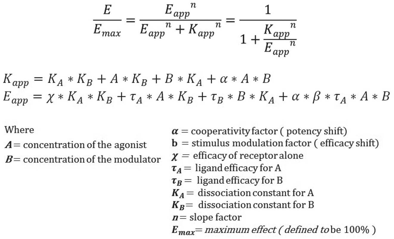
General equation for allosterism. This version of the general equation for allosterism includes modeling of constitutive receptor activity using the chi parameter.

Figure 2.

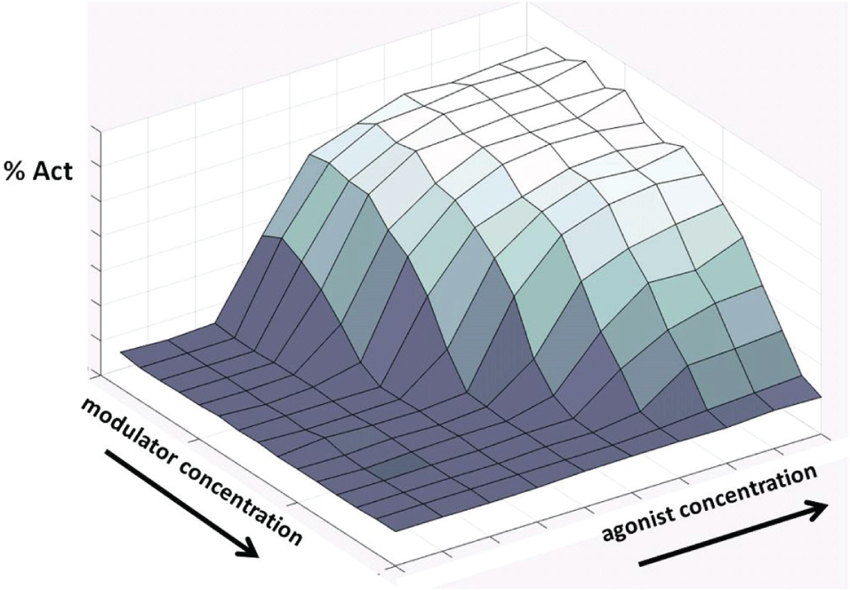
Typical negative allosteric modulator response surface in 3D. The response surface is the result of a matrix or dual titration varying agonist and modulator concentrations. The surface is then modeled as a group of curves with globally shared parameters and constraints, hence the name, global curve fit.

PLP Driving GraphPad

PLP programming support for allosteric pharmacology screening began with a simple tool to assist scientists creating the matrix of percentage activities for simple cut-and-paste input to GraphPad Prism. Initially, the key association of agonist dilution curves with specific compound concentrations was done by manually adding concentration values to a column of curve comments. These comments were then parsed by PLP to create the compound–agonist matrix for hand pasting into GraphPad Prism. As the drug program evolved and the demand for compound testing increased, more automation of the process was required.

One part of providing greater automation was bringing the step of assigning specific compounds to specific wells into ActivityBase and its XE interface. ¹² Activity Base is a screening data management system and holds fully descriptive database records of assay plates that it can associate with raw data files in a test set. For each screening run, a test set is created in XE that marries compound identity and concentration, agonist concentration assignments, and well activities. A file export of that test set is the input data file for downstream PLP analysis and model fitting.

The second part of the allosterism solution was to directly automate the GraphPad Prism analysis already in use for global curve fitting, instead of transferring the analysis over to another modeling system, such as the R statistical package, which is also supported by PLP. Allosterism is a sufficiently new target for drug discovery lead optimization that the tools and methods are being developed alongside the actual lead optimization, and continuity and consistency of analysis methods are critical. In our case, that desire for consistency meant applying automation so that production analyses could use the same GraphPad Prism analysis that was used in early development.

Bringing GraphPad Prism or Prism under PLP control meant that one script would perform data formatting, global curve fitting, and postprocessing of the fit results in preparation for downstream visualization and upload to the corporate database. The basic steps of the analysis are (1) associate compounds, concentrations, and data; (2) create and run GraphPad Prism script, and parse script results; and (3) assemble results with input data to create a visualization file. Normally, PLP executes on a server: PLP protocols are stored on the server, and results are written there or to a networked drive accessible to the PLP server. For our work, we wanted to implement the exact Prism analysis that was defined and in use by the lead identification team but automate it using PLP. To do this, we had to run Prism on the client machine while the balance of processing was on the server. Two key pieces in this were the “Run Program (on Client)” component in PLP and the built-in scripting capability in Prism itself; together, they allowed us to create a piece of automation that removed all the cut-and-paste from our process.

Instead of a fixed Prism script, we actually used PLP to build the text of the Prism script, which PLP in turn called. For one drug program, different organism-receptor pairs are analyzed together, and each organism-receptor pair is characterized by a predetermined KA or agonist dissociation constant. The varying KA values were passed to Prism by programmatically writing the values into the Prism script for each organism-receptor pair. In addition to writing the Prism script, PLP creates individual compound files each containing a matrix defining the range of agonist and modulator concentrations and the measured activity for each combination. Once started, the Prism script loops through the compound files with a simple syntax, for example, ForEach cmpd*.txt . . . Next . Pipeline needs to wait for Prism to write results files before it can extract the results. To achieve this, a Pipeline custom manipulator component enters a While loop and waits for Prism to write a “done” file indicating completion of the fitting process. See Figure 3 .

Figure 3.

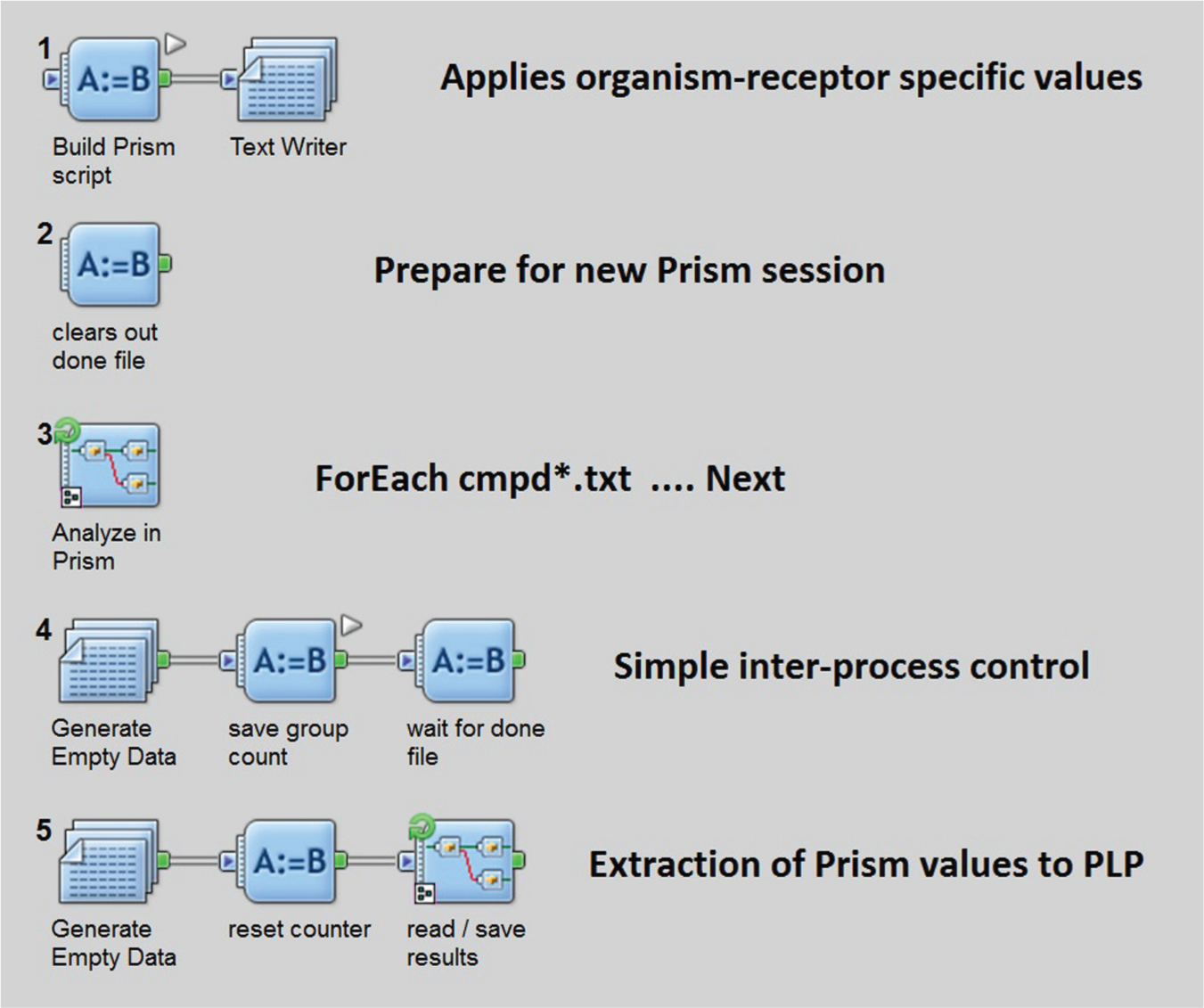
Controlling Prism from Pipeline Pilot. The basic steps of the data analysis are (1) associate compounds, concentrations, and data; (2) create and run GraphPad Prism script, and parse script results (shown); and (3) assemble results with input data to create a visualization file. This figure shows the Pipeline Pilot graphical interface for the second step of the overall process.

Multiple Fitting and Decision Tree Selection

Each of the fit parameters of allosterism can be constrained differently, depending on the drug target and specific organism–receptor pair. Not all compounds fit the same for a given target. Some compounds fit with only one set of constraints, and some fit with only different settings. Typically, we have a preferred, less constrained fit and a secondary, more constrained fit. In the case of one drug program, the preferred fit condition is successful for the large majority of compounds, and the second fit constraint, acting as a rescue fit, is used for the minority of compounds that cannot be fit with the standard constraints. For a second program, the preferred condition is the less common one, and the secondary condition is the default. In this case, the first fit captures a specific, desirable behavior not common to most compounds. Use of that preferred fit setting universally did not result in well-determined fitting across all compounds.

To address these subpopulations of compounds, we use PLP to fit each compound–response matrix twice and then select the better of the two fits using a three-step decision tree. Before any decisions, each fit is automatically reviewed and marked: it is marked as “questionable” if the standard error of a fit parameter is greater than or equal to the absolute value of that fit value. For example, if the standard error of alpha is 100 and the fitted alpha is 90, we consider alpha “questionable” and set FIT_WARN=“?”. This fit warning is used downstream in fit selection and also displayed in Spotfire. A fit can also be marked as “tilde” if Prism cannot determine a fit at all. Those two markings are the main drivers of the decision tree. In the case of a tie, when both fits are questionable but neither is undetermined, the relative size of the standard errors of each is used to automatically select the reported fit. See the details of the decision tree in Figure 4 . The selected fit is then used to annotate the original data for subsequent visualization, curve drawing, and upload to the corporate data base.

Figure 4.

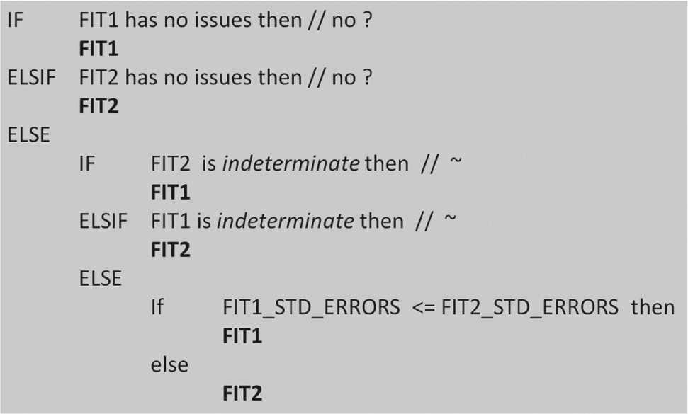
Fit selection decision tree. A simple decision tree automatically selects which fit is the best one to visualize and report to the corporate database.

Spotfire Visualization for Allosterism

Spotfire was the visualization tool used to represent allosteric assay response and also display the global curve fit determined in Prism. Figure 2 illustrates a 3D view of an allosteric response surface. However, for general usage, we create multicurve views that are projections of the 3D view to the percentage activity–agonist concentration plane. The curves on this projected view are the contour lines of the fitted response at fixed compound concentration and varying agonist concentration. Spotfire automatically generates smooth curves without an explicit plotting operation but can do that in only one dimension. Figure 5 explains how auxiliary calculated columns in Spotfire can reduce the function of the two variables, agonist and modulator concentration, effectively to multiple functions of one variable, one for each contour line, which can be plotted automatically by Spotfire. An additional tab in our allosteric Spotfire template allows viewing of the results in the activity versus compound concentration plane. Here, the user performs a dynamic query by selecting a slice of the response surface to “look into the page” and expose the receptor response at fixed agonist concentration and varying compound concentration. See Figure 6 .

Figure 5.

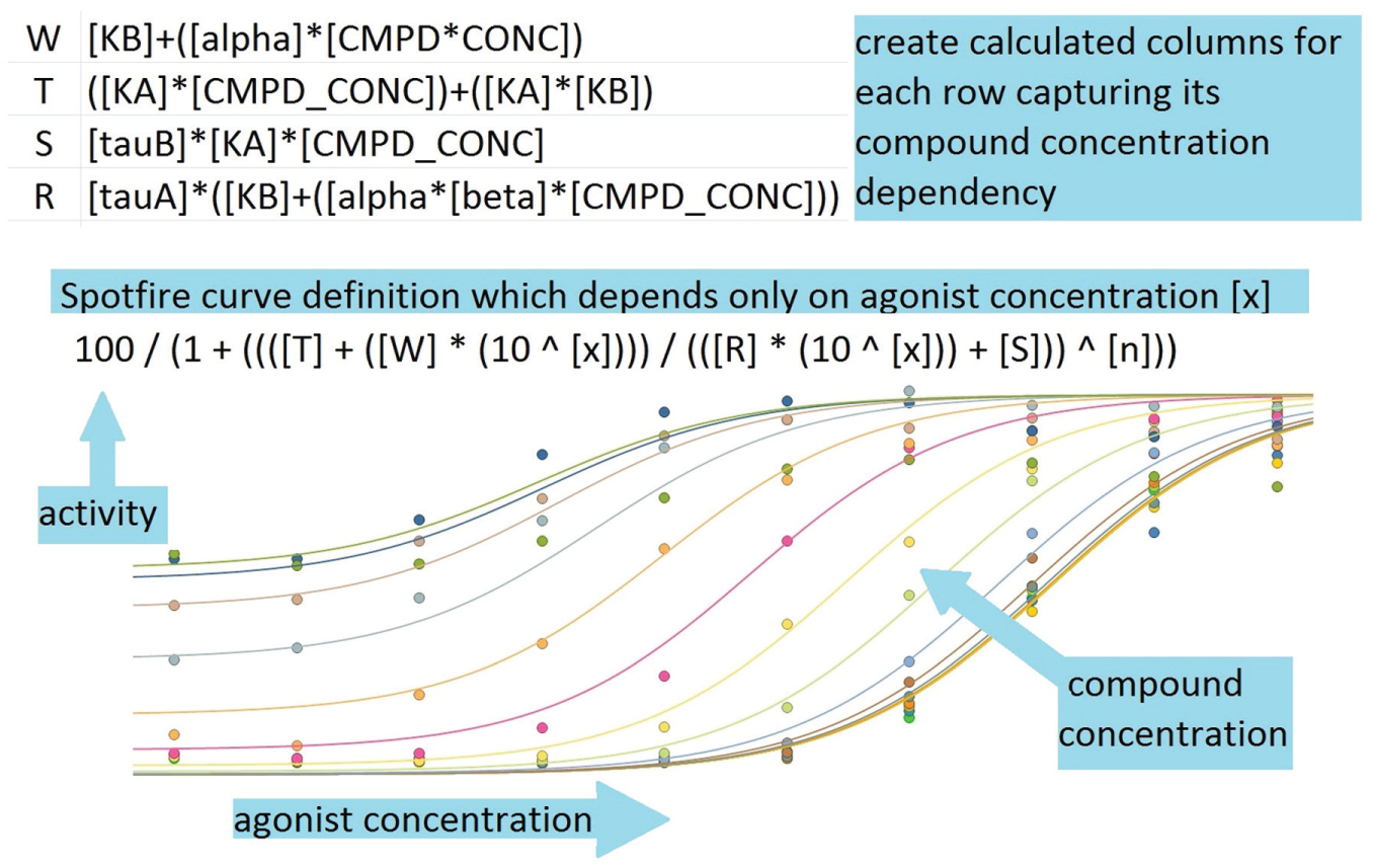
Drawing allosterism curves in Spotfire. Auxiliary columns are created to enable automatic drawing of the allosterism function of two concentration variables.

Figure 6.

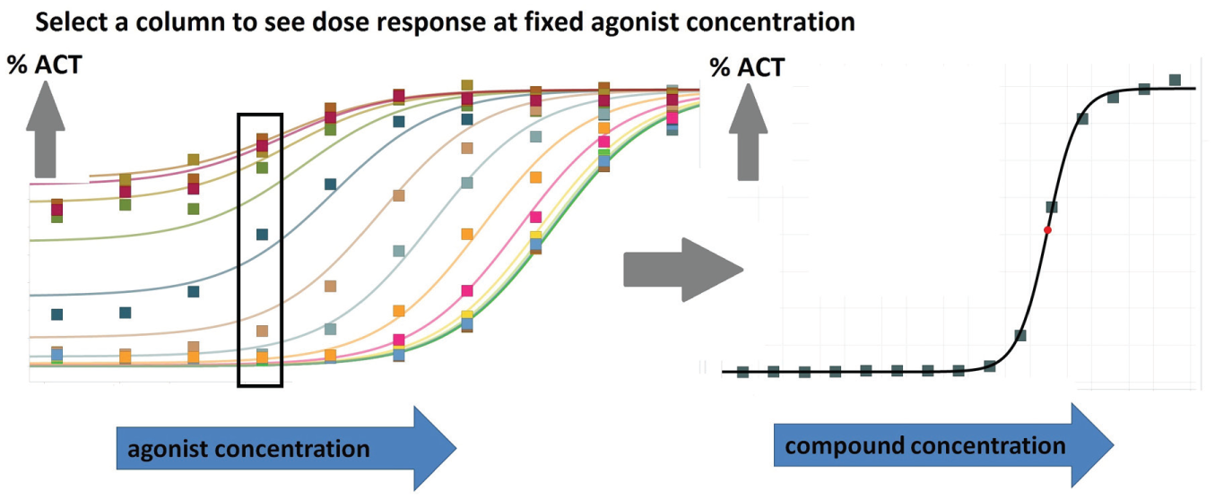
Taking a slice of a response surface. The user “rubberbands” a slice of the response surface to “look into the page” and expose the receptor response at fixed agonist concentration and varying compound concentration.

Case 2: Coagulation Analysis

Background

The second case considers our work on developing data automation to support coagulation experiments. Research in the pharmacology of coagulation can require the use of clinical instrumentation with sample and data handling far afield from 384-well plates and plate readers often used in pharmaceutical in vitro pharmacology. ¹³ For our coagulation studies, the laboratory instrument is the STA-R Evolution Plus from Diagnostica Stago, which features a VDS Mechanical Clot Detection System (viscosity-based detection system). The Stago monitors the movement of a ball bearing between two magnets and records the clot time as the time it takes for the ball bearing motion to stop due to clot formation. ¹⁴

The STA-R Evolution is an example of a higher-throughput coagulation analyzer that can use vacutainers or Eppendorf tubes, is widely used in clinical settings, and has the ability to use small sample volumes. Although built for high throughput in a hospital setting, supporting this kind of instrument in a lead optimization laboratory presents data automation challenges that required us to employ the methods first developed for allosterism and global fit. For coagulation assays, the sample handling (as opposed to the modeling, which is a simple interpolation), precluded using standard plate-based analysis tools, such as ActivityBase XE.

The challenge here was to accept the data and compound assignment files directly, without ActivityBase XE; run GraphPad Prism; and report on the results, automatically. Prior to automation, approximately 8 h was being spent purely on data analysis: managing Excel, populating Prism, and creating reports in Microsoft PowerPoint. The goal of the automation was to eliminate cut and paste at each step: data loading, Prism analysis, and reporting. At the same time, a degree of flexibility was required to allow individual sample result replacement, which can be required for coagulation assays.

The result was two PLP scripts working with a Spotfire template. Processing time was reduced from about 8 h of cut and paste to approximately 1 h. The first script accepts raw data and compound delivery sheets and creates a Spotfire-compatible file and an Excel summary report for inclusion in a reporting email. The second PLP script uses the output of the first to create a file formatted for upload to the corporate database. Cut and paste was eliminated, and flexible Spotfire reporting replaced fixed images in Powerpoint.

PLP enables the use of hash tables for saving in-process data using the association between string “keys” and data values. A hash table is a general purpose data structure, basically an in-memory key-value database for storing intermediate values or results. ¹⁵ In the context of PLP’s row-by-row processing, this data structure is very useful for across-row calculations or associations. The Stago PLP script saves to and retrieves from hash tables to calculate ratios across species and across activity and liability tests. This extra step while the data are in hand avoids an auxiliary postprocessing step, which is often required when comparing panel results. These ratios, though not uploaded to the corporate database, are displayed in Spotfire for review by the project team.

Case 3: GPCA for Enzyme Kinetics Modeling

Background

The third case considers the automation of global curve fitting for enzyme kinetics modeling. “Kinetic profiling of a drug binding to its target can be used to reveal important mechanistic parameters including drug-target residence time.”^16(p59) GPCA for kinetic profiling of enzymatic targets “does not require specialized instrumentation of label-free methods such as surface plasmon resonance. It can be conveniently performed in an ordinary biochemistry lab.”^16(p62) Figure 7 illustrates the results of an experiment measuring enzyme product creation over time for 11 compound concentrations. GPCA achieves a great deal in one experiment, but it relies heavily on global curve fitting as implemented in Prism. The data loading, constraint adjustment, and reporting from Prism can become onerous when extended to larger data sets, such as 32 compounds run against three enzymes. Prior to the introduction of automation, an analysis of a three-plate experiment with 96 manually adjusted fits could take a scientist approximately 3 d to complete. Automation means that the entire process, much of which is unattended, takes about 2 h.

Figure 7.

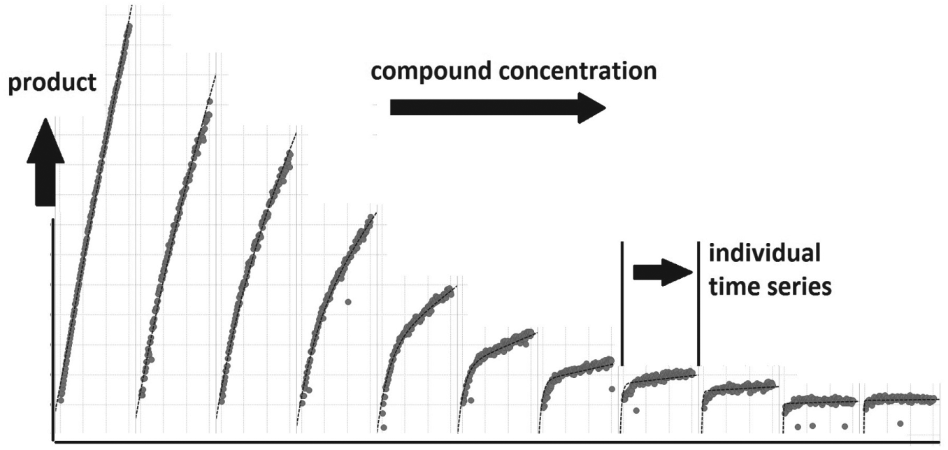
Trellis view of global progress curves. Each of the panels of the “trellised” figure is a time course of enzyme product creation for 1 of the 11 compound concentrations tested.

We initially looked at GPCA in the context of global curve fitting for allosterism, but we did not consider it amenable to automation because each compound required custom fitting in what seemed to be a wide-ranging trial-and-error process. Further review of the manual process for GPCA exposed an underlying iterative process that could be simplified to stepping through three sets of Ki settings. Fit 1: Ki shared and >0, with an initial value of 1000. Fit 2: Ki shared and >0, with an initial value of 0.10. Fit 3: Ki fixed and =0.01 for all curves. The fits are performed in order, starting with the highest Ki, and the first one that successfully fits ends the process for that compound–enzyme combination.

One of our main concerns in creating a fully automated solution was the possibility that some compound curve sets would not fit at all and any manual results would be difficult to include with the results of automation. To address this at the outset, a new intermediate stopping point was created for the analysis as compared with the allosteric solution. The process is split in two pieces: create and compile. Between the scripts, there is a point for manual adjustment of data exclusion and fit constraints.

Initially, the script Create is run: all of the fitting is attempted, and individual Prism files are created containing the best effort of the automation for each compound–enzyme combination. At this point, the scientist can review and validate the results in Spotfire and see what has fit, what has not, and if a threshold is required for automated data exclusion. A typical threshold excludes any values above the point at which the DMSO-only curve begins to show curvature. If a threshold is required, Create is rerun with this threshold in place, and the results are rechecked in Spotfire.

The successive fit procedure in Create operates by examining each results file for any indeterminate fit parameters, indicated by a tilde or ~. Fit 1 is run, and then all of the fit results are reviewed for tilde, and the results are stored in a hash table for later annotation. Any compound–enzyme data sets that are tilde for Fit 1 are rerun with Fit 2 and similarly with Fit 3. As it finishes, Create writes a log file of what Prism files were created and when they were written.

If a compound set is not successfully fit in Create, its individual Prism file can be manually opened in Graphpad Prism, the constraints or initial values modified, manual data exclusion performed as required, and the file saved. Compile reads the Create log file and builds a list of manually adjusted files: the files that have been modified since the automated Create step. If a Prism file is altered from its original automated analysis state, Compile opens it in Prism so that it executes as-is and exports a results file. This fresh results file is parsed, and its fit values replace the original results in an updated Spotfire-ready output file. At the end of the process, Spotfire represents the state of the Prism files as they were left, including automatically generated as well as manually adjusted fitting results. Any fits that were manually adjusted are noted as such in Spotfire. At any time, a Prism file can be reopened, adjusted, and then Compile rerun to update the Spotfire file. For our work to date, we have had 100% fitting with the three-fit alternative, and the manual step has been used simply for data exclusion. For future work, if an additional fit or constraint setting is required, it can easily be added to the cascade of fits.

Discussion

In these case studies, scientist requests, expressed in close and interactive collaboration, were the drivers in evolving and refining the automation tools to bring them to full utility. One key to success was matching that collaboration with a graphical data flow programming environment with a wide range of application-specific components, which enables a high degree of code reuse so that new or updated methods can be delivered within days, rather than weeks. A second key to success was maintaining continuity and consistency of analysis methods by directing the automating of GraphPad Prism and skipping the step of cross-validating the results of two different modeling systems. We have reviewed three scenarios demonstrating how data flow programming can automate special analysis requirements while working alongside visualization tools to address the ever-increasing demands on scientists for data analysis and interpretation.