Sage Journals: Discover world-class research

Abstract

The AstraZeneca Compound Management group uses high-performance liquid chromatography–mass spectrometry for structure elucidation and purity determination of the AstraZeneca compound collection. These activities are conducted in a high-throughput environment where the rate-limiting step is the review and interpretation of analytical results, which is time-consuming and experience dependent. Despite the development of a semiautomated review system, manual interpretation of results remains a bottleneck. Data-mining techniques were applied to archived data to further automate the review process. Various classification models were evaluated using WEKA and Pipeline Pilot (Pipeline Pilot version 8.5.0.200, BIOVIA, San Diego, CA). Results were assessed using criteria including precision, recall, and receiver operating characteristic area. Each model was evaluated as a cost-insensitive classifier and again using MetaCost to apply cost sensitivity. Pruning and variable importance were also investigated. A 10-tree random forest generated with Pipeline Pilot reduced the number of analyses requiring manual review to 36.4% using a threshold of 90% confidence in predictions. This represents a 45% reduction in manual reviews compared with the previous system, delivering an annual savings of $45,000 or an increase in capacity from 25,000 analyses per month up to 45,000 with the same resource levels.

Keywords

LC-MS data mining random forests WEKA Pipeline Pilot

Introduction

As the size of compound collections has increased, so too has the need for rapid analytical methods of quality assurance. A number of techniques have been developed to achieve this, including (but not limited to) liquid chromatography (LC) and mass spectrometry (MS),¹ nuclear magnetic resonance,² and charged aerosol detection (CAD).³ A common requirement for many of these methods is that they can be integrated into workflows characterized by automated systems capable of high throughputs. As instrumentation has become more sophisticated with the introduction of automated compound storage⁴ and nanoliter dispensing,⁵ so too have the demands on data handling and interpretation.⁴ An effective instrument data management system to process, store, and organize the volume of data produced is essential,⁶ and meeting the high-throughput demands may be achievable only using software-supported spectra interpretation.⁷

The overall quality of AstraZeneca’s corporate compound collection is monitored by Compound Management (CM). The purity and structural identity of compounds entering the collection are established using reversed-phase high-performance chromatography coupled with MS with an additional CAD to measure concentration,⁸ hereafter referred to as the LC-MS system. In addition, LC-MS activities are required to support the formation of screening collections for high-throughput screening (HTS) campaigns as well as the provision of “just in time” analysis to support later-stage screening projects.

To meet the challenges of this high-throughput environment, the CM group developed an LC-MS platform capable of automatically passing analyses in which a set of thresholds were detected in the preprocessed data generated by the instrumentation. As a result, 33.8% of the analyses performed were automatically flagged as “passed,” with the remaining analyses reviewed by domain experts.⁸ Despite the success of the autopass functionality, the interpretation of analytical data remains the bottleneck in the LC-MS workflow. The available archive of more than 700,000 analyses, many of which were annotated by LC-MS experts, was identified as an opportunity to apply a data-mining approach to further automate the classification of LC-MS results.

Applications of data-mining algorithms are increasingly prevalent in pharmaceutical research and health care more widely. Structure-activity relationships, hit identifications, and disease diagnosis can all be facilitated by decision tree (DT) induction.^9,10 The basic process involves recursive partitioning of data into more homogenous subsets by passing each record through a series of if-then rules arranged in a tree structure.

Particular focus has been given to ensemble learning models, which involve using a number of classification models in combination. These techniques are less prone to problems associated with overfitting as the resulting models are collectively less biased toward a particular training data set. Wu et al.¹¹ evaluated ensemble techniques with the aim of diagnosing ovarian cancer based on peptide/protein intensities. Random forests (RFs) outperformed all other methods in the study, which also raised the issues of data preprocessing, noise reduction, and variable selection as additional challenges faced when making diagnoses using MS data. Burbidge et al.¹² applied a support vector machine (SVM) to structure-activity relationship data and concluded that SVM was an “automated and efficient deterministic learning algorithm” capable of highly accurate classification (error rate of 0.1269).

That the application of classification models to LC-MS results in the “-omics” cascade (genomics, transcriptomics, proteomics, and metabolomics) is well documented,^13-15 but no examples were found of the use of these techniques for quality assurance of small-molecule compound libraries. A number of features described herein are, to my knowledge, novel, such as the classification of each individual integrated peak and the application of an overall confidence per analysis.

Methods

A number of data-mining techniques were applied to data from the existing LC-MS database in order to construct classification models capable of predicting the pass/fail outcome of an LC-MS analysis. The WEKA¹⁶ software suite was used to build, test, and evaluate a diverse set of models, including DTs, SVMs, neural nets, and various ensemble techniques such as RFs and alternating decision trees (ADTree). The Analysis and Statistics Library in Pipeline Pilot was also used to evaluate an RF implementation owing to the ability to output a confidence measure against each prediction. Various pruning techniques were also evaluated whereby the complexity of a model is minimized with little or no reduction in performance. Cost-sensitive classification was investigated using MetaCost.¹⁷

The general pattern of the analytical data stored in the existing LC-MS database was represented by a tuple for the analysis containing information on the target compound, the expected mass, chromatographic results, and source vessel. Additional tuples were created for each integrated peak from the UV chromatogram, with information on the percentage purity by UV and the percentage spectral purity by MS for two ionization methods (electrospray ionization [ESI] and atmospheric pressure chemical ionization [APCI]).

The data were denormalized from the hierarchical structure into records representing each integrated peak. The classification models instead used a pass/fail class label for each peak, which could ultimately be aggregated back to the analysis level to determine the overall outcome of an analysis event.

A process of data cleaning was performed to remove any invalid or erroneous values from the data set. A total of 2,443 analyses, containing a total of 10,650 integrated peaks, were marked by users as instrument errors during manual review. These records represented 0.46% of the total data available. They were filtered out from all experimental data sets as the data produced was spurious and may have polluted the construction of classification models if included. Different LC-MS instrumentation used by CM recorded ultraviolet (UV) peak height, UV peak width, CAD peak height, and CAD peak area using different units. A multiplier was used to normalize these values across the different instruments.

Data in the LC-MS database were generated by analytical instrumentation with subtly different configurations. All MS detectors used ESI, but some instruments also included an APCI system. These missing values were assigned the value of 0. This had little effect on the data overall, as the spectral purity by MS values for individual ionization techniques and ion modes was not considered directly. Instead, a function was used to find the maximum spectral purity value across each ionization method and ion mode. This function is described below. The likelihood of a sample being detected may have been slightly less if processed on an instrument with only ESI ionization, but this was not considered significant.

Null values for MS spectral purity or percentage purity by UV were considered valid results indicating that the target mass or any of the adducts included in the search pattern had not been detected. As such, null values were also assigned a zero value. A full list of the fields recorded for each peak is included in Supplementary Table S4.

Additional derived attributes were calculated for each peak. These were the outcome of consultations with LC-MS domain experts and were considered potentially useful when classifying analyses as pass or fail. The attribute get_closest_peak was included to help identify a particular type of issue. The LC-MS instruments perform the task of identifying each eluted peak when processing raw data. Although this is generally successful, sometimes a slight aberration or “shoulder” during chromatography can cause the instrument to incorrectly divide a single peak into two. This effect is described in the simplified representation of a chromatogram in Figure 1 . 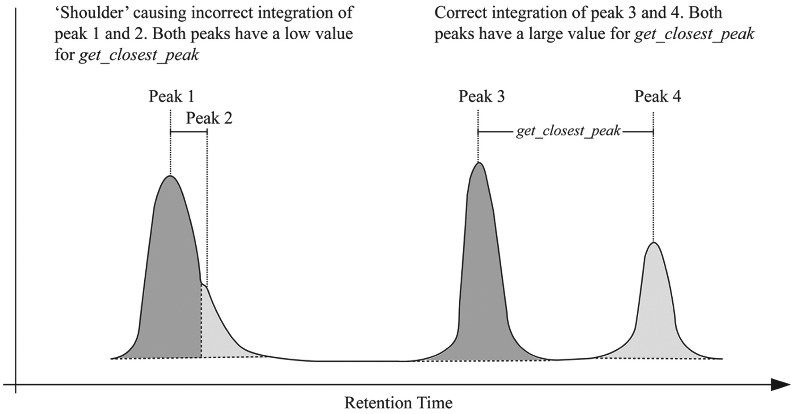A further example from an actual analysis is included in Supplementary Figure S5. The get_closest_peak attribute measures the distance in retention time from each peak to the closest peak, eluted either before or after in the chromatogram, and was used to try to identify these types of integration problems. The remaining derived attributes were as follows; num_of_peaks, the total number of peaks eluted in the DAD chromatogram for the given sample; get_cad_percent, the area under the CAD chromatogram for a given peak, expressed as a percentage of the total area; and horz_max_ms_purity, the maximum spectral purity for a given peak from the one or two ionization techniques employed by the MS detector. Each has two ion modes, giving a total of either two or four values.

Figure 1.

Detection of peak integration errors using the get_closest_peak attribute. A small value could potentially help to identify single peaks incorrectly integrated as two peaks.

Training/test data sets (2/3 training and 1/3 test data) of increasing sizes were created. Initial evaluations were performed with subsets of the available data due to processing times and hardware constraints, with the full data set used for later-stage analysis. Although this study ultimately used a binary classification label of pass or fail, different types of pass/fail results were identified. A process of stratification was applied to the data sets to ensure that the proportions of these types of outcomes were maintained and reflected the distribution found in the data set as a whole. This was done to avoid any bias toward a particular outcome.

The class attributes provided increasing levels of detail regarding the pass/fail outcome for each peak and how that outcome was reached. The first class label (class label 1) was a binary classifier with possible outcomes of pass or fail. The second (class label 2) split these two categories into a more detailed class label, with possible values of auto pass, agreed pass, overwritten pass, agreed fail, and overwritten fail. The third class label (class label 3) divided the values of the second level into even more detailed outcomes, such as ms fail uv fail overwritten pass or ms pass uv fail agreed fail. All possible outcomes for each peak are included in Supplementary Table S5. A diagram and description of the manual review process are provided in an earlier article.⁸

Cross-validation was used for the initial assessment of learning algorithms and for the experiments on pruning methods. Smaller training sets are more likely to be biased by particular features of the data and therefore suffer from overfitting. Standard 10-fold cross-validation was used, in which data are divided randomly into 10 folds or partitions. One of the folds is used as a holdout test set with the remaining nine used as training data. The process is repeated with each of the 10 folds used as the holdout test set. Finally, an average error estimate is calculated from all 10 results.

When larger data sets were used to assess model performance, cross-validation became less essential and more computationally expensive. The amount of data used for the later assessment of classification models and for the experiments on cost sensitivity contained approximately 500,000 instances. Because of memory constraints, cross-validation was not applied as maximizing the size of data sets was preferred to emulating a large data set by applying cross-validation.

A number of measures were considered to quantify various aspects of performance. LC-MS data in this domain are a binary decision of pass or fail with regard to structural identification and purity. As such, there are four possible outcomes for each analysis: true positive (TP), an actual pass that was correctly predicted as a pass; true negative (TN), an actual fail that was correctly predicted as a fail; false positive (FP), an actual fail that was predicted as a pass; and false negative (FN), an actual pass that was predicted as a fail.

The overall accuracy and error rate for predicted outcomes on test data were used as simple measures of the performance of learning models. Accuracy is the number of correct classifications divided by the total number of classifications shown in eq 1:

a c c u r a c y = \frac{T P + T N}{T P + T N + F P + F N}

Conversely, error rate is calculated as in eq 2:

e r r o r r a t e = 1 - a c c u r a c y

The kappa statistic, a measure of overall success rate that also takes into account how many correct classifications would be expected from a random classifier, was recorded for each classification model. So too was the recall, precision, and F-measure, all of which examine the overall accuracy taking into account the different classification errors.

Recall expresses the number of TPs as a percentage of the total number of positives, shown in eq 3:

r e c a l l = \frac{T P}{T P + F N}

Precision calculates how often a prediction of pass is correct by comparing the number of TPs with the total predicted to be passes, shown in eq 4:

p r e c i s i o n = \frac{T P}{T P + F P}

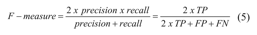
F-measure combines recall and precision into a single value, shown in eq 5:

F - m e a s u r e = \frac{2 x p r e c i s i o n x r e c a l l}{p r e c i s i o n + r e c a l l} = \frac{2 x T P}{2 x T P + F P + F N}

As the true positive rate (TPR) of a classification model increases a cost is incurred in terms of the false positive rate (FPR). The optimum situation is one in which an increase in TPR can be achieved with minimal increase in FPR. The relationship between these two rates can be visualized using receiver operating characteristic (ROC) curves, and the area under the ROC curve (AUC) describes the quality of the classifier, with a larger AUC signaling a better performance.

Different costs for misclassifications can be defined by a cost matrix C(i,j), where i is the actual class and j is the predicted class.¹⁸

C (i, j) = (\begin{matrix} 0 & 1 \\ 1 & 0 \end{matrix})

C (i, j) = (\begin{matrix} - 1 & 20 \\ 0.5 & 0 \end{matrix})

Eq 6 represents a cost matrix that assumes the same cost for FP and FN misclassifications. Eq 7 defines a cost matrix that assigns a much higher cost to FN misclassifications than to FP and rewards TP more than TN by assigning a negative score.

Such cost matrices can be applied to the predictions of a classifier, with the effect of altering the assessment of performance according to the differing costs of misclassifications. A more powerful approach is to make the classifier cost sensitive by incorporating the cost matrix during the construction of the classification model. The predictions themselves are altered rather than the evaluation of the predictions according to costs. This was achieved using the MetaCost meta-learner.¹⁷ MetaCost is not an algorithm for building classification models but a “wrapper” used in conjunction with an arbitrary base classifier to make the underlying classification algorithm consider a cost matrix during its construction. MetaCost does not make any changes to the base classifier, treating it like a black box. It was therefore possible to apply MetaCost to a range of different classification algorithms.

Pruning

DTs often contain a structure that accommodates anomalies or outliers in the training data. For DTs to perform more accurately on test data or unseen future data, a process of pruning is required. This produces a more generalized form of the tree, avoiding problems of overfitting. Both prepruning and postpruning methods were evaluated. Prepruning involves the decision not to continue dividing subsets of the training data during the construction of the tree. Postpruning involves removing subtrees from the overall DT after the full tree has been constructed.

In a fully unpruned DT, splitting ceases when the data produced from a node is 100% pure with regard to the class label or when a split produces a single instance. By applying a minimum number of instances per leaf node, further splitting will not be applied even if the purity of the data partitioned is less than 100%. This eliminates the lower branches of the DT and produces smaller, more generalized models. The methods of assessing which attributes to split on, such as information gain¹⁹ and Gini index,²⁰ can be used to test for a threshold below which further splitting will not occur. This represents a tradeoff, as too high a threshold will result in oversimplified trees that perform poorly and too low a threshold will provide insufficient simplification to avoid overfitting.

Other pruning methods investigated were reduced-error pruning²¹ (postpruning) in which some of the training data are used specifically for pruning, and SimpleCart DT, the cost-complexity algorithm used in classification and regression trees.²² This method considers both the error rate (the number of tuples misclassified) and the complexity of the subtree in terms of the number of leaf nodes.

Classification models were examined in terms of number of nodes/leaves and variance in complexity, comparing unpruned models with prepruning and postpruning techniques. A data set containing approximately 100,000 records was used to build DTs. Ten-fold cross-validation was applied in each case to produce sets of 10 DTs. The average, standard deviation, and variance of both the number of leaf nodes and the total number of nodes in the trees were recorded. Measurements of accuracy, precision, recall, ROC area, kappa statistics, and FP/FN rates were considered to evaluate the performance of each algorithm and pruning method. These performance measures were calculated by combining the results of all 10 models in each set.

Ensemble Methods of Classification

A number of ensemble methods were evaluated in which classification models are combined so that the overall classification decision is the amalgamation, by an average or weighted average, of the decision outcomes of each model. This is analogous to decision-making “by committee.” These methods can often greatly increase the accuracy of classification and are less prone to overfitting because the combined decision avoids any bias that may be caused by the idiosyncrasies of one particular set of training data.²³

There are a number of methods of combining models such as bagging,²⁴ boosting,²⁵ RFs,²⁶ and stacking.²⁷ In all cases, the main advantage is one of variance reduction; the combined outcome of diverse classifiers compensates for the error rate of any individual classifier.²³ A disadvantage with some but not all ensemble methods is the loss of interpretability, as the base classifiers cannot be visualized in the same way as an individual classifier such as a DT.

RFs possess a number of advantages over other ensemble techniques and have been widely applied in the field of life sciences, particularly -omics data, in which the number of attributes can often be vast.²⁸ RFs combine two methods to build classification models, namely, bagging and random feature selection. As such, they introduce randomness in two, possibly complementary areas. Sampling with replacement is conducted as with standard bagging, producing bootstrap samples for training that contain n number of instances randomly drawn with replacement from the learning set of n instances.²⁹ A random set of attributes is then generated and the base model is constructed using only those attributes. The Gini index is used as the splitting attribute selection mechanism. Some of the advantages of RF algorithms are that they are relatively robust to outliers and noise, they are faster than bagging or boosting, and they can provide useful internal estimates of error, strength, correlation, and variable importance.²⁶

Results

Evaluation of Classification Models

In accordance with a simplicity-first approach to data mining, learning models of increasing complexity were evaluated, beginning with simple classification rules and progressing through more complex algorithms. A data set of approximately 500,000 records was used to construct each of the models listed in Table 1 , with the exception of the RFs generated with Pipeline Pilot, in which all available data were included (773,176 peaks) because of lower memory requirements for this platform.

Table 1.

Performance of Classification Models.

Model	Accuracy (%)	Precision	Recall	F-Measure	ROC Area	Kappa	FP Rate	FN Rate
ZeroOne	85.95	0.739	0.86	0.795	0.5	0	0	1
DecisionStump	94.84	0.949	0.948	0.949	0.902	0.7899	0.033	0.164
SMO	96	0.96	0.96	0.96	0.913	0.8331	0.022	0.152
FT	97.43	0.974	0.974	0.974	0.954	0.891	0.01	0.121
NaiveBayes	93.28	0.947	0.933	0.937	0.977	0.7572	0.068	0.064
REPTree	97.27	0.972	0.973	0.972	0.978	0.8831	0.009	0.139
J48	97.38	0.973	0.974	0.973	0.979	0.8883	0.009	0.128
J48 (Bagging)	97.44	0.974	0.974	0.974	0.981	0.8908	0.009	0.128
SimpleCART	97.86	0.979	0.979	0.979	0.986	0.9102	0.007	0.105
ADTree	97.10	0.971	0.971	0.971	0.991	0.8762	0.011	0.14
Multilayer	97.31	0.973	0.973	0.973	0.991	0.8859	0.011	0.124
NBTree	97.60	0.976	0.976	0.976	0.994	0.8988	0.01	0.108
LMT	97.84	0.978	0.978	0.978	0.994	0.9084	0.008	0.103
RF (5trees)	99.88	0.999	0.999	0.999	1	0.9952	0	0.005
RF (10trees)	99.97	1	1	1	1	0.999	0	0.001
RF (20trees)	99.99	1	1	1	1	0.9999	0	0
RF (50trees)	100	1	1	1	1	1	0	0
RF (5Trees) PipelinePilot	95.99	0.796	0.962	0.871	-	-	0.0347	0.0054
RF (10Trees) PipelinePilot	96.06	0.774	1	0.873	-	-	0.039	0.0054
RF (20Trees) PipelinePilot	96.07	0.775	1	0.873	-	-	0.0393	0
RF (50Trees) PipelinePilot	96.08	0.77	1	0.873	-	-	0.0392	0
RF (100Trees) PipelinePilot	96.09	0.776	1	0.874	-	-	0.0391	0

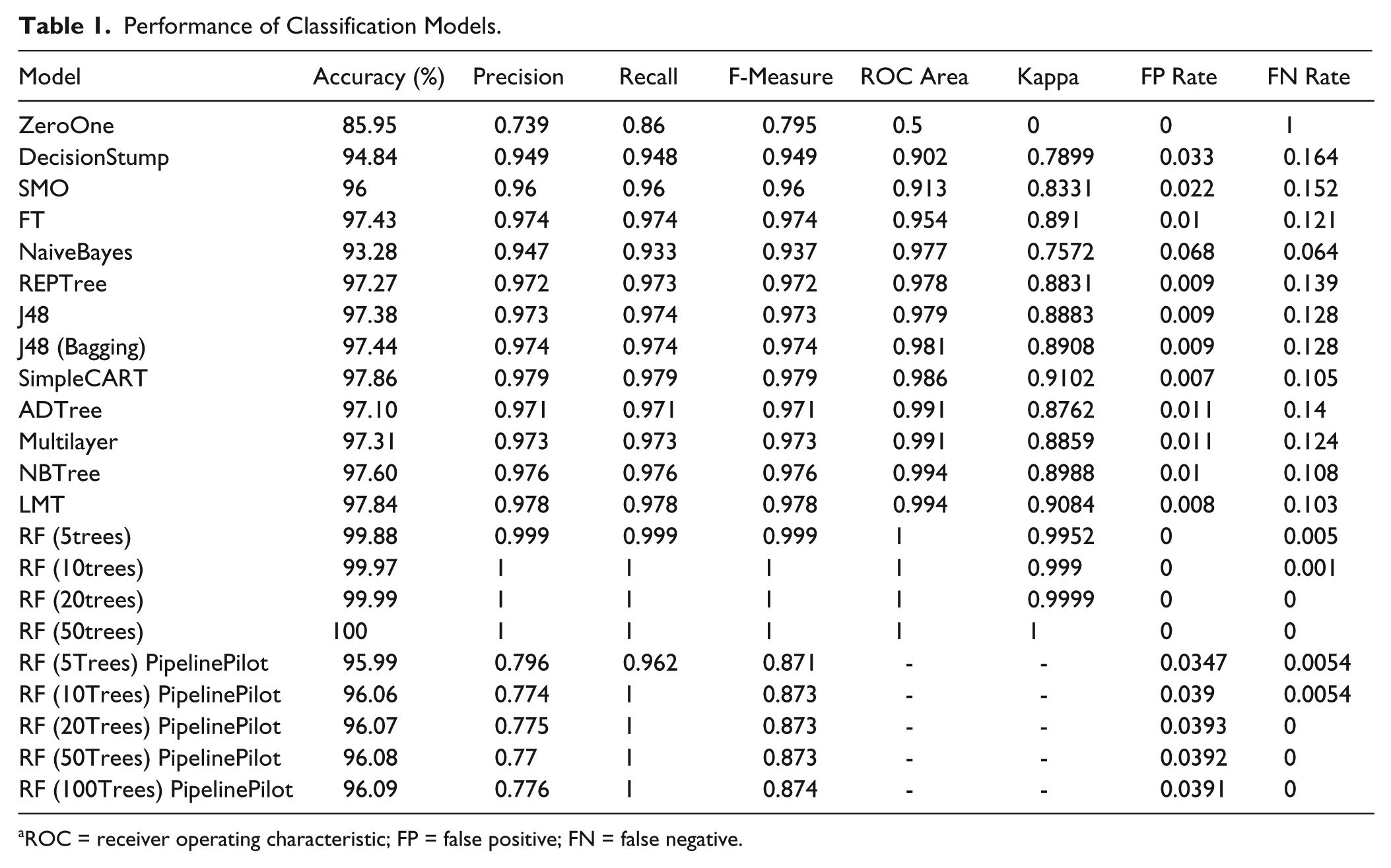
ROC = receiver operating characteristic; FP = false positive; FN = false negative.

Because the majority of integrated peaks are fails, the ZeroOne algorithm simply predicted the class of all peaks as fail and was accurate for 85.95% of instances. Clearly this rule is of no use in making predictions, reflected in a Kappa score of 0, an FPR of 0, and an FNR of 1. It is useful, however, in establishing a baseline against which the other classification models can be compared. The single test on percent purity by UV produced by the Decision Stump is successful in predicting a large number of instances, with measurements of 0.949 and 0.902 for F-measure and ROC area, respectively. This highlights the fact that as expected, the attribute percent purity by UV is the single most important variable in the decision of pass or fail. The more sophisticated algorithms all increased the predictive performance of the remaining instances, with RF showing the highest performance on all measures with an accuracy close to 100% when using 20 and 50 tree ensembles.

Further experiments were carried out using Pipeline Pilot to investigate the performance of the RF available in this software. The motivation for this was that much of the existing LC-MS system is implemented in Pipeline Pilot so the barrier to future integration with the current operational workflow would be low. Crucially, the Pipeline Pilot model was capable of outputting confidence statistics on all class predictions. This feature was particularly desirable as it allows the partitioning of results into high confidence predictions (autopass and autofail) and low confidence predictions that require manual review.

The maximum amount of available data from the legacy LC-MS database (773,176 peaks) was used to train and test the RF models in Pipeline Pilot. Forests were constructed using 5, 10, 20, 50, 100, and 200 trees in the ensemble. The results of these experiments are also shown in Table 1 . All RF models showed high performance, with the 5-tree and 10-tree models producing an FNR of 0.0054 (4151 FN results) and 0.0054 (4181 FN results), respectively. The remaining RF ensembles showed very little difference in performance when the number of trees was increased, supporting the findings of Oshiro et al.³⁰ that at some point, increasing the number of trees in an ensemble produces no significant gains in accuracy.

The RF models constructed using Pipeline Pilot were also assessed in terms of the confidence measures with which predictions of class were made. The data for all models are summarized in Figure 2 , which shows the percentage of predictions that had a confidence value in excess of 90% (represented as >0.9). A single-tree classification and regression model was included for comparison, labeled RF_TreeModel. All RF models were able to make more confident predictions of class outcomes compared with the single-tree model. The proportion of high-confidence predictions declined as the number of trees in the ensemble was increased, with the five-tree ensemble showing the highest proportion of high-confidence predictions.

Figure 2.

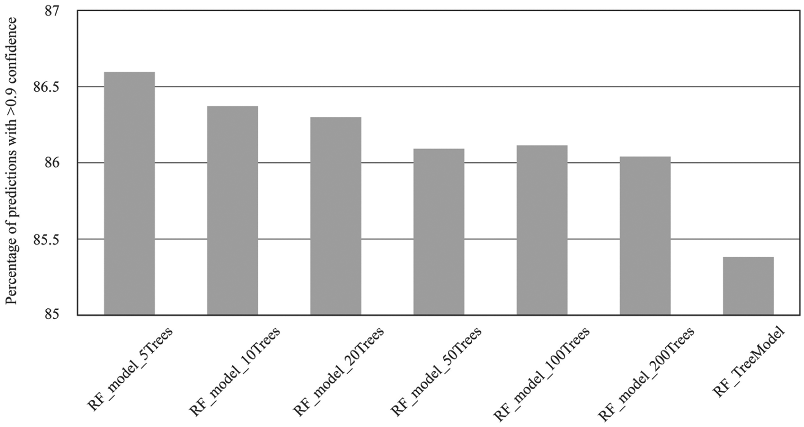
Effect of random forest tree number on the percentage of high-confidence (>0.9) predictions.

To assess the impact of a system as described above, an analysis was performed on the test data used to evaluate the RF (10 trees) in Pipeline Pilot. All 773,176 peaks were grouped into their respective samples, producing 175,893 unique analyses. Various confidence thresholds, referred to as min conf, were investigated to test the effect on the number of analyses that would require a manual review. Each group was then tested to see if any “pass” predictions were present. If found, the samples were labeled as autopass if the confidence on pass predictions was >min conf and pass-requires-review if <min conf. For samples in which all peaks were predicted as failed, the value of the prediction with the lowest confidence was tested, with >min conf labeled as autofail and those with at least one prediction where the confidence was <min conf labeled as fail-requires-review. The results are summarized in Figure 3 .

Figure 3.

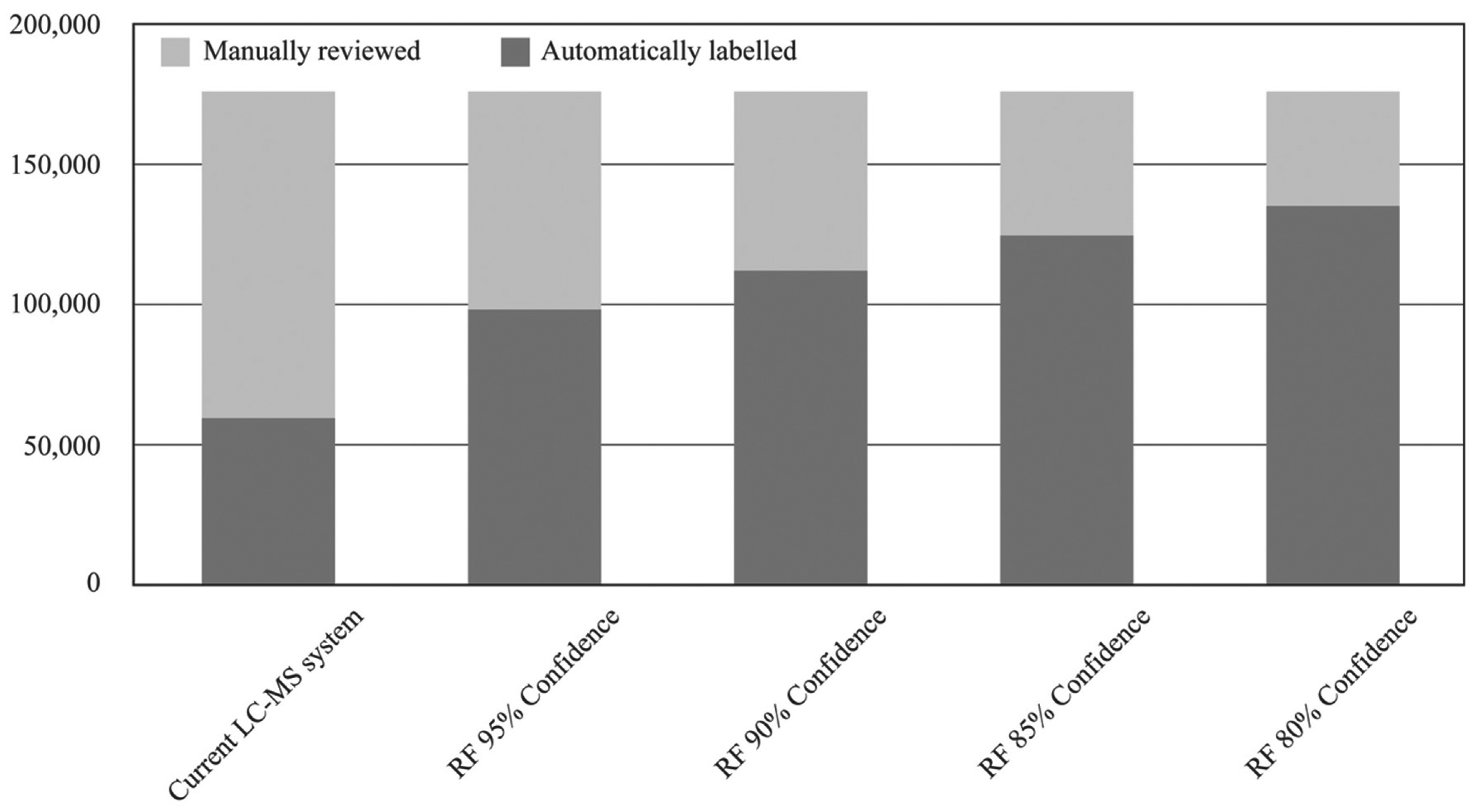
Comparison of automatic and manual reviews for the current liquid chromatography–mass spectrometry system versus the random forest approach.

For comparison, the current LC-MS system was able to automatically pass 59,497 analyses, with the remaining 116,396 (66.2%) requiring a manual review. When the RF model is applied, the number of analyses requiring a manual review drops to 77,840 (44.3%), with min conf set at 95% and 40,688 (23.2%) when min conf is relaxed to 80%. Following discussions with domain experts, a figure of 90% for min conf was considered a suitable compromise between accuracy and a reduction in the number of manual reviews. This figure could be adjusted to suit the requirements of specific LC-MS processes. When min conf was set to 90%, the number of analyses requiring manual review dropped to 64,087 (36.4%), a 45% reduction in the number of manual reviews. Within the 111,806 analyses automatically passed, there would have been 1966 (1.8%) FP results and only 335 (0.3%) FN results. Clearly this is a significant reduction in the amount of resources required in terms of reviews by expert LC-MS technicians. For the data included in this test set alone, 52,309 analyses would have been removed from the manual review process.

Cost-Sensitive Classification Using MetaCost

As with many real-world data sets, the costs of different types of misclassification in this domain are unequal. An FP result for an analysis could potentially lead to a low-quality compound being included in the screening collection. The reasons for failure could vary: the purity was recorded as lower than 85%, an impurity more sensitive to UV absorption was present, the compound could not be detected by UV, and the compound was pure but was a different structure from the one expected. For most HTS campaigns, activity in an assay is detected by a cluster of hits rather than a single reactive compound. Libraries are synthesized in which a number of compounds share a similar parent structure and occupy a similar point in the chemical space represented by the screening set. As such, the inclusion of a compound with an FP classification is considered low cost. Furthermore, it is possible that the compound could show high activity in an assay despite the presence of an impurity or even because of it. If such a compound were to pass through to lead optimization screening, it would be resynthesized, at which point any activity due to an impurity would be elucidated.

By contrast, an FN could result in a high-quality compound being excluded from the screening collection or disposed of altogether. Given the costs associated with the design, synthesis, purification, transportation (often cross-continent), and the potential cost of a highly active compound being excluded from screening, the costs of FN misclassifications are considered to be much higher.

The MetaCost algorithm was used as a wrapper to convert the base classifiers into cost-sensitive models using the cost matrix shown in eq 8:

C (i, j) = (\begin{matrix} 0 & 10 \\ 2 & 0 \end{matrix})

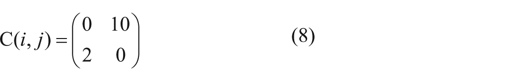
The values in the cost matrix were used to reflect the relative high cost of FN classifications after preliminary experimentation with different misclassification costs. These values were found to be satisfactory at reducing the FN rates without too great a cost being incurred in the increase of FP misclassifications, as was the case with higher ratios of costs for FP and FN. The performance of the various classification models using MetaCost are shown in Table 2 .

Table 2.

Performance of Classification Models Using MetaCost Cost Sensitivity.^a

Model	Accuracy (%)	Precision	Recall	F-Measure	ROC Area	Kappa	FP Rate	FN Rate
J48	96.11	0.965	0.961	0.962	0.957	0.8485	0.035	0.064
ADTree	91.42	0.944	0.914	0.922	0.974	0.7127	0.096	0.022
NBTree	96.63	0.97	0.966	0.967	0.99	0.8685	0.032	0.046
LMT	96.74	0.971	0.967	0.968	0.991	0.8728	0.031	0.043
ZeroOne	85.95	0.739	0.86	0.795	0.5	0	0	1
SMO	95.99	0.96	0.96	0.96	0.913	0.8328	0.022	0.151
Multilayer	85.95	0.739	0.86	0.795	0.5	0	0	1
REPTree	96.37	0.965	0.964	0.964	0.941	0.855	0.028	0.085
DecisionStump	94.84	0.949	0.948	0.949	0.902	0.7898	0.033	0.163
NaiveBayes	89.18	0.934	0.892	0.903	0.971	0.6534	0.12	0.035
RF (5 trees)	98.98	0.99	0.99	0.99	0.996	0.9593	0.011	0.004
RF (10 trees)	99.02	0.991	0.99	0.99	0.997	0.9606	0.011	0.001
RF (20 trees)	99.08	0.991	0.991	0.991	0.997	0.963	0.011	0
RF (50 trees)	99.09	0.991	0.991	0.991	0.998	0.9632	0.011	0

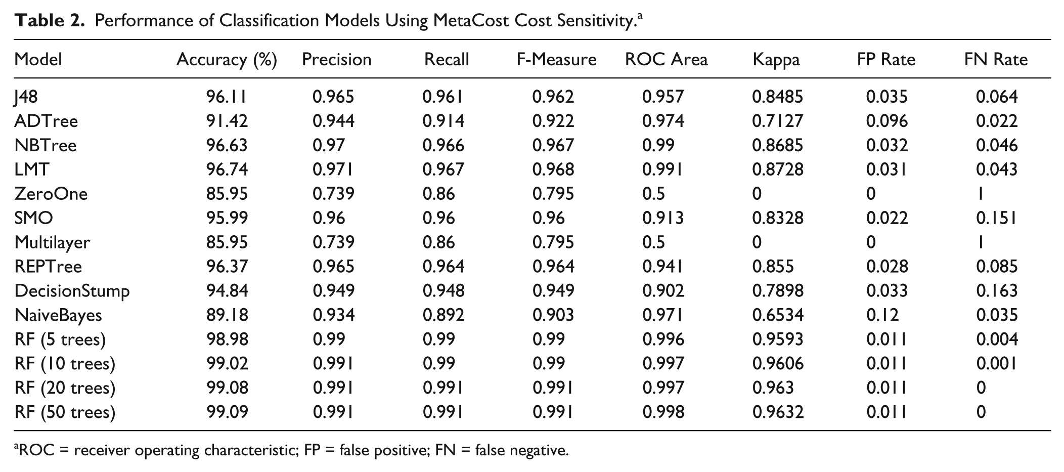
ROC = receiver operating characteristic; FP = false positive; FN = false negative.

The effect of applying the MetaCost wrapper to each classification model was assessed in terms of changes to the rates of FP and FN misclassifications. All the models show a significant reduction in FNR, with the exception of Decision Stump, for which the reduction in FNR was insignificant. In addition, RFs produced such low FNR with cost-insensitive models that any reduction by applying cost sensitivity was negligible. The most significant reduction was for ADTree, with an FNR of 0.14 for the cost-insensitive model and 0.022 using MetaCost. The application of MetaCost did incur a cost in terms of an increase in FPR; however, the increase in FPR was always lower than the decrease in FNR, with the exception of the Decision Stump algorithm. Again, the ADTree classifier showed the largest increase in FPR. The overall effect of cost sensitivity is summarized in Figure 4 showing the change in FPR and FNR for each model to which MetaCost was applied.

Figure 4.

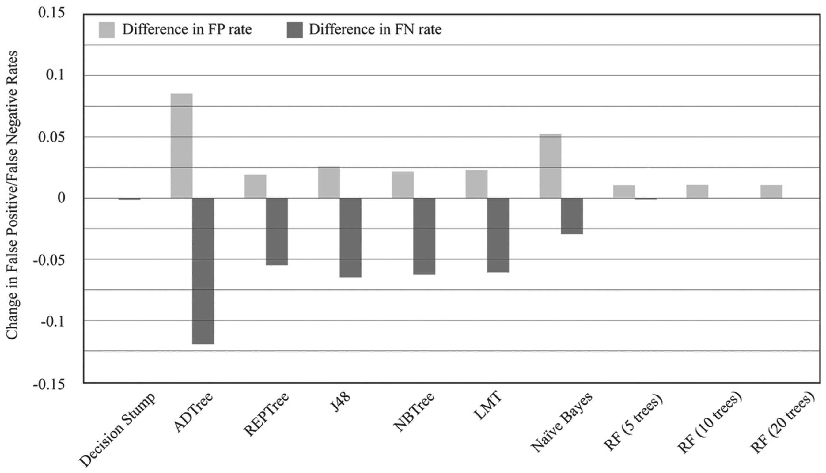
Changes in false-positive and false-negative rates for cost-insensitive and MetaCost classification models.

Variable Importance

Variable importance was assessed to establish which attributes were the most powerful at predicting the class outcome of analysis events. Chi-squared measurements were calculated and compared using JMP software package (JMP, SAS, Cary, NC). A classification and regression DT model was generated using JMP, similar to the SimpleCART implementation in WEKA. The contribution of each attribute to data partitioning was measured using the G² (likelihood-ratio chi-square). As expected, the two variables with the largest contribution to the class outcome were percent_purity_uv (748030.80) and horz_max_ms (240759.26), with get_cad_percent also scoring highly (47612.42). In addition, get_closest_peak and uv_peak_height made significant contributions to classification, with cad_start, retention_time and cad_stop also contributing to the partitioning of data. A notable finding in these results is the zero values for two of the criteria that were used to confirm an autopass in the previous LC-MS system, namely, uv_peak_width and cad_peak_area, suggesting that the inclusion of these two attributes in the previous autopass function is redundant. A table listing the G² value for each attribute is included in Supplementary Table S6.

Pruning and Model Stability

The results of applying the various pruning techniques are shown in Table 3 . All pruning methods greatly reduced the size and complexity of the DTs generated, with the exception of the LMT, which has a built-in pruning method that always generates compact models. Generally, the largest reduction in tree complexity was achieved by the minimum instances (minNum) prepruning method. Despite even the largest reduction in size and complexity, the pruned trees showed minor increases in accuracy, suggesting some degree of overfitting on training data for unpruned models.

Table 3.

Tree Complexity and Performance Using Different Pruning Methods.^a

Model	Accuracy (%)	Precision	Recall	F-Measure	ROC Area	Kappa	FP Rate	FN Rate
J48	96.11	0.965	0.961	0.962	0.957	0.8485	0.035	0.064
ADTree	91.42	0.944	0.914	0.922	0.974	0.7127	0.096	0.022
NBTree	96.63	0.97	0.966	0.967	0.99	0.8685	0.032	0.046
LMT	96.74	0.971	0.967	0.968	0.991	0.8728	0.031	0.043
ZeroOne	85.95	0.739	0.86	0.795	0.5	0	0	1
SMO	95.99	0.96	0.96	0.96	0.913	0.8328	0.022	0.151
Multilayer	85.95	0.739	0.86	0.795	0.5	0	0	1
REPTree	96.37	0.965	0.964	0.964	0.941	0.855	0.028	0.085
DecisionStump	94.84	0.949	0.948	0.949	0.902	0.7898	0.033	0.163
NaiveBayes	89.18	0.934	0.892	0.903	0.971	0.6534	0.12	0.035
RF (5 trees)	98.98	0.99	0.99	0.99	0.996	0.9593	0.011	0.004
RF (10 trees)	99.02	0.991	0.99	0.99	0.997	0.9606	0.011	0.001
RF (20 trees)	99.08	0.991	0.991	0.991	0.997	0.963	0.011	0
RF (50 trees)	99.09	0.991	0.991	0.991	0.998	0.9632	0.011	0

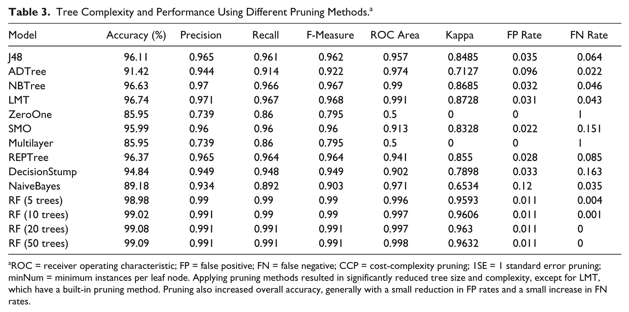
ROC = receiver operating characteristic; FP = false positive; FN = false negative; CCP = cost-complexity pruning; 1SE = 1 standard error pruning; minNum = minimum instances per leaf node. Applying pruning methods resulted in significantly reduced tree size and complexity, except for LMT, which have a built-in pruning method. Pruning also increased overall accuracy, generally with a small reduction in FP rates and a small increase in FN rates.

Discussion

The ideal scenario for quality assurance of large compound collections would be the existence of a universal method for identifying the structure and purity of research compounds. Although LC-MS is a ubiquitous technique for addressing this need, it is not a panacea for compound quality. Although most compounds can be successfully analyzed using this approach, there are a small minority of structures where this method is less effective. Ideally, an analyte would show a single, well-defined peak in the chromatography with high UV absorption. It would be successfully ionized and detected by MS, forming one of the simple adduct patterns for which the spectrometer has been programmed to look (the ionized molecules M+1 and M-1 and the sodiated ionized molecule M+23 included because of possible contaminants from glassware). This clear chromatographic separation of a single peak is rarely the case, with five integrated peaks being most common. The simplicity of the LC-MS results under investigation, compared with proteomics in which the integrated peaks can number in the hundreds,³¹ is confirmed by the fact that a brief review by a domain expert is often all that is required to confirm the outcome as a pass or fail. LC-MS results in this domain are clearly “solvable,” with even very simple rules such as Decision Stump showing high accuracy at predicting outcomes. It is, however, important to consider that most analyses produce multiple peaks, and only one peak per analysis can by definition be considered a pass, resulting in highly imbalanced data. An obviously useless model that predicted all peaks as fails would be correct in approximately 85% of cases. The real battleground for the development of high-performance classification models concerns the outliers at the fringe. Here the situation is more complex and requires more sophisticated algorithms that can examine the subtleties of the data to make accurate predictions. This has been successfully achieved by including the additional derived attributes and the use of more complex classification algorithms, such as ensemble methods.

As would be expected, the most powerful attributes for classifying results in this domain are the percent purity by UV and the spectral purity by MS (highest and second highest chi-squared values, respectively). In the original LC-MS system, three other attributes were used as supporting evidence of a pass result (UV peak height, UV peak width, and CAD peak area), with any analysis satisfying all five criteria labeled as an automatic pass. The philosophy applied to the original design of this process was deliberately cautious, and the inclusion of these five features was thought to provide strong evidence that the results of the analysis confirmed the purity and structural identity of the analyte. In addition, the threshold values applied to these features were set deliberately high, increasing the number of samples that would be diverted for manual review but minimizing the risk of FP classifications. Because of the generic nature of the detection methods used in this system, it was possible to produce FP results by detecting an analyte that coincidentally matched one of the adduct patterns but was in fact a different structure from the expected compound. It is also possible that a manually reviewed compound could be erroneously labeled as a pass during the review process. Both scenarios were considered infrequent, and the overall FP rate of the current LC-MS system, although difficult to quantify, was considered to be low.

The algorithms evaluated in this work confirm that the previous configuration was indeed cautious, particularly with regard to the value of spectral purity, which must have exceeded 30% for a sample to be considered a pass. The classification models generated often partitioned data on a figure of approximately 8% to 11% spectral purity, with further splitting on other attributes in lower nodes. When used in combination with these other attributes, these much lower values for spectral purity were found to be optimal at accurately classifying the data, supporting the assertion that the value of 30% used historically was indeed overly conservative. What is perhaps more interesting is that the most important variables that were found to contribute to the classification were not the five originally used in the autopass function but were derived attributes get_cad_percent and get_closest_peak. Although these attributes are applied to each peak individually, both have the characteristic of placing each peak in the context of the other peaks in an analysis event. The high chi-squared value for the get_closest_peak attribute suggests that it was successful in identifying peak integration errors, as discussed above and illustrated in Figure 1 . A large get_closest_peak increased the likelihood that a peak was predicted as a fail.

The ability of the RF model to make accurate predictions on the outcome of LC-MS analyses greatly increased the number of samples automatically processed compared with the previous system. An examination of 33,091 analyses that required manual review in the previous system but were automatically passed by the RF model (with a confidence ≥90%) revealed three main categories: (1) the sample passed the purity by UV criteria and the spectral purity criteria but failed one of the three additional tests on UV peak height, UV peak width, and CAD peak area (class label 3 of ms_pass_uv_pass_agreed_pass); (2) the sample passed purity by UV but failed the spectral purity filter (class label 3 of ms_fail_uv_pass_overwritten_pass); (3) the sample failed to reach the purity by UV criteria and passed the spectral purity criteria (class label 3 of ms_pass_uv_fail_overwritten_pass). The total numbers of analyses for these three categories are 19,481, 6437, and 7173, respectively.

The first category can be explained by the fact that of the three additional attributes, two (uv_peak_height and cad_peak_area) were found to make no significant contribution to the pass/fail outcome of an analysis, with uv_peak_height having some importance but scoring a relatively low value for G². Many of the reasons for these analyses not being automatically passed were therefore redundant and removed in the RF models. An example of this situation is provided in Supplementary Figure S6.

The second category could be explained by the observation discussed above that the original spectral purity threshold of 30% was overly cautious. Many analyses with a spectral purity of lower than 30% but higher than approximately 11% could be automatically flagged as passes in the RF model but not by the current LC-MS system. An example is provided in Supplementary Figure S7.

The third category may have a number of more complex explanations as a purity by UV lower than 85% would seem to indicate an impure sample and therefore a fail result. One explanation is that in some cases, the sample is eluted in the solvent front, meaning that it is not successfully recorded in the DAD chromatogram, which excludes the solvent front to avoid the dimethyl sulfoxide peak that would otherwise be detected. In such cases, an inspection by a domain expert could confirm this situation and enter an interpreted purity by UV, making the analysis result a pass. The RF model may be able to label an analyte as a pass if there is a strong signal in the CAD chromatogram, indicated by the derived attribute get_cad_percent. This demonstrates the utility of having a secondary detector in the LC-MS system. An example is given in Supplementary Figure S8.

In other cases, the peak integration performed by the instrument software may have split a single peak into two because of the presence of a “shoulder” in the chromatogram, as described earlier. The percent_purity_uv will be given for the incorrectly labeled portion of the actual peak and could therefore be less than 85%. The inclusion of additional derived attributes for get_cad_percent and get_closest_peak may allow the RF model to better identify occurrences of this type and correctly identify them as passed. An example of this is provided in Supplementary Figure S5.

The RF model generated a total of 335 FN misclassifications labeled auto_fail, with the remainder passing through for manual review. An examination of these results found that approximately 50% were due to the RF model making an incorrect decision on the outcome of the analysis, and the remaining 50% were due to the domain experts mislabeling the analyses as passed during the review stage. A common feature of many of the FN analyses is low-quality data, which could explain the high frequency of errors by domain experts during the review process. Many of these could be described as subjective or borderline with regard to the pass/fail outcome. An example is provided in Supplementary Figure S9. This analysis was marked as a pass by a domain expert because of the presence of the compound in the positive ion, albeit at low spectral purity because of the solvent front. Generally, the UV detection is the primary means of determining the pass/fail outcome of an analysis, but in this case, there was no significant UV signal. As there was no UV signal and a spectral purity of only 5.09%, the RF model labeled this analysis as a fail with high confidence (90%).

An analysis of the FP results revealed a number of categories: (1) the analysis was labeled by a domain expert as “no peaks,” indicating low confidence in the data generated (283 analyses, 14.4% of FPs); (2) the analysis was labeled as “no spectra” by the domain expert (298 analyses, 15.2% of FPs); (3) purity was overwritten with a value lower than 85% by a domain expert (347 analyses, 17.7% of FPs); (4) a value for “mass found” was entered by a domain expert, indicating that the compound detected did not have the expected mass (125 analyses, 6.4% of FPs); (5) no additional annotations by a domain expert but failed on spectral purity or purity by UV (913 analyses, 46.4% of FPs).

An example of category 1 FP is shown in Supplementary Figure S10. Both the percentage purity by UV and spectral purity have very high values and are passed by the RF model. The domain expert may have considered the UV signal to have been insufficient to pass this analysis (low UV peak height), preferring instead to trigger the sample to be reanalyzed by marking the results as “no peaks.” The calculated concentration from the CAD chromatogram is 1.54 mM rather than the expected 10 mM, indicating a possible injection issue. The results of the reanalysis are included in Supplementary Figure S11 and confirm the analysis as a pass. It could be said that the initial analysis was not necessarily a fail, but rather the domain expert did not consider the data provided enough confidence to pass the analysis, instead opting for it to be rerun.

An example of category 2 FP is shown in Supplementary Figure S12. A spectral purity of 18.49% and a purity by UV of 93.65% were sufficient for this analysis to be passed by the RF model. However, a visual inspection by a domain expert revealed a different interpretation. The large spectral peak at 390 Da in the positive ion mode suggests that the compound detected has a molecular mass of 389 Da and the 391 Da peak detected is the carbon 13 isotope rather than the ionized target compound.

An example of category 3 FPs is shown in Supplementary Figure S13. Again, the values for spectral purity and purity by UV of 42.39% and 100%, respectively, were sufficient for the RF model to label this analysis as an automatic pass. A comparison of the two chromatograms shows that the target compound exhibited low UV absorbance and all but one of the peaks integrated in the CAD were integrated in the UV. In response, the domain expert added an interpreted purity by UV of 65%, marking the result as a fail.

An example of category 4 FPs is shown in Supplementary Figure S14. In this example, the target mass is 239 Da. A spectral peak was detected as 240 Da, with a spectral purity of 5.49%. This may have been considered strong enough evidence for the RF model to label this result as a pass. A visual inspection by a domain expert again provided the correct interpretation. The large peak in the positive ion mode at 218 Da suggests the presence of a compound with a molecular weight of 217 Da. The peak at 240, therefore, is the sodiated ion M+23 and not the target compound. Further evidence of this is provided by the peak at 457 Da, which indicates the presence of 2M+23, the singly-sodiated dimer.

The remaining 46% of FPs all appear to have high values for spectral purity and purity by UV but not in excess of 30% and 85%, respectively, and so were marked as fails in the current system. These results are on the boundary between an automatic pass status and being diverted for review. Overall, the numbers are small, and as discussed previously, FP misclassifications are considered low cost. The number could be reduced by increasing the confidence level for automatic pass/fail but at a cost in terms of the number of analyses requiring manual review.

Many of the examples from the first four categories show the limitations of the RF model at accurately predicting the outcome of analyses. An obvious problem is detection being expressed as a percentage. One hundred percent of a poor-quality signal might be interpreted as strong evidence of a pass by the RF model but would not be considered a high-confidence result by a domain expert, preferring to repeat the analysis. Other issues arise from the simplicity of the method of detection by spectral purity. As each peak is considered individually, none of the data-mining algorithms are capable of recognizing the kinds of patterns and signatures shown in the category 4 example (Suppl. Fig. S14), which would require a review by an experienced technician.

Despite these limitations, the relatively small FPR offset against the reduction in manual reviews was still considered a significant improvement from the current LC-MS system. At a steady state of approximately 25,000 results per month, the estimated time spent reviewing data is 15 h/wk or 40% of a full-time employee. The application of the RF model using a confidence threshold of 90% on predictions would reduce this time from 15 h to 8.25 h, or from 40% of one full-time employee to 22%. This reduction could potentially be recouped in two ways: an annual saving of $45,000 in reduced staff requirements and a potential increase in the capacity of the LC-MS system from the current rate of 25,000 analyses per month up to 45,000 with the same resource levels.

All classification models were able to make accurate predictions on LC-MS outcomes, with RF generated with WEKA showing the best performance, with an accuracy close to 100%. The RFs generated with Pipeline Pilot were less accurate (10 tree RF was 96.06% accurate with an F-measure of 0.873) but had the advantage of generating confidence measures on predictions.

The application of MetaCost reduced the FNR more than it increased the FPR for all models except Decision Stump, Naive Bayes where the increase in FPR was larger than the decrease in FNR, and the RFs, where the FNR was already very low.

Variable importance measurements suggested that percent_purity_uv (purity by UV) and horz_max_ms (spectral purity by MS) were the most important variables in determining the outcome of an analysis. The derived attributes get_cad_percent and get_closest_peak made the third and fourth largest contribution, respectively, to determining the outcome. The prepruning method of a minimum number of instances per leaf node greatly reduced the size and complexity of DTs without reducing and in some cases increasing accuracy.

The predictions of LC-MS outcomes sought in this work are binary decisions of pass or fail. Although achieving the objective of reducing the number of manual reviews, this does come at a cost; the models are not capable of distinguishing the different reasons for failures. However, simple methods could be applied to make some distinctions. For example, autofails where a peak had a high value for purity by UV would indicate a substance was found but was not the expected mass. This differs from autofails where no substance was detected. Furthermore, if there were no integrated peaks in the results, or if all were of particularly low quality (very low spectral purity), this may indicate that the analysis itself has failed, a different situation from the analysis being performed and producing a fail outcome. Rather than being flagged as requiring a manual review, these analyses could be marked as erroneous results, triggering a second analysis of the sample. This approach would further reduce the number of analyses requiring manual review and be another step toward a highly automated, high-performance system for quality assurance by LC-MS.

Footnotes

Acknowledgements

The author would like to thank Professor John Keane (University of Manchester) for expert advice on the use and evaluation of data-mining algorithms, Ian Sinclair (AstraZeneca) and Sunil Sarda (AstraZeneca) for technical expertise on LC-MS, and Ian Sunil and Dr Clive Green (AstraZeneca) for help and advice editing this article.

Supplementary material for this article is available on the Journal of Laboratory Automation Web site at .

Declaration of Conflicting Interests

The author declared no potential conflicts of interest with respect to the research, authorship, and/or publication of this article.

Funding

The author received no financial support for the research, authorship, and/or publication of this article.

References

Kyranos

J. N.

Cai

Wei

High-Throughput High-Performance Liquid Chromatography/Mass Spectrometry for Modern Drug Discovery. Curr. Opin. Biotechnol. 2001, 12, 105–111.

Duléry

B. D.

Verne-Mismer

Wolf

. Analyses of Compound Libraries Obtained by High-Throughput Parallel Synthesis: Strategy of Quality Control by High-Performance Liquid Chromatography, Mass Spectrometry and Nuclear Magnetic Resonance Techniques. J. Chromatogr. B. Biomed. Sci. Appl. 1999, 725, 39–47.

Sinclair

Charles

Applications of the Charged Aerosol Detector in Compound Management. J. Biomol. Screen. 2009, 14, 531–537.

Yates

Compound Management Comes of Age. Drug Discovery World 2003, Spring, 35–42.

Comley

Nanolitre Dispensing. Drug Discovery World 2004, Summer, 43–54.

Chen

Pramanik

B. N.

Liu

Y. H.

Applications of LC/MS in Structure Identifications of Small Molecules and Proteins in Drug Discovery. J. Mass. Spectrom. 2007, 42, 279–287.

Süßmuth

R. D.

Jung

Impact of Mass Spectrometry on Combinatorial Chemistry. J. Chromatogr. B. Biomed. Sci. Appl. 1999, 725, 49–65.

Charles

Sinclair

Addison

D. H.

Capture and Exploration of Sample Quality Data to Inform and Improve the Management of a Screening Collection. J. Lab. Autom. 2014, 19, 198–207.

Markey

M. K.

Tourassi

G. D.

Floyd

C. E.

Jr.

Decision Tree Classification of Proteins Identified by Mass Spectrometry of Blood Serum Samples from People with and without Lung Cancer. Proteomics 2003, 3, 1678–1679.

10.

Shen

Qian

. Diagnosis of Gastric Cancer Using Decision Tree Classification of Mass Spectral Data. Cancer Sci. 2007, 98, 37–43.

11.

Abbott

Fishman

. Comparison of Statistical Methods for Classification of Ovarian Cancer Using Mass Spectrometry Data. Bioinformatics 2003, 19, 1636–1643.

12.

Burbidge

Trotter

Buxton

. Drug Design by Machine Learning: Support Vector Machines for Pharmaceutical Data Analysis. Comput. Chem. 2001, 26, 5–14.

13.

Dettmer

Aronov

P. A.

Hammock

B. D.

Mass Spectrometry-Based Metabolomics. Mass Spectrom. Rev. 2007, 26, 51–78.

14.

Yates

J. R.

Ruse

C I.

Nakorchevsky

Proteomics by Mass Spectrometry: Approaches, Advances, and Applications. Annu. Rev. Biomed. Eng. 2009, 11, 49–79.

15.

Yates

J. R.

III . Mass Spectrometry: From Genomics to Proteomics. Trends Genet. 2000, 16, 5–8.

16.

Hall

Frank

Holmes

. The WEKA Data Mining Software: An Update. ACM SIGKDD Explorations Newsletter 2009, 11, 10–18.

17.

Domingos

MetaCost: A General Method for Making Classifiers Cost-Sensitive, Proceedings of the Fifth ACM SIGKDD International Conference on Knowledge Discovery and Data Mining; ACM: New York, 1999; pp 155–164.

18.

Eriksson

Glansberg

Jörtsö

Cost-Sensitive Classifiers. Linköping University [Online] 2009. http://webstaff.itn.liu.se/~aidvi/courses/06/dm/Seminars2009/P-Cost-sensitive%20Classifiers.pdf (accessed Dec 2, 2014).

19.

Kullback

Leibler

R. A.

On Information and Sufficiency. Ann. Math. Statist. 1951, 22, 79–86.

20.

Gini

Variabilità e mutabilità. Memorie di metodologica statistica, 1912.

21.

Quinlan

J. R.

Simplifying Decision Trees. Int. J. Man-Mach. Stud. 1987, 27, 221–234.

22.

Olshen

L. B. J. F. R.

Stone

C. J.

Classification and Regression Trees. Wadsworth Int. Group 1984, 101.

23.

Opitz

Maclin

Popular Ensemble Methods: An Empirical Study. J. Artif. Intell. Res. 1999, 11, 169–198.

24.

Breiman

Bagging Predictors. Machine Learn. 1996, 24, 123–140.

25.

Freund

Schapire

R. E.

Experiments with a New Boosting Algorithm. In Machine Learning, Proceedings of the Thirteenth International Conference; 1996, 96, 148–156.

26.

Breiman

Random Forests. Machine Learn. 2001, 45, 5–32.

27.

Wolpert

Stacked Generalization. Neural Netw. 1992, 5, 241–259.

28.

Famili

Phan

Fauteux

. Data Integration and Knowledge Discovery in Life Sciences, IEA/AIE’10 Proceedings of the 23rd International Conference on Industrial, Engineering and Other Applications of Applied Intelligent Systems; García-Pedrajas

., Eds.; Springer: Berlin, 2010, pp 102–111.

29.

Robnik-Šikonja

Improving Random Forests. In Machine Learning, ECML 2004 Proceedings; Springer: Berlin, 2004, pp 359–370.

30.

Oshiro

T. M.

Perez

P. S.

Baranauskas

J. A.

How Many Trees in a Random Forest? In Machine Learning and Data Mining in Pattern Recognition, ser. Lecture Notes in Computer Science; Perner

, Ed.; Springer: Berlin, 2012, pp 154–168.

31.

Bern

Goldberg

McDonald.

W. H.

. Automatic Quality Assessment of Peptide Tandem Mass Spectra. Bioinformatics 2004, 20(suppl 1), i49–i54.

Toward Automated Interpretation of LC-MS Data for Quality Assurance of a Screening Collection

Abstract

Keywords

Introduction

Methods

Pruning

Ensemble Methods of Classification

Results

Evaluation of Classification Models

Cost-Sensitive Classification Using MetaCost

Variable Importance

Pruning and Model Stability

Discussion

Footnotes

Acknowledgements

Declaration of Conflicting Interests

Funding

References