Sage Journals: Discover world-class research

Abstract

Protein–protein interactions (PPIs) provide valuable insight into the inner workings of cells, and it is significant to study the network of PPIs. It is vitally important to develop an automated method as a high-throughput tool to timely predict PPIs. Based on the physicochemical descriptors, a protein was converted into several digital signals, and then wavelet transform was used to analyze them. With such a formulation frame to represent the samples of protein sequences, the random forests algorithm was adopted to conduct prediction. The results on a large-scale independent-test data set show that the proposed model can achieve a good performance with an accuracy value of about 0.86 and a geometric mean value of about 0.85. Therefore, it can be a usefully supplementary tool for PPI prediction. The predictor used in this article is freely available at http://www.jci-bioinfo.cn/PPI_RF.

Keywords

physicochemical descriptor wavelet transform random forest protein–protein interaction

Introduction

Proteins play a vital role in nearly all biological functions, such as composing the cellular structure and promoting chemical reactions. Many critical functions and processes in biology are sustained largely by different types of protein–protein interactions (PPIs), and PPIs are highly relevant to disease states. During the past few years, a vast amount of protein data has received a significant improvement with the rapid development of biotechnology. In recent years, various experimental techniques have been developed for large-scale PPI analysis, such as yeast two-hybrid systems,^1,2 mass spectrometry,^3,4 protein chips,⁵ and so on. But these experimental approaches are tedious, time-consuming, labor-intensive, and expensive.⁶ Only a small part of the PPIs’ pairs is analyzed by such methods.⁶ Hence, it is important to develop a reliable computational model to relieve the difficulty of the identification of PPIs.

In biology, it is virtually axiomatic that the sequence specifies conformation, which implies an intriguing hypothesis: The amino acid sequence alone might be sufficient to determine the conformation of the protein.⁷ Therefore, only the sequence information may be used to predict the interactions between two proteins via machine learning methods. Until now, a number of computational models have been proposed for predicting PPIs using simple protein sequence information alone,^8–13 and some impressive performances have been reported. Some methods based on the genomic information, such as phylogenetic profiles,^14,15 the gene neighborhood,¹⁶ and gene fusion events,^17,18 have been developed for prediction of PPIs by accounting for the pattern of the presence or absence of a given gene in a set of genomes. But they can be applied only to completely sequenced genomes and cannot be used for the essential protein that is common to most organisms. Sequence conservation ^19,20 between interacting proteins also has been reported. Martin et al.²¹ and Chou²² et al. have developed computational methods for PPIs identification only via the sequence information and have had a prediction accuracy of 80%. Shen et al.⁹ have developed an improved model that reaches a higher prediction accuracy of 83.5% when applied to human PPI identification. All of these methods account for the properties of one amino acid and its proximate two amino acids via a conjoint triad method. In fact, the PPIs may occur in the discontinuous amino acids segments in the sequence, and the prediction ability of these sequence-based methods may be beneficial from the consideration of these interactions. Furthermore, the prediction models used in these methods were developed via limited training samples (often, <3000 protein pairs) but with hundreds of variants. Therefore, they can easily encounter the overfitting problem, and the results are data dependent.

In this study, a new method based on the random forests algorithm and discrete wavelet transform (DWT)²³ with several physiochemical descriptors was proposed. To avoid the problem of overfitting, more than 10,000 PPIs were used to train the prediction model. The method was composed of three main steps. First, the protein sequences were converted into numerical signals by using the physicochemical properties of amino acids, and then these sequences were further analyzed by DWT, through which further relationships of the protein residues were considered. Second, the salient frequency-band features of DWT were extracted, and a series of statistical features was used to construct the feature vectors for representation of the protein sequence. Finally, the random forests algorithm²⁴ was applied to deal with the classified problem of PPI identification using these statistical feature vectors as inputs. The predictive results of the cross-validation test show that the proposed method is effective.

Materials and Methods

Data Collection and Data Set Construction

To develop a PPI prediction model, we need to construct or select a valid benchmark data set with which to train and test the predictor. The PPI data used in this article were collected from the publicly available Saccharomyces cerevisiae and Helicobacter pylori data sets.

In our experiments, a yeast (S. cerevisiae) data set is first used in independent study, which was downloaded from the Database of Interacting Proteins (DIP; version 20140703).²⁵ This data set contains 22,775 positive pairs. The protein pairs that contain a protein with fewer than 50 amino acids are removed, and then a nonredundant subset is generated at the sequence identity level of 40% by cluster analysis of the CD-HIT program.²⁶ After these pre-processing procedures, the total positive data set is reduced to 17,505.

Because the non-interacting pairs are not readily available from DIP, we construct them by using the following methods. The negative data set is generated based on the assumption that proteins locating different subcellular localizations do not interact. The subcellular location information of the proteins was extracted from Swiss-Prot (http://www.expasy.org/sprot/). The positive data may be divided into several types of localization—cytoplasm, nucleus, mitochondrion, endoplasmic reticulum, Golgi apparatus, peroxisome, and vacuole. The negative data were obtained by pairing proteins from one location with proteins from other ones. The strategies must meet the following requirements:^9,10 (1) the non-interacting pairs cannot appear in the positive data set; and (2) the contribution of proteins in the negative set should be as harmonious as possible. A total of 5943 negative pairs were generated via this approach.

However, Ben-Hur and Noble²⁷ have pointed out that the restricting negative examples of different sublocation pairs lead to a biased estimate of the accuracy of a PPI predictor. So it is necessary to generate negative pairs with the same localization to reduce the effects of the bias. The protein pairs at the same localization are considered as the negative pairs if none of them has occurred in the yeast-positive pairs. From the seven sublocalizations, 27,204 negative pairs are generated (8000 at the cytoplasm, 8000 at the nucleus, 8284 at the mitochondrion, 1953 at the endoplasmic reticulum, 300 at the Golgi apparatus, 171 at the peroxisome, and 496 at the vacuole).

The H. pylori data set is composed of 2916 protein pairs (1458 positive pairs and 1458 negative pairs) as described by Maritin.²¹ This data set was used to test the sensitivity of the parameters of the model, and it gives a comparison of our predictor with other ones.

Feature Extraction

One important step to predict PPIs by using sequence information is to find a suitable encoding of the protein sequence. This means converting the protein sequence to a vector space. In this article, the physicochemical properties of amino acids were selected to translate a protein sequence to seven vectors. The seven physicochemical descriptors are hydrophobicity,²⁸ hydrophicility,²⁹ volumes of side chains of amino acids,³⁰ polarity,³¹ polarizability,³² solvent-accessible surface area (SASA),³³ and the net charge index (NCI) of side chains of amino acids.³⁴ The original values of the seven descriptors for each amino acid are listed in Table 1 . We first normalized them to zero mean and unit standard deviation according to the following equation:

P_{i j}^{'} = \frac{P_{i, j} - P_{j}}{S_{j}}

where P_i,j is the jth descriptor value for the ith amino acid; P_j is the mean of the jth descriptor over the 20 amino acids; and S_j is the corresponding standard deviation.

Table 1.

The Original Values of the Seven Physicochemical Properties for Each Amino Acid.

Code	H1	H2	V	P1	P2	SASA	NCI
A	0.620	−0.500	27.500	8.100	0.046	1.181	7.187 × 10⁻³
C	0.290	−1.000	44.600	5.500	0.128	1.461	−3.661 × 10⁻²
D	−0.900	3.000	40.000	13.000	0.105	1.587	−2.382 × 10⁻²
E	−0.740	3.000	62.000	12.300	0.151	1.862	6.802 × 10⁻³
F	1.190	−2.500	115.500	5.200	0.290	2.228	3.755 × 10⁻²
G	0.480	0.000	0.000	9.000	0.000	0.881	1.791 × 10⁻¹
H	−0.400	−0.500	79.000	10.400	0.230	2.025	−1.069 × 10⁻²
I	1.380	−1.800	93.500	5.200	0.186	1.810	2.163 × 10⁻²
K	−1.500	3.000	100.000	11.300	0.219	2.258	1.771 × 10⁻²
L	1.060	−1.800	93.500	4.900	0.186	1.931	5.167 × 10⁻²
M	0.640	−1.300	94.100	5.700	0.221	2.034	2.683 × 10⁻³
N	−0.780	2.000	58.700	11.600	0.134	1.655	5.392 × 10⁻³
P	0.120	0.000	41.900	8.000	0.131	1.468	2.395 × 10⁻¹
Q	−0.850	0.200	80.700	10.500	0.180	1.932	4.921 × 10⁻²
R	−2.530	3.000	105.000	10.500	0.291	2.560	4.359 × 10⁻²
S	−0.180	0.300	29.300	9.200	0.062	1.298	4.627 × 10⁻³
T	−0.050	−0.400	51.300	8.600	0.108	1.525	3.352 × 10⁻³
V	1.080	−1.500	71.500	5.900	0.140	1.645	5.700 × 10⁻²
W	0.810	−3.400	145.500	5.400	0.409	2.663	3.798 × 10⁻²
Y	0.260	−2.300	117.300	6.200	0.298	2.368	2.360 × 10⁻²

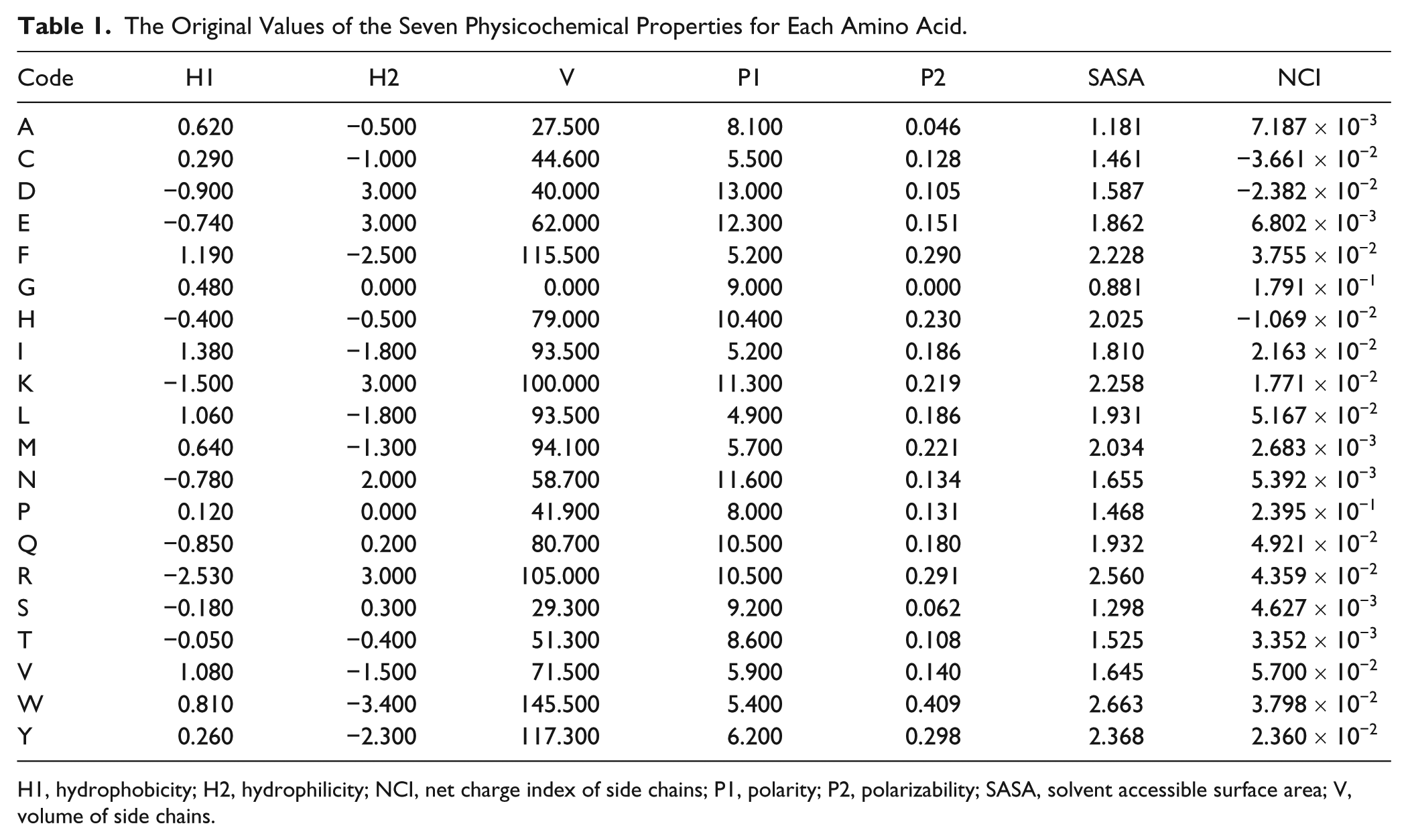
H1, hydrophobicity; H2, hydrophilicity; NCI, net charge index of side chains; P1, polarity; P2, polarizability; SASA, solvent accessible surface area; V, volume of side chains.

After we obtained these seven vectors, they were regarded as seven digital signals. Discrete wavelet transform was used to deal with them. Wavelet transform is a multiresolution analysis tool.³⁵ It has become very popular when it comes to analysis, and de-noising and compressing signals and images. Wavelet transform decomposes a signal into a set of basic functions. These basic functions are called wavelets. Wavelets are obtained from a single prototype wavelet-call mother wavelet by dilations and shifting:

Ψ_{a, b} (t) = \frac{1}{\sqrt{a}} Ψ (\frac{t - b}{a})

where $Ψ (t)$ is the mother wavelet; a is the scaling parameter; and b is the shifting parameter. The one-dimensional (1D) wavelet transform is given by:

W_{f} (a, b) = \int_{- \infty}^{\infty} x (t) Ψ_{a, b} (t) d t

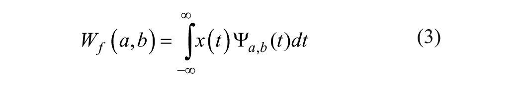
where x(t) is the decomposed signal. DWT transforms discrete time signals to a discrete wavelet representation. It converts an input series X₀, X₁,… X_n into one high-pass wavelet coefficient series and one low-pass wavelet coefficient series (of length m/2 each), given by, respectively:

H_{p} = \sum_{m = 0}^{k - 1} X_{2 p - m} . s_{m} (Z)

L_{p} = \sum_{m = 0}^{k - 1} X_{2 p - m} . t_{m} (z)

where $s_{m} (Z)$ and $t_{m} (Z)$ are called wavelet filters; k is the length of the filter; and $p = 0, \dots, [\frac{n}{2}] - 1$ . In practice, such transforms will be applied recursively on the low-pass series using the Mallat algorithm³⁶ until the desired number of iterations is reached. The block diagram in Figure 1 depicts the digital implementation of DWT.

Figure 1.

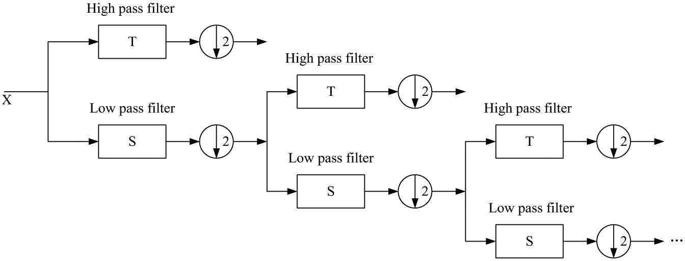
Procedure of multilevel discrete wavelet transform (DWT). Three levels of DWT are shown in the figure, and we can get four subbands.

After the decomposition of the seven vectors via DWT, the wavelet coefficients can be used as the protein feature vector. But if we did it like this, an overfitting problem from the vast feature vector will occur. To further reduce the dimensionality of the feature vectors, statistics were used over the set of the wavelet coefficients of each subband. The following statistical features of each subband were used for the prediction of PPIs:

(1) Maximum of the wavelet coefficients in subband q

m a x_{q} = m a x (e_{q})

(2) Mean of the wavelet coefficients in subband q

a v g_{q} = \sum (e_{q}) / n_{q}

(3) Minimum of the wavelet coefficients in subband q

m i n_{q} = m i n (e_{q})

(4) Standard deviation of the wavelet coefficients in subband q

s t d_{q} = \sqrt{\frac{1}{n_{q}} \sum {(e_{q} - a v g_{q})}^{2}}

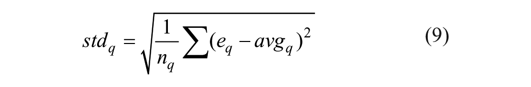
where e_q is the wavelet coefficients at the subband q; and n_q is the number of wavelet coefficients at the subband q. This method is the same as the random subspace approach, especially in the aspect of selecting the optimal feature vector. In this article, the decomposition level λ = 4, which is similar to that in Ref.³⁷, was selected to represent a protein for prediction of PPIs, and a 20-dimensional feature vector can be obtained for each protein descriptor vector. Finally, a 20×7×2 dimensional feature vector, where 7 was the number of physicochemical descriptors used in our study and 2 was the number of proteins included in PPI pairs, was input to the learning system for prediction.

Random Forests Algorithm

Random forests algorithm, developed by Leo Breiman,²⁴ is an ensemble of unpruned classification and regression trees that operates by constructing a multitude of decision trees at the training time and outputting the final class that is the majority vote of the classes output by individual trees. These trees are generated by bootstrap samples of the training data and by using random feature selection in the tree generation process. Random forests algorithm usually exhibits a remarkable improvement of performance compared to single decision tree classifiers such as CART and C4.5,³⁸ which are often used as the base learner in random forests algorithm. Furthermore, random forests algorithm shows a good generalization error rate when compared to Adaboost and is more robust to noise. In our experiments, 200 trees are used in our model as the computational cost and overfitting problem are considered. The schematic diagram of the proposed method is shown in Figure 2 .

Figure 2.

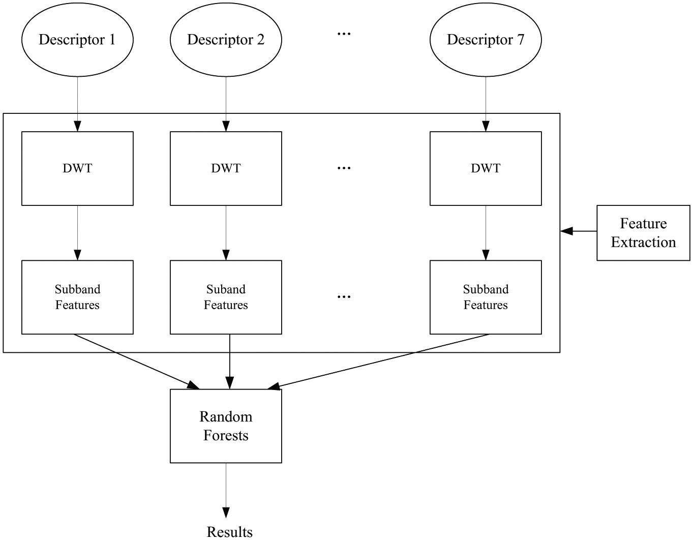
Framework of the proposed framework. Seven physicochemical descriptors and discrete wavelet transform (DWT) are used to describe the protein. Random forests algorithm is used for prediction.

Evaluation Measures

In the literature, six metrics were often used to score the quality of a predictor at seven different angles; these include accuracy (Acc), sensitivity (Sen), specificity (Spec), and the F-measure (Fm). These measures are defined in Table 2 . Sensitivity (Sen) and specificity (Spec) illustrate the correct prediction ratios of positive and negative data sets, respectively. The overall accuracy (Acc) is measured as the average of sensitivity (Sen) and specificity (Spec). But when the numbers of positive data and negative data differ too much from each other, the Mathew correlation coefficient (MCC) should be calculated to assess the prediction performance. The value of MCC ranges from −1 to 1, and a bigger MCC stands for better prediction performance.

Table 2.

Evaluation Measurements.

Measurements	Abbreviation	Equation
Accuracy	Acc	(TP + TN) / (TP + TN + FP + FN)
Sensitivity	Sen	TP / (TP + FN)
Specificity	Spec	TN / (TN + FN)
F-measure	Fm	2TP / (2TP + FP + FN)
Mathew correlation coefficient	Mcc	$\frac{TP * TN - FN * FP}{\sqrt{(TP * FN) * (TN * FP) * (TP * FP) * (TN * FN)}}$
Geometric mean	GM	sqrt{[TP / (TP + FP)] * [TN / (TN + FN)]}

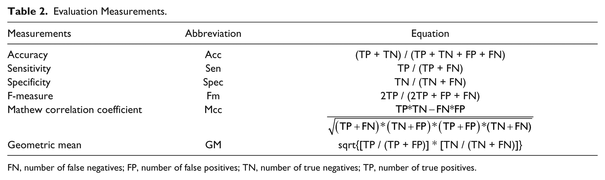
FN, number of false negatives; FP, number of false positives; TN, number of true negatives; TP, number of true positives.

With a set of clear and valid metrics as defined in Table 2 to measure the quality of a predictor, the next thing we need to consider is how to objectively derive the values of these metrics for a predictor.

In statistical prediction, the following three cross-validation methods are often used to calculate the metrics in Table 2 for evaluating the quality of a predictor: an independent data set test, a subsampling (e.g., 2-, 5-, or 10-fold cross-validation) test, and a jackknife test. The jackknife test was deemed the least arbitrary; it can always yield a unique result for a given benchmark data set. Therefore, the jackknife test has been increasingly and widely adopted by investigators to test the power of various prediction methods. However, to reduce the computational time, we adopted the 5-fold cross-validation or 10-fold cross-validation in this study that was performed by many investigators with random forests algorithm as the prediction engine. In k-fold cross-validation, the original sample is randomly partitioned into k subsamples. Of the k subsamples, a single subsample is retained as the validation data for testing the model, and the remaining subsamples are used as training data. The cross-validation process is then repeated k times (the folds), with each of the k subsamples used exactly once as the validation data. The advantage of this method is that all observations are used for both training and validation; it has high computational efficiency and thus has been used often in protein attributes prediction model checking. However, as can be seen, because the partition is random, the result is variable.

Web Server and User Guide

To enhance the value of the PPI predictor’s practical applications, a web server for it was established at http://www.jci-bioinfo.cn/PPI_RF. Moreover, for the convenience of the vast majority of experimental scientists, a step-to-step guide is provided here for how to use the web server predictor:

Step 1: Go to http://www.jci-bioinfo.cn/PPI_RF, and you will see the top page of the predictor on your computer screen, as shown in Figure 3 . Click on Read Me to see a brief introduction about the PPI predictor.

Step 2: When the predicted PPIs are only in several protein sequences, you can either type or copy/paste the query protein sequence into the input box at the top half of Figure 3 . It is important to note that the input sequence should be in the FASTA format. A sequence in FASTA format consists of a single initial line beginning with a greater-than symbol (>) in the first column, followed by lines of sequence data. The words right after the > symbol in the single initial line are optional and only used for the purposes of identification and description.

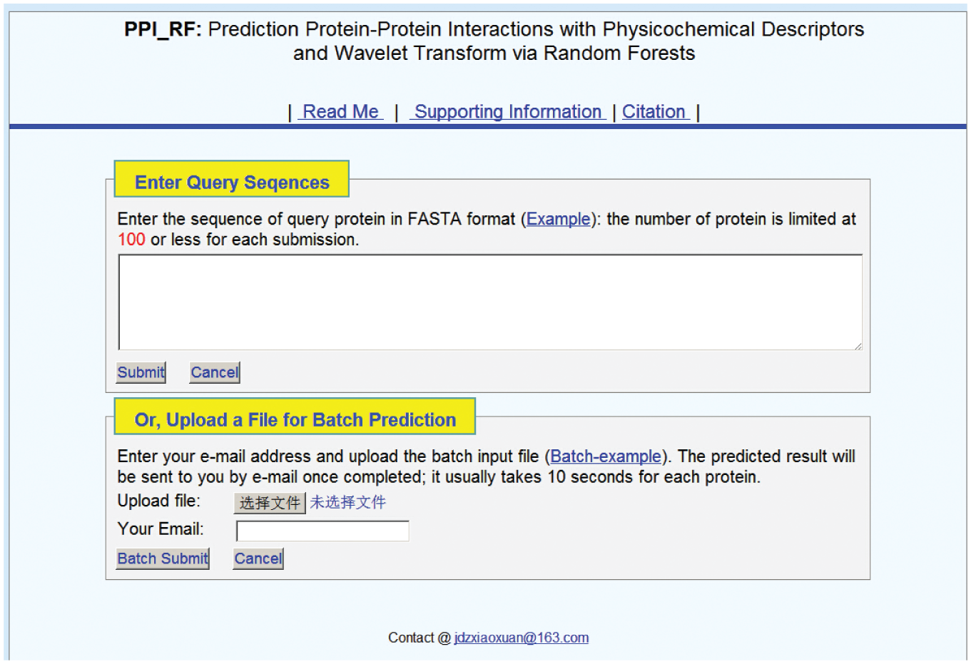
Step 3: To get the predicted result, you only need to click on the Submit button. For example, if you use the query amino acids sequences in the Example window as input, you will see the status of your job on your screen. When the job is done, the results will be displayed on the page.

Figure 3.

Screenshot of the PPI Predictor Web Server.

As regards the computational time, the work will be accomplished within 15s in most cases. However, the length of the sequence is the key crucible for time consumption; the longer the query protein sequence is, the more time is usually needed.

Step 4: As shown in the lower panel of Figure 3 , you may also choose batch prediction by entering your e-mail address and your desired batch input file (in FASTA format) via the Browse button. To see a sample of a batch input file, click on the Batch-Example button.

Step 5: By clicking the Citation button, you will find the relevant papers that document the detailed development of the predictor.

Step 6: Click on the Supporting Information button to download the benchmark data set used to train and test the PPI predictor.

Results and Discussion

Effect of Wavelet Functions

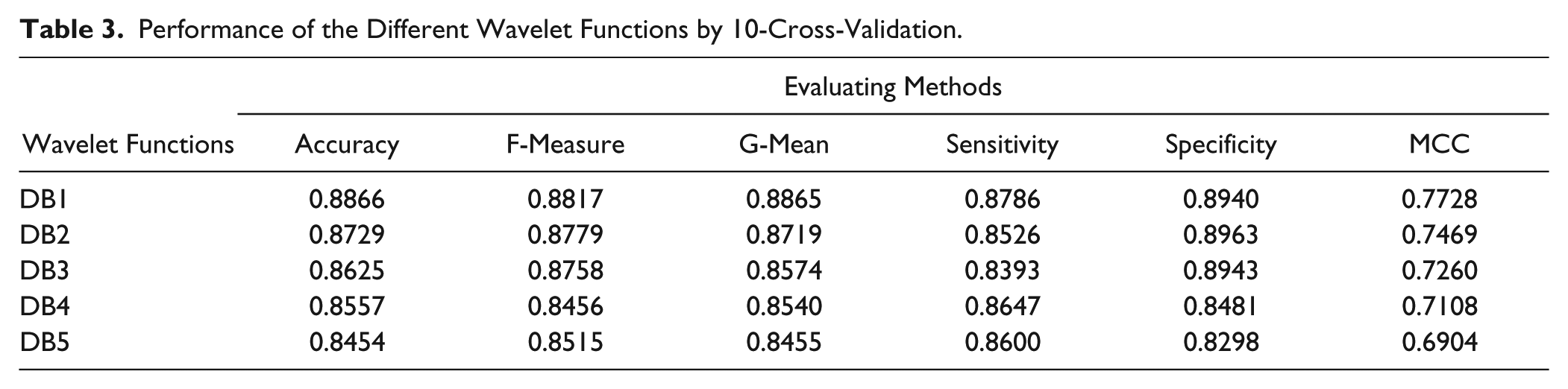
In this section, the influence of the wavelet function was analyzed because a suitable wavelet basis can match the underlying structure of the signal better, and better features can be extracted from the original protein sequences. Some properties of the wavelet basis, such as compact support, orthogonality, symmetry, smoothness, and a high order of vanishing moments, must be considered for signal processing. It is hoped that the wavelet functions would own these mentioned properties. However, there are many conflicting conditions that restrict the selection of them. None of the wavelet basis functions possesses all of these desirable properties simultaneously. In recent decades, Daubechies constructed a class of orthonormal wavelet basis functions with compact support and smooth properties. In this study, five Daubechies²³ were tested: Daubechies of number 1 (Db1), number 2 (Db2), number 3 (Db3), number 4 (Db4), and number 5 (Db5). As seen in Table 3 , the training accuracy reached 0.8542 when using the random forests algorithm as the classifier with the DB1 wavelet function used to extract the features. The number of trees in random forests is 200, and the number of mtrys (dimension of subspace) is 45. However, when other wavelet functions are used, the training accuracies range from 0.8454 to 0.8866. Moreover, other performance measures, such as geometric means, sensitivity, specificity, F-measure, and MCC, were also investigated. Table 3 shows that DB1 was also the best one. These results may be caused by a property that the DB1 wavelet possesses: a lower vanish moment. More non-zero coefficients are generated after the decomposition, and the diverse trees used in random forests are easy obtained because the diversity of component learners is necessary.⁴⁰ But for a single learner, a higher-vanish-moment wavelet function such as DB4 is needed. In this study, the DB1 wavelet function was selected as the appropriate wavelet function in our experiments.

Table 3.

Performance of the Different Wavelet Functions by 10-Cross-Validation.

	Evaluating Methods
Wavelet Functions	Accuracy	F-Measure	G-Mean	Sensitivity	Specificity	MCC
DB1	0.8866	0.8817	0.8865	0.8786	0.8940	0.7728
DB2	0.8729	0.8779	0.8719	0.8526	0.8963	0.7469
DB3	0.8625	0.8758	0.8574	0.8393	0.8943	0.7260
DB4	0.8557	0.8456	0.8540	0.8647	0.8481	0.7108
DB5	0.8454	0.8515	0.8455	0.8600	0.8298	0.6904

Performance on the S. cerevisiae Data Set

The proposed predictor was first applied to the S. cerevisiae data set. The data set consisted of 17,505 positive pairs and 27,204 negative pairs; 5943 positive pairs and 5943 negative pairs were randomly selected from S. cerevisiae as the training data set. The remained ones were used as the independent-test data set. A 5-fold cross-validation was used to evaluate the predictor on the training data set, and the procedure was repeated 10 times. The results from the training data set are shown in Table 4 .

Table 4.

5-fold Cross-Validation Results of the Training Data on the S. cerevisiae Data Set.

	Evaluation Methods
	Accuracy	Sensitivity	Specificity	F-Measure	MCC	G-Mean
1	0.8376±0.0035	0.8607±0.0114	0.8174±0.0098	0.8322±0.0044	0.6768±0.0072	0.8371±0.0036
2	0.8384±0.0069	0.8597±0.0097	0.8195±0.0097	0.8334±0.0080	0.6780±0.0137	0.8379±0.0071
3	0.8349±0.0048	0.8538±0.0134	0.8182±0.0088	0.8304±0.0055	0.6710±0.0101	0.8345±0.0049
4	0.8429±0.0058	0.8656±0.0099	0.8228±0.0148	0.8379±0.0057	0.6873±0.0109	0.8425±0.0056
5	0.8417±0.0030	0.8677±0.0110	0.8191±0.0072	0.8358±0.0059	0.6852±0.0068	0.8410±0.0037
6	0.8336±0.0031	0.8596±0.0069	0.8111±0.0065	0.8273±0.0046	0.6690±0.0061	0.8328±0.0034
7	0.8359±0.0083	0.8610±0.0138	0.8141±0.0171	0.8300±0.0080	0.6736±0.0160	0.8353±0.0081
8	0.8412±0.0064	0.8622±0.0116	0.8231±0.0144	0.8366±0.0068	0.6840±0.0123	0.8407±0.0065
9	0.8382±0.0100	0.8617±0.0073	0.8181±0.0195	0.8328±0.0110	0.6782±0.0184	0.8376±0.0101
10	0.8401±0.0055	0.8635±0.0138	0.8195±0.0070	0.8348±0.0055	0.6816±0.0116	0.8395±0.0053
mean	0.8395±0.0029	0.8615±0.0036	0.8183±0.0034	0.8331±0.0031	0.6785±0.0058	0.8379±0.0029
Guo	0.7796±0.0031	0.7684±0.0031	0.7822±0.0043	0.7864±0.0035	0.5099±0.0062	0.7791±0.0031

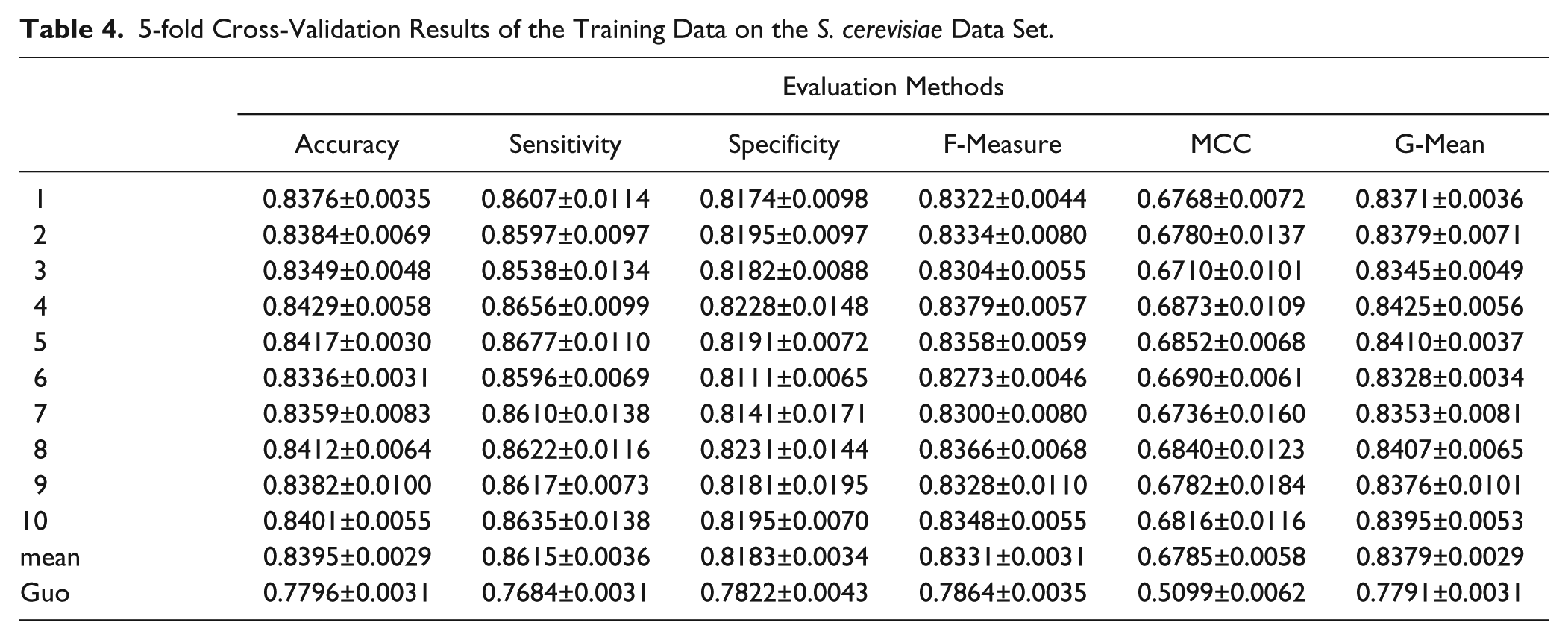
From the results shown in Table 4 , we can see that the proposed model achieves a good performance on the training data set. The average results of the model are 0.8395 for accuracy, 0.6785 for the MCC, 0.8379 for the geometric mean, 0.8331 for the F-measure, 0.8615 for sensitivity, and 0.8183 for specificity.

After the 5-fold cross-validation, the independent-test data set, the remaining pairs of the data set, was also applied to further evaluate the proposed predictors. In the test data, 11,562 positive samples and 21,261 negative samples are included. The experimental results are shown in Table 5 .

Table 5.

Performance on the Independent-Test Data of the S. cerevisiae Data Set.

	Evaluating Methods
	Accuracy	Sensitivity	Specificity	F-Measure	MCC	G-Mean
1	0.8558	0.7859	0.8958	0.7986	0.6866	0.8451
2	0.8596	0.7842	0.9043	0.8063	0.6970	0.8524
3	0.8586	0.7896	0.8981	0.8026	0.6927	0.8482
4	0.8526	0.7782	0.8960	0.7954	0.6808	0.8432
5	0.8582	0.7902	0.8969	0.8017	0.6915	0.8473
6	0.8582	0.7855	0.9007	0.8033	0.6930	0.8495
7	0.8591	0.7891	0.8994	0.8037	0.6942	0.8494
8	0.8547	0.7849	0.8945	0.7969	0.6840	0.8436
9	0.8518	0.7737	0.8983	0.7957	0.6803	0.8439
10	0.8574	0.7846	0.8998	0.8021	0.6911	0.8485
mean	0.8566±0.0026	0.7846±0.0049	0.8984±0.0027	0.8006±0.0035	0.6891±0.0055	0.8471±0.0029
Guo	0.7865±0.0030	0.6485±0.0044	0.8500±0.0034	0.7219±0.0029	0.5171±0.0048	0.7929±0.0025

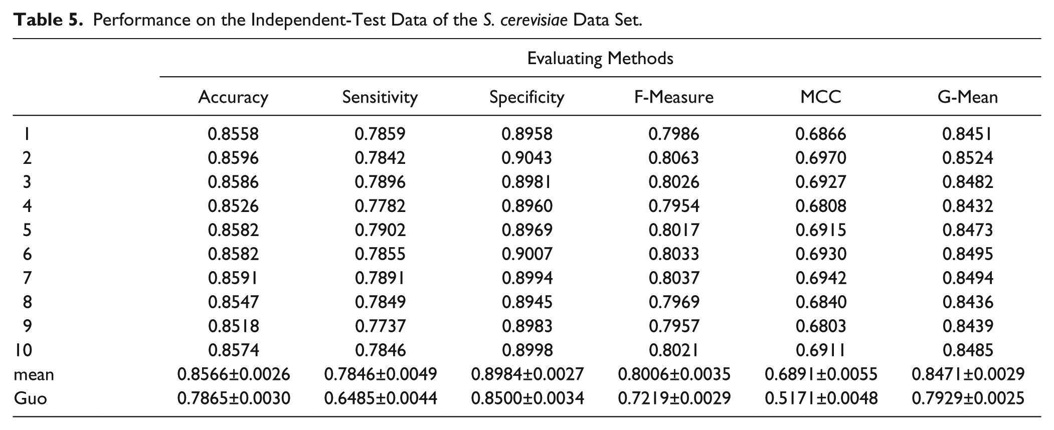
From the results shown in Table 5 , we can see that the proposed model achieves a good performance on the testing data set. The average results of the predictor on the test data set are 0.8566 for accuracy, 0.6891 for the MCC, 0.8471 for the geometric mean, 0.8006 for the F-measure, 0.7846 for sensitivity, and 0.8984 for specificity.

Compared with Other Methods

In addition, we compared the effectiveness of our proposed model with the method proposed by Guo.¹⁰ The model also used only the sequence features to predict the PPIs. The auto-covariance (AC) features and support vector machine (SVM) are used for prediction. AC accounts for the interactions between residues that are a certain distance apart in the sequence, so this model mainly takes the neighboring effect into account. The definition of AC is as follows:

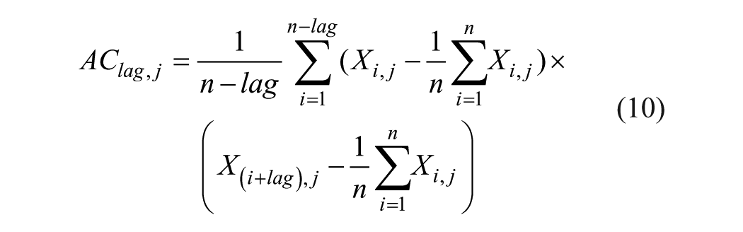
A C_{l a g, j} = \frac{1}{n - l a g} \sum_{i = 1}^{n - l a g} (X_{i, j} - \frac{1}{n} \sum_{i = 1}^{n} X_{i, j}) \times (X_{(i + l a g), j} - \frac{1}{n} \sum_{i = 1}^{n} X_{i, j})

where j represents one descriptor such as the physiochemical descriptors of the amino acids, which composed the protein; i is the position in sequence X; n is the length of sequence X; and lag is the value of the lag (the maximum distance between an amino acid residue and its neighbor with a certain number of residues away). In this work, a protein pair is converted into a 420-dimensional (2 × 30 × 7) vector by AC with a lag of 30 amino acids, where 2 is the number of two protein sequences and 7 is the number of descriptors. The experimental results on training data and testing data are shown in Figure 4 .

Figure 4.

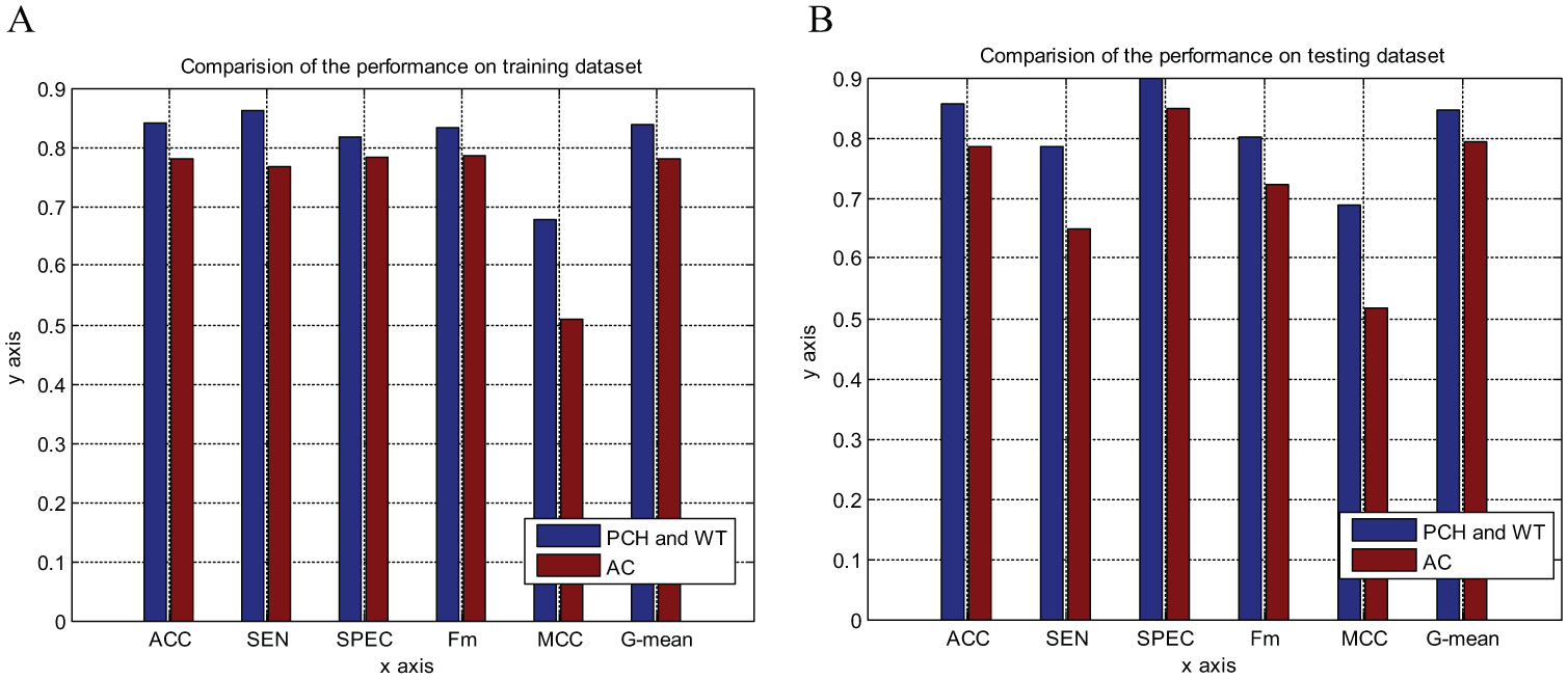
Comparison of the proposed predictor with Guo’s predictor (A) on the training data set; and (B) on the testing data set. The value shown is the mean value of 10 times.

From Figure 4 , we can see that the performance of the proposed model is better than that of the AC model, especially regarding the MCC value. This means that the proposed model has higher accuracy with both negative and positive samples, and possesses better prediction ability. Furthermore, we must point out that the number of extracted features of our model is only 280, which is less than the AC model has (with 420 features). So we use less features and computational costs, but get a better performance.

In this section, we compared the results of the proposed method with those of the existing methods on the H. pylori data set. The results of 10-fold cross-validation over several different methods^{11,21,41–44} on the H. pylori data set are shown in Table 6 . In Boch and Gough’s approach,^41,45 several structural and physiochemical descriptors with SVM as the classifier were used to predict PPIs. And, in the method of Martin et al.,²¹ a novel descriptor called a signature product was developed, which is a product of subsequence and an expansion of a signature descriptor from chemical informatics to infer PPIs. Nanni developed a PPI predictor base on a K-local hyperplane.⁴⁴ In Nanni and Lumini’s paper,⁴² they developed an ensemble of K-local hyperplanes for predicting PPIs. In another article, Nanni⁴³ designed a feature vector based on 2 g, and then input it into linear discriminant classifiers for the prediction of PPIs. Nanni and Lumini⁴² fused some hyperplane distance nearest-neighbor classifiers to identify PPIs. Xia¹¹ developed a sequenced-based predictor based on an autocorrelation descriptor and rotation forests.

Table 6.

Comparison of State-of-the-Art Methods with 10-Cross-Validation.

Methods	Sensitivity	Precision	Accuracy
Bock and Gough^a	0.698	0.802	0.758
Martin^b	0.799	0.857	0.834
Nanni^c	0.806	0.851	0.830
Nanni^d	0.860	0.840	0.840
Nanni and Lumini^e	0.867	0.850	0.866
Xia^f	0.882	0.892	0.884
Our method^g	0.867	0.910	0.887

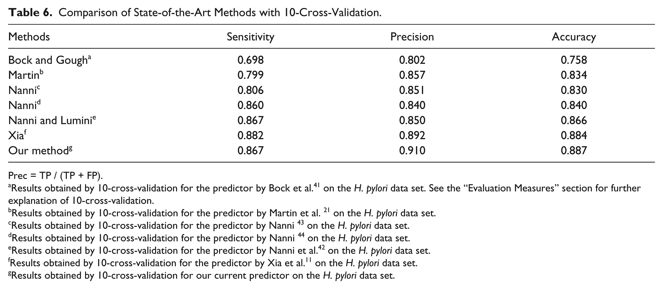
Prec = TP / (TP + FP).

Results obtained by 10-cross-validation for the predictor by Bock et al.⁴¹ on the H. pylori data set. See the “Evaluation Measures” section for further explanation of 10-cross-validation.

Results obtained by 10-cross-validation for the predictor by Martin et al. ²¹ on the H. pylori data set.

Results obtained by 10-cross-validation for the predictor by Nanni ⁴³ on the H. pylori data set.

Results obtained by 10-cross-validation for the predictor by Nanni ⁴⁴ on the H. pylori data set.

Results obtained by 10-cross-validation for the predictor by Nanni et al.⁴² on the H. pylori data set.

Results obtained by 10-cross-validation for the predictor by Xia et al.¹¹ on the H. pylori data set.

Results obtained by 10-cross-validation for our current predictor on the H. pylori data set.

We can observe that our method clearly achieves the best results for accuracy and precision compared to the other four approaches. Only the sensitivity was slightly lower than with Xia’s methods. The results for the two data sets showed that the proposed predictor was a useful supplementary tool for PPI prediction.

Conclusion

In this work, a new PPI prediction model is proposed that uses only the primary sequences of proteins. The protein features are extracted by using the physicochemical descriptor and DWT, and random forests algorithm is used for prediction. We evaluate the model on large-scale test data. The prediction results clearly show that our model is effective in PPI prediction. Furthermore, fewer features are used in the model, but better performance can be achieved. The PPI predictor is available on a public server (http://www.jci-bioinfo.cn/PPI_RF).

Footnotes

Declaration of Conflicting Interests

The authors declared no potential conflicts of interest with respect to the research, authorship, and/or publication of this article.

Funding

The authors disclosed receipt of the following financial support for the research, authorship, and/or publication of this article: This work was partially supported by the National Nature Science Foundation of China (Nos. 61261027, 61262038, 31260273, and 61202313); the Natural Science Foundation of Jiangxi Province, China (Nos. 20122BAB211033, 20122BAB201044, and 20132BAB201053); the Scientific Research Plan of the Department of Education of Jiangxi Province (GJJ14640); and the Young Teacher Development Plan of the Visiting Scholars Program, University of Jiangxi Province. The funders had no role in study design, data collection and analysis, decision to publish, or preparation of the manuscript.

References

Fields

Song

A Novel Genetic System to Detect Protein-Protein Interactions. Nature. 1989, 340, 245–246.

Ito

Chiba

Ozawa

. A Comprehensive Two-Hybrid Analysis to Explore the Yeast Protein Interactome. Proc. Natl. Acad. Sci. USA. 2001, 98, 4569–4574.

Gavin

A-C.

Bosche

Krause

. Functional Organization of the Yeast Proteome by Systematic Analysis of Protein Complexes. Nature. 2002, 415, 141–147.

Gruhler

Heilbut

. Systematic Identification of Protein Complexes in Saccharomyces cerevisiae by Mass Spectrometry. Nature. 2002, 415, 180–183.

Zhu

Bilgin

Bangham

. Global Analysis of Protein Activities Using Proteome Chips. Science. 2001, 293, 2101–2105.

Han

J-D. J.

Dupuy

Bertin

. Effect of Sampling on Topology Predictions of Protein-Protein Interaction Networks. Nat. Biotechnol. 2005, 23, 839–844.

Anfinsen

C. B.

Principles That Govern the Folding of Protein Chains. Science. 1973, 181, 223–230.

Gomez

S. M.

Noble

W.S.

Rzhetsky

Learning to Predict Protein-Protein Interactions from Protein Sequences. Bioinformatics. 2003, 19, 1875–1881.

Shen

Zhang

Luo

. Predicting Protein-Protein Interactions Based Only on Sequences Information. Proc. Natl. Acad. Sci. USA. 2007, 104, 4337–4341.

10.

Guo

Wen

. Using Support Vector Machine Combined with Auto Covariance to Predict Protein-Protein Interactions from Protein Sequences. Nucleic Acids Res. 2008, 36, 3025–3030.

11.

Xia

J-F.

Han

Huang

D-S.

Sequence-Based Prediction of Protein-Protein Interactions by Means of Rotation Forest and Autocorrelation Descriptor. Protein Pep. Lett. 2010, 17, 137–145.

12.

Xia

J-F.

Zhao

X-M.

Huang

D-S.

Predicting Protein-Protein Interactions from Protein Sequences Using Meta Predictor. Amino Acids. 2010, 39, 1595–1599.

13.

Yang

Xia

J-F.

Guim

Prediction of Protein-Protein Interactions from Protein Sequence Using Local Descriptors. Protein Pep. Lett. 2010, 17, 1085–1090.

14.

Pellegrini

Marcotte

E. M.

Thompson

M. J.

. Assigning Protein Functions by Comparative Genome Analysis: Protein Phylogenetic Profiles. Proc. Natl. Acad. Sci. USA. 1999, 96, 4285–4288.

15.

Pazos

Valencia

Similarity of Phylogenetic Trees as Indicator of Protein-Protein Interaction. Protein Eng. 2001, 14, 609–614.

16.

Overbeek

Fonstein

D’Souza

. Use of Contiguity on the Chromosome to Predict Functional Coupling. In Silico Bio. 1999, 1, 93–108.

17.

Enright

A. J.

Iliopoulos

Kyrpides

N. C.

. Protein Interaction Maps for Complete Genomes Based on Gene Fusion Events. Nature. 1999, 402, 86–90.

18.

Marcotte

E. M.

Pellegrini

H-L.

. Detecting Protein Function and Protein-Protein Interactions from Genome Sequences. Science. 1999, 285, 751–753.

19.

Huang

T-W.

Tien

A-C.

Huang

W-S.

. POINT: A Database for the Prediction of Protein-Protein Interactions Based on the Orthologous Interactome. Bioinformatics. 2004, 20, 3273–3276.

20.

Espadaler

Romero-Isart

Jackson

R. M.

. Prediction of Protein-Protein Interactions Using Distant Conservation of Sequence Patterns and Structure Relationships. Bioinformatics. 2005, 21, 3360–3368.

21.

Martin

Roe

Faulon

J-L.

Predicting Protein-Protein Interactions Using Signature Products. Bioinformatics. 2005, 21, 218–226.

22.

Chou

K-C.

Cai

Y-D.

Predicting Protein-Protein Interactions from Sequences in a Hybridization Space. J. Proteome Res. 2006, 5, 316–322.

23.

Daubechies

The Wavelet Transform, Time-Frequency Localization and Signal Analysis. IEEE T. Inform. Theory. 1990, 36, 961–1005.

24.

Breiman

Random Forests. Mach. Learn. 2001, 45, 5–32.

25.

Salwinski

Miller

C. S.

Smith

A. J.

. The Database of Interacting Proteins. Nucleic Acids Res. 2004, 32, D449–D451.

26.

Godzik

CD-HIT: A Fast Program for Clustering and Comparing Large Sets of Protein or Nucleotide Sequences. Bioinformatics. 2006, 22, 1658–1659.

27.

Ben-Hur

Noble

W. S.

Choosing Negative Examples for the Prediction of Protein-Protein Interactions. BMC Bioinformatics. 2006, 7, S2.

28.

Tanford

Contribution of Hydrophobic Interactions to the Stability of the Globular Conformation of Proteins. J. Amer. Chem. Soc. 1962, 84, 4240–4247.

29.

Hopp

T. P.

Woods

K. R.

Prediction of Protein Antigenic Determinants from Amino Acid Sequences. Proc. Natl. Acad. Sci. USA. 1981, 78, 3824–3828.

30.

Krigbaum

W. R.

Komoriya

Local Interactions as a Structure Determinant for Protein Molecules. BBA-Protein Struct. 1979, 576, 204–228.

31.

Grantham

Amino Acid Difference Formula to Help Explain Protein Evolution. Science. 1974, 185, 862–864.

32.

Charton

B. I.

The Structural Dependence of Amino Acid Hydrophobicity Parameters. J. Theor. Biol. 1982, 99, 629–644.

33.

Rose

G. D.

Geselowitz

A. R.

Lesser

G. J.

. Hydrophobicity of Amino Acid Residues in Globular Proteins. Science. 1985, 229, 834–838.

34.

Zhou

Tian

. Genetic Algorithm-Based Virtual Screening of Combinative Mode for Peptide/Protein. Acta Chim. Sinica. 2006, 64, 691–697.

35.

Mallat

S. G.

A Theory for Multiresolution Signal Decomposition: The Wavelet Representation. IEEE T. Pattern Anal. 1989, 11, 674–693.

36.

Mallat

A Wavelet Tour of Signal Processing. Academic Press: New York, 1999.

37.

Qiu

J-D.

Sun

X-Y.

Suo

S-B.

. Predicting Homo-Oligomers and Hetero-Oligomers by Pseudo-Amino Acid Composition: An Approach from Discrete Wavelet Transfor-mation. Biochimie. 2011, 93, 1132–1138.

38.

Mitchell

T. M.

Machine Learning. McGraw Hill: New York, 1997.

39.

Matthews

B. W.

Comparison of the Predicted and Observed Secondary Structure of T4 Phage Lysozyme. BBA-Protein Struct. 1975, 405, 442–451.

40.

Jia

Xiao

Liu

. Bagging-Based Spectral Clustering Ensemble Selection. Pattern. Recogn. Lett. 2011, 32, 1456–1467.

41.

Bock

J. R.

Gough

D. A.

Whole-Proteome Interaction Mining. Bioinformatics. 2003, 19, 125–134.

42.

Nanni

Lumini

An Ensemble of K-Local Hyperplanes for Predicting Protein-Protein Interactions. Bioinformatics. 2006, 22, 1207–1210.

43.

Nanni

Fusion of Classifiers for Predicting Protein-Protein Interactions. Neurocomputing. 2005, 68, 289–296.

44.

Nanni

Hyperplanes for Predicting Protein-Protein Interactions. Neurocomputing. 2005, 69, 257–263.

45.

Bock

J. R.

Gough

D. A.

Predicting Protein-Protein Interactions from Primary Structure. Bioinformatics. 2001, 17, 455–460.

Prediction of Protein–Protein Interactions with Physicochemical Descriptors and Wavelet Transform via Random Forests

Abstract

Keywords

Introduction

Materials and Methods

Data Collection and Data Set Construction

Feature Extraction

Random Forests Algorithm

Evaluation Measures

Web Server and User Guide

Results and Discussion

Effect of Wavelet Functions

Performance on the S. cerevisiae Data Set

Compared with Other Methods

Conclusion

Footnotes

Declaration of Conflicting Interests

Funding

References