
Abstract
A scheduler has been developed for an integrated laboratory robot system that operates in an always-on mode. The integrated system is designed for imaging plates containing protein crystallization experiments, and it allows crystallographers to enter plates at any time and request that they be imaged at multiple time points in the future. The scheduler must rearrange tasks within the time it takes to image one plate, trading off the quality of the schedule for the speed of the computation. For this reason, the scheduler was based on a simulated annealing algorithm with an objective function that makes use of a linear programming solver. To optimize the scheduler, extensive computational simulations were performed involving a difficult but representative scheduling problem. The simulations explore multiple configurations of the simulated annealing algorithm, including both geometric and adaptive annealing schedules, 3 neighborhood functions, and 20 neighborhood diameters. An optimal configuration was found that produced the best results in less than 60 seconds, well within the window necessary to dynamically reschedule imaging tasks as new plates are entered into the system.
Introduction
An automated system has been developed that performs periodic imaging of hanging-drop and sitting-drop vapor diffusion experiments for protein crystallization. All experiments are set up in commercially available 96-well protein crystallization plates containing one to three drops per well. The number of drops in an individual plate is determined by the plate geometry as well as the goals of the crystallization experiment. All drops in a given plate are imaged during a single imaging event.
The automated system integrates a variety of devices, including a robotic arm for plate transfer, one automated digital microscope for image capture, and plate storage. (See Figure 1 .) The system operates in an always-on mode, allowing crystallographers to introduce new experiment plates at any time and to request that they be imaged at multiple time points in the future. When a plate is due to be imaged, the robot automatically retrieves it from storage and delivers it to the digital microscope, where detailed images of all drops are collected at multiple focal depths. Images are saved and analyzed before the robot returns the plate to storage. The imaging duration of a single plate typically varies between 20 and 40 minutes depending on the number of drops set up in the plate and the amount of processing required to locate each drop and collect images at multiple focal depths.
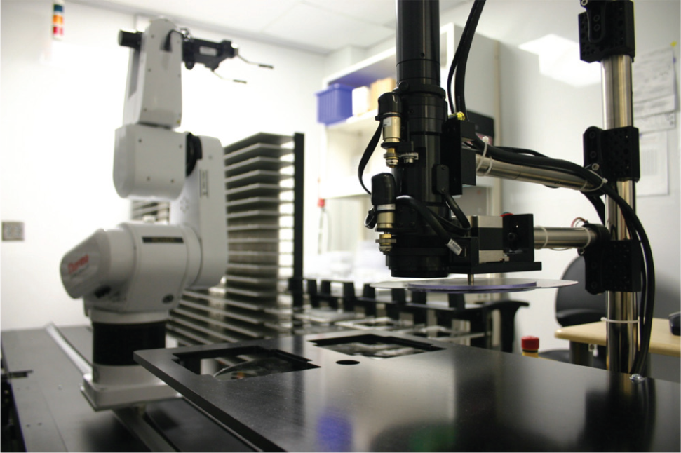
A view of the integrated system, showing the automated imager in the foreground, the articulated robot arm on the left, and plate storage in the background.
The automated digital microscope is able to image the drops of one plate at a time. Because the crystallographers may add plates to the system at will and request that they be imaged at multiple future times, it is common for scheduling conflicts to occur. This requires the tasks on the master imaging schedule to be rearranged on the fly in an attempt to better achieve the timing goals of all experiments.
Plate-imaging tasks are assigned a priority. As a general rule, the longer that a plate remains in the system, the lower the priority of its next imaging task. Task priority is taken into account when two or more imaging tasks are in conflict. A scheduling algorithm was developed that automatically adjusts the requested times for imaging tasks in an attempt to optimize the order on a master schedule. One task order is preferred over another if imaging tasks with a higher priority occur more closely to their requested absolute time as compared with imaging tasks with a lower priority. It is important to note that the scheduling algorithm presented here is useful for approximating the optimal schedule for any system in which tasks of varying priority involving a single shared resource are requested to occur at potentially conflicting future time points.
A key requirement of the scheduling algorithm is that it must produce reasonable task schedules within the time it takes to image one plate, which can be as little as 20 minutes. The size of the problem (40 to 50 tasks in a 24-hour period of time was common) makes computing a guaranteed optimal schedule prohibitively expensive. Fortunately, an optimal schedule is not necessary; a schedule that comes reasonably close to an optimum is sufficient. For this reason, we investigated simulated annealing1,2,3 as the primary computational technique for the scheduler.
Numerous previous investigations have explored the use of simulated annealing as a technique for solving scheduling problems, including one similar to ours called the job shop scheduling problem; for example, see van Laarhoven et al. (1992). 4 A job shop consists of a finite set of machines on which a number of jobs are to be performed. Each job involves visiting a subset of the machines in a specific predefined order. The machines and the order in which they are visited can be different for each job. Once a job is on a machine, it cannot be interrupted, and each machine can process only one job at a time. The amount of machine time each job must use also may vary. The problem is to find a master task schedule that instructs all jobs to visit necessary machines in the prespecified order for the required amount of time such that the overall makespan is minimized. Makespan is defined as the total duration between the start of the first task and the end of the last task of a given schedule.
Our scheduling problem is similar in spirit but different in several important ways. For example, the only machine in our integrated system that is considered by the scheduler is the imager. The time required to process plates on other machines is negligible by comparison and therefore ignored. Perhaps the most important difference between scheduling a job shop and our problem is that tasks to be scheduled have been assigned absolute start times as well as execution priorities. The absolute times at which tasks in a job shop begin as well as their relative priorities are not important; it is important only that they occur in the specified order. Our scheduler must look ahead for periods when the imager is oversubscribed and minimize the negative impact of this bottleneck. The scheduler must perform this function repeatedly while the system is in continuous operation for extended durations (e.g., months) and as plates are added to or removed from the system.
A representative scheduling problem was formulated and used as a tool to find a reasonable set of parameters with which to perform scheduling in the current environment using simulated annealing. This problem captures one of the more challenging task arrangements to be scheduled among all possible variations. Both deterministic and adaptive annealing schedules are investigated, as are multiple neighborhood functions used to reorder tasks after each simulated annealing trial. A formulation of the objective function used for the simulated annealing algorithm is presented, which is based on linear programming. 5 This is followed by a description of the analysis that was performed and the results obtained that suggest the best method for approximating the optimal plate-imaging task schedule.
Materials and Methods
A Representative Scheduling Problem
In practice, the actual number of plate-imaging tasks scheduled for a given period of time can vary widely. The number of plates in the system at any moment depends on the current demand for protein crystal structures and how readily proteins under study produce crystals suitable for X-ray diffraction. To develop and tune our scheduling algorithm, we defined a representative scheduling problem that exhibits challenging but typical scheduling conflicts observed in practice.
Our representative scheduling problem is made up of 50 plate-imaging tasks that are requested to occur at times organized as five groups of 10. Each imaging task is assumed to require 20 minutes for plate transfer and image capture of all drops. The tasks within each group of 10 are initially requested to occur at exactly the same time, meaning that all 10 tasks are in conflict. Each task within a group of 10 is assigned a different priority value, from 1 to 10. The five task groups are separated by one-hour intervals. Because our timeline is considered infinite in both directions, the clock time for each group is not important, only the number of tasks and relative spacing. Nevertheless, for convenience, we assume that tasks within groups are set to begin at 10:00 a.m. (600 minutes), 11:00 a.m. (660 minutes), 12:00 p.m. (720 minutes), 1:00 p.m. (780 minutes), and 2:00 p.m. (840 minutes).
An illustration of the representative scheduling problem is depicted in Figure 2 . Each task is represented as a block, in which the width of the block is proportional to the duration of the task (20 minutes). Blocks are stacked on top of one another when they are in conflict. Consequently, Figure 2 depicts five groups of 10 tasks as five stacks of 10 blocks in which all of the tasks within a group are in conflict. Task blocks are labeled with task number, ranging from 1 through 50. Blocks in each stack have priorities from 1 to 10, as indicated by the notation on the left side of the diagram. The scheduling problem can be thought of as spreading out all 50 blocks on the timeline so that none are stacked and those with a higher priority are positioned closer to their desired start time. Note that at 20 minutes per plate, a stack of 10 plates would require 200 minutes to complete. But each stack is separated by only 60 minutes. The scheduling algorithm will be forced to interleave the tasks of different groups to obtain a good schedule.
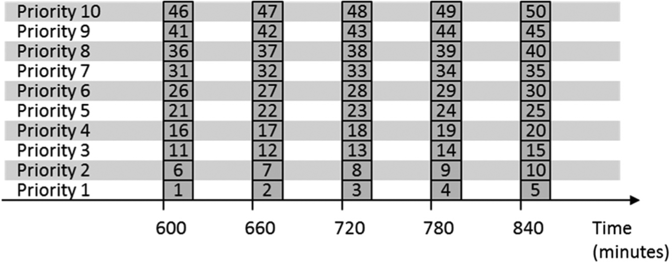
An illustration of the representative scheduling problem used to explore the simulated annealing scheduling algorithm.
Problem Formulation
The following parameter definitions are used throughout the formulation of the problem, including the objective function and the scheduling algorithm itself.
We divide the overall scheduling problem into two subproblems. Informally, we refer to these as the shifting problem and the ordering problem. The shifting problem starts with a given fixed order for all tasks, but no scheduled start times. The shifting problem solver shifts all tasks along the master timeline to compute a scheduled start time for each task that minimizes some objective function. Each task can be shifted individually as necessary, but the relative task order cannot be modified. An ordering problem solver complements the shifting problem solver in that it reorders tasks in an attempt to find the overall best task execution order.
A complete task scheduler combines solvers for both the ordering problem and the shifting problem. The scheduler starts by selecting an initial task order. Then, given this order, the shifting problem solver schedules start times for all tasks that minimize an objective function. The final value of the shifting problem’s objective function also is used as the overall objective function value for that particular solution. The ordering problem solver generates a new task order, which is shifted once again using the shifting problem solver to produce a new objective function value. The new task order is either accepted or rejected based on how the new objective function value compares with the old value. This iterative process—alternately applying each solver—repeats until a suitable stopping condition is satisfied. Stated in terms of the parameter definitions listed in Table 1 , the ti values are modified during the iterative scheduling process in an effort to lower the value of OT, subject to the constraint that no two tasks may conflict by overlapping in time.
Parameter Definitions.
Shifting Problem
The objective function used by the shifting problem solver and to compare task schedules is computed as a weighed sum of the absolute value of the difference between a task’s scheduled start time and its requested start time (equation 1).

The weighting parameters (wi) are used to indicate the relative priority of each task. A higher wi value causes a task to have a higher relative priority by increasing the amount contributed (Oi) to the total objective function (OT). Weights are assigned values based on the order in which a plate’s tasks are executed; the first imaging task for a given plate is assigned the largest weight, and subsequent tasks are assigned decreasing weights. Requested start times (si) are assigned by the scientist as plates are entered into the system. The scheduled start time for a plate’s imaging tasks (ti) is determined by the solver. The total objective function value (OT) for an entire task schedule is then computed as a weighted sum over all tasks (equation 1).
A linear programming solver 5 is used to compute an optimal solution to the shifting problem. Input to the linear programming solver includes the objective function to be minimized as well as a set of inequalities (equation 2) that must be satisfied by adjusting its parameters (ti). This set of inequalities expresses all constraints necessary to enforce a given task order. For example, the ith task can start no earlier than the start time of the (i−1)th task (ti−1) plus its task duration (di−1). This leads to the set of inequalities of equation 2 for all pairs of tasks (i, i−1). For our representative scheduling problem, this includes tasks where i = 2 through i = 50, for 49 inequalities in total.

Linear programming solvers do not permit the use of an absolute value in an objective function, as is the case in equation 1. To address this issue, we use a standard trick of adding a pair of new inequalities (equation 3) to the problem for each objective function term (Oi). Each pair of inequalities forms a V-shaped region whose minimum value of 0 is centered at the task’s requested start time, when ti = si. Modifying the value of ti in either direction away from si results in an increasing contribution to the objective function. Because the two inequalities taken together require that the value of Oi be greater than both inequalities, Oi will never take a value lower than 0. An attempt to minimize this term will drive the scheduled start time toward the requested start time.
For our representative scheduling problem, the objective function in equation 1 simplifies to equation 4, and equation 3 adds an additional 100 inequalities to the total given in equation 2.


With these details in place, a linear programming problem can be formulated using the data for a specific task sequence. This includes 49 inequalities that enforce task order (equation 2), 100 additional equalities for all objective function terms (equation 3), and the objective function itself (equation 4). The shifting problem can be solved in a deterministic manner to obtain an optimal scheduled start time for each task in a given task sequence.
Ordering Problem
With the shifting problem formulated, we turn our attention to the ordering problem, which we solve using simulated annealing. 1 Simulated annealing is an optimization algorithm designed to search for the global optimum (minimum or maximum) of a complex function among potentially multiple local optima. It is particularly useful when the search space is both large and discrete, as is the case with our representative scheduling problem that has a search space of size 50!, the number of all possible orderings of 50 tasks. Simulated annealing is probabilistic in nature and therefore cannot guarantee finding of the optimum solution. For a guarantee, an exhaustive search through the entire search space would be necessary, requiring a prohibitively large amount of compute time. Simulated annealing has been shown to perform well at locating near-optimal solutions when a limited amount of compute time is available.
The simulated annealing algorithm draws inspiration from the physical act of annealing metals, which involves a slow cooling process that maximizes internal atomic order and therefore minimizes thermodynamic free energy. Using this analogy, the objective function to be minimized with simulated annealing is a proxy for the thermodynamic free energy. The way in which temperature changes during the cooling process, referred to as the annealing schedule, is one of the primary factors that governs the amount of compute time necessary and the quality of the computed result.
As mentioned, the state space of the ordering problem is represented by all possible task orderings on the timeline. Modifying the task order explores the state space in an attempt to locate minima of the objective function. The method by which task order changes during each iteration of simulated annealing is called the neighborhood function because the task rearrangement is limited to a randomly selected contiguous subset of tasks (neighborhood).
After the annealing schedule, the neighborhood function is the second factor considered that governs the behavior of our simulated annealing algorithm. We tested three variations on the neighborhood function to find the best approach for solving the scheduling problem; these are described in more detail later. The third factor considered is the neighborhood diameter, which specifies the size of the neighborhood within which the neighborhood function operates. It can be as wide as the entire 50-task span, or as small as two adjacent tasks.
Each iteration of simulated annealing ends with a newly proposed task schedule, which is either accepted or rejected. If accepted, the new task order is used as input to the next iteration. If rejected, the previous task order is restored prior to the next iteration. The decision to accept or reject a proposed task order is based on a computed probability (P). If a new task order (at iteration j) results in an objective function value (OT,j) that is less than the previous iteration’s objective function value (OT,j−1), then the new order is accepted with probability P = 1.0. If the new task order results in a higher objective function value, then the new order is accepted with a probability in the range of 0.0–1.0, which is a function of the current temperature (Tj), as defined by equation 5. As the annealing schedule progresses and temperature decreases, so does the probability of accepting a newly proposed task order that increases the objective function.

One iteration of the simulated annealing algorithm is outlined as follows. Iterations continue until a suitable stopping condition is satisfied.
A task is selected randomly from the current working task list.
The neighborhood function is used to change the order of tasks within the neighborhood surrounding the selected task, the size of which is specified by the neighborhood diameter.
Tasks in the new order are shifted on the timeline (i.e., the shifting problem is solved) so as to minimize the objective function.
If the new task order decreases the objective function, the new order is retained and used as input to the next iteration (P = 1.0).
If the new order increases the objective function, it is probabilistically accepted as input to the next iteration, based on the probability (P) computed using equation 5.
Annealing Schedules
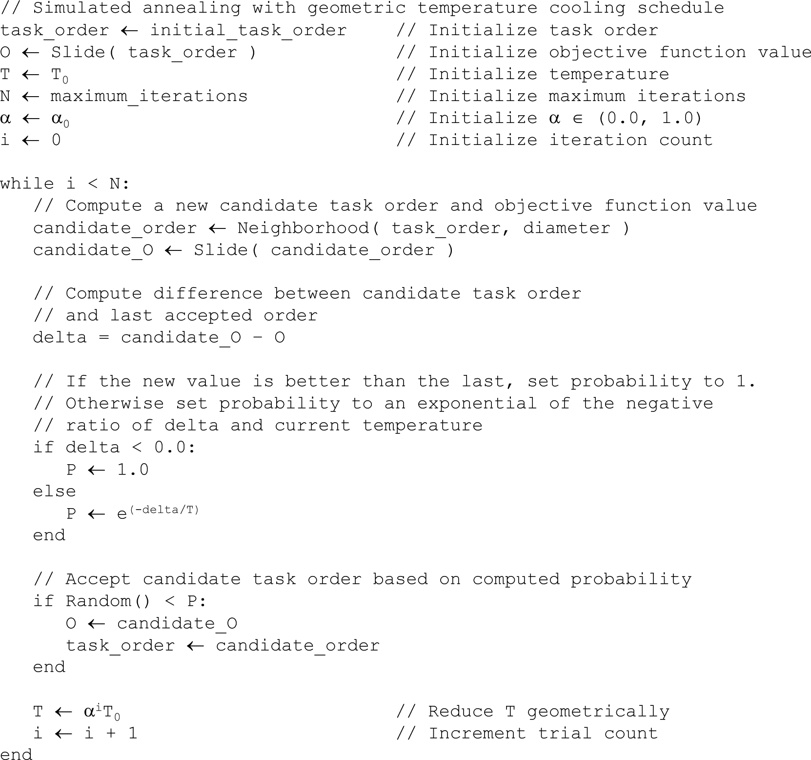
The first annealing schedule considered is called geometric cooling. In this case, temperature is initialized to some high value (T0), and it is reduced on each iteration (j) by multiplying temperature by a factor (α) that is less than 1.0 (equation 6).

Geometric cooling schedules are deterministic in the sense that temperature for any iteration is computed solely using T0, α, and the iteration number j. All of our simulations that make use of geometric cooling terminate when the temperature falls below a predetermined cutoff value.
By contrast, the second annealing schedule that we explored is referred to as Swartz’s modified Lam annealing, which was first presented by Lam and Delosme 6 and later modified by Swartz. 7 Swartz discovered that all successful annealing runs using the Lam annealing schedule shared a common pattern. He observed that the ratio of accepted to rejected moves (the accept ratio) as a function of the annealing schedule’s percentage complete followed the profile shown in Figure 3 . The accept ratio starts at 1.0 and exponentially decreases to 0.44 at a point 15% of the way through a schedule. The accept ratio remains at 0.44 until approximately 65% of the way through the schedule, at which point it resumes its exponential decline until the annealing schedule is complete at 100%. To force the accept ratio to match the profile of Figure 3 , the accept ratio is estimated continuously throughout a simulated annealing run, and the temperature is raised or lowered as necessary to force it to match the observed profile. To compare the adaptive annealing schedule with geometric cooling in a fair manner, the total number of iterations in a modified Lam annealing trial always exactly matched the total number in a trial that used geometric cooling. Later, we present the complete algorithms that implement simulated annealing with geometric cooling and the adaptive modified Lam annealing.
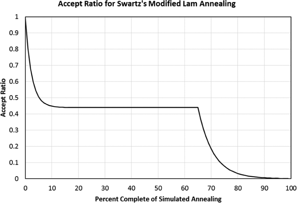
Accept rate as a function of percentage complete in Swartz’s modified Lam annealing schedule.
Neighborhood Functions and Neighborhood Diameters
Three neighborhood functions were tested, each with diameters from 1 to 20. The first neighborhood function performs an unweighted swap of two tasks. This function starts by selecting one task at random from a task schedule using a uniform random number generator. It then continues by selecting a second task at random that is separated from the first task by no more than a number of tasks defined by the diameter parameter. The second task is also selected using a uniform number generator. The positions of these two tasks are swapped in the overall task order to form a newly proposed task order. We call this neighborhood function unweighted-swap.
The second neighborhood function closely follows the procedure defined by the first, with one modification: Rather than selecting the first task in a uniformly random manner, tasks that contribute more to the overall objective function value (OT) are selected more frequently in an amount that is proportionate to their relative contribution (Oi). In other words, the likelihood that a task will be selected as the first task for a swap is weighted by the task’s contribution to the objective function. Selection of the second task follows the same technique used by the first neighborhood function, once again using diameter as a parameter to limit candidate tasks. We call this neighborhood function weighted-swap.
The third neighborhood function uses the same weighting scheme described in the second neighborhood function to select the first and second tasks; although in this case, instead of swapping the first task with the second, the first task is inserted before the second task and all tasks in between are shifted by one. We call this neighborhood function weighted-insert.
Algorithms
Algorithms for simulated annealing with geometric cooling and modified Lam annealing are presented in Figures 4 and 5 , respectively. Note that the function named slide takes a task ordering as a parameter, determines the optimum start time for all tasks using the shifting problem solver, and returns the resulting optimized objective function value. The function named neighborhood takes both a task ordering and a diameter as parameters, computes a new task order using a neighborhood function, and returns the new task order. Finally, the function named random generates a uniform random variate in the range of 0.0–1.0.
Simulated annealing algorithm using geometric cooling.
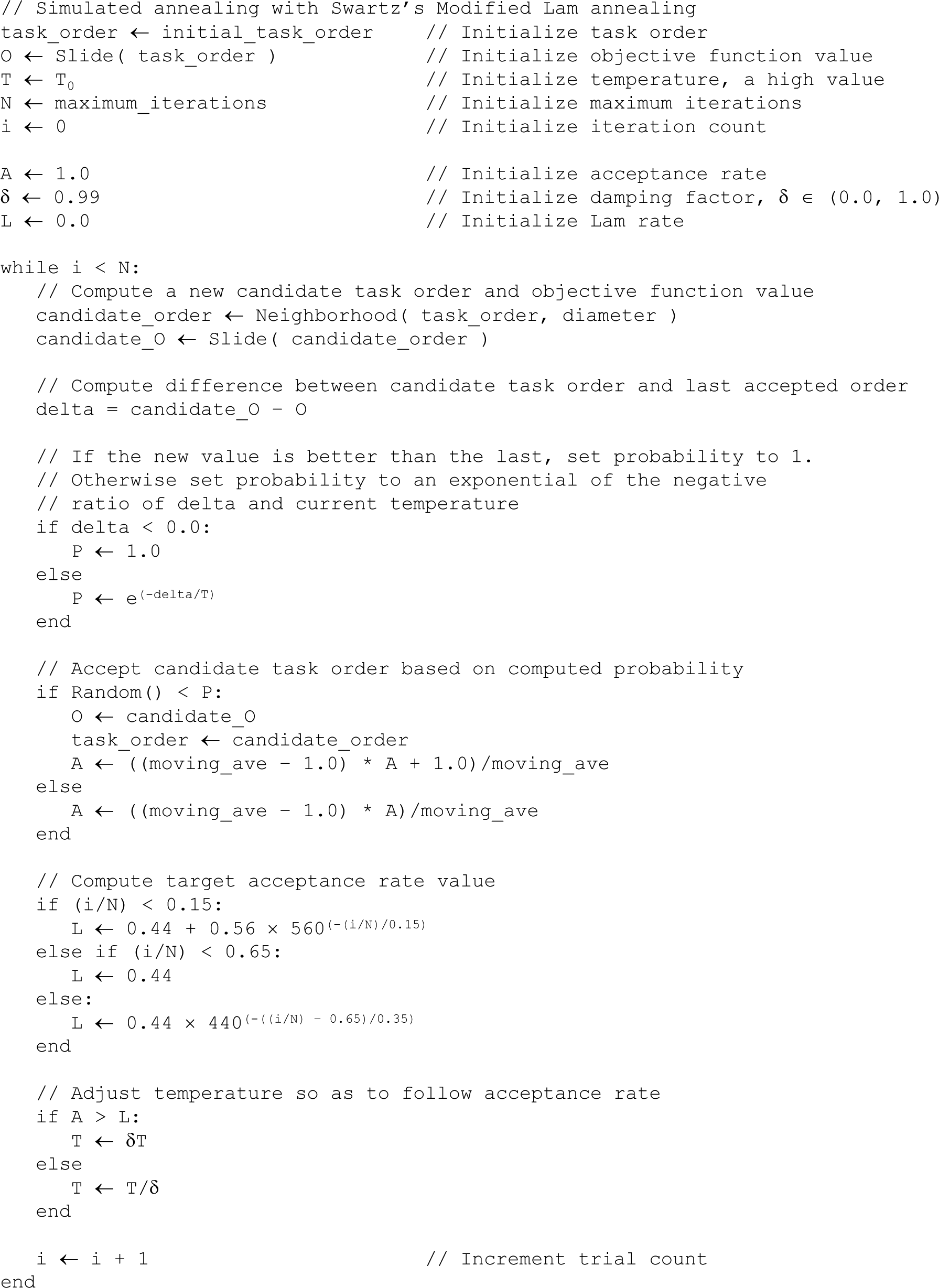
Simulated annealing algorithm using Swartz’s modified Lam annealing.
Simulations Performed
A series of computational simulations was performed in an effort to find the combination of annealing schedule, neighborhood function, and diameter that most often computes the best relative solution to the representative 50-task scheduling problem. All simulations were performed on a 64-bit, 4-core computer with 4 GB of memory running Windows 7. All individual runs completed in 55 to 56 seconds, much quicker than the 20-minute maximum.
Geometric cooling and modified Lam annealing were tested with each of the three neighborhood functions and each neighborhood diameter in the range of 1–20. All geometric cooling schedules began with T0 = 10.0, an α = 0.999, and a stopping condition of T = 1.0. This led to approximately 2300 maximum iterations in total. To ensure a fair comparison between the two annealing schedules, all modified Lam annealing runs were also constrained to 2300 maximum iterations. A simulated annealing simulation for each set of conditions was repeated 50 times, and the lowest objective function value was recorded, as was the associated final task schedule.
Results
Averages and standard deviations for the 50 repetitions of each simulation are given in Table 2 and Table 3 . Each row in the table represents a different diameter, and each column a pairing of annealing schedule and neighborhood function. All results are plotted in Figure 6 .
Average Minimum Objective Function Values for 50 Repetitions of Simulated Annealing Using the Indicated Annealing Function, Neighborhood Function, and Neighborhood Diameter.
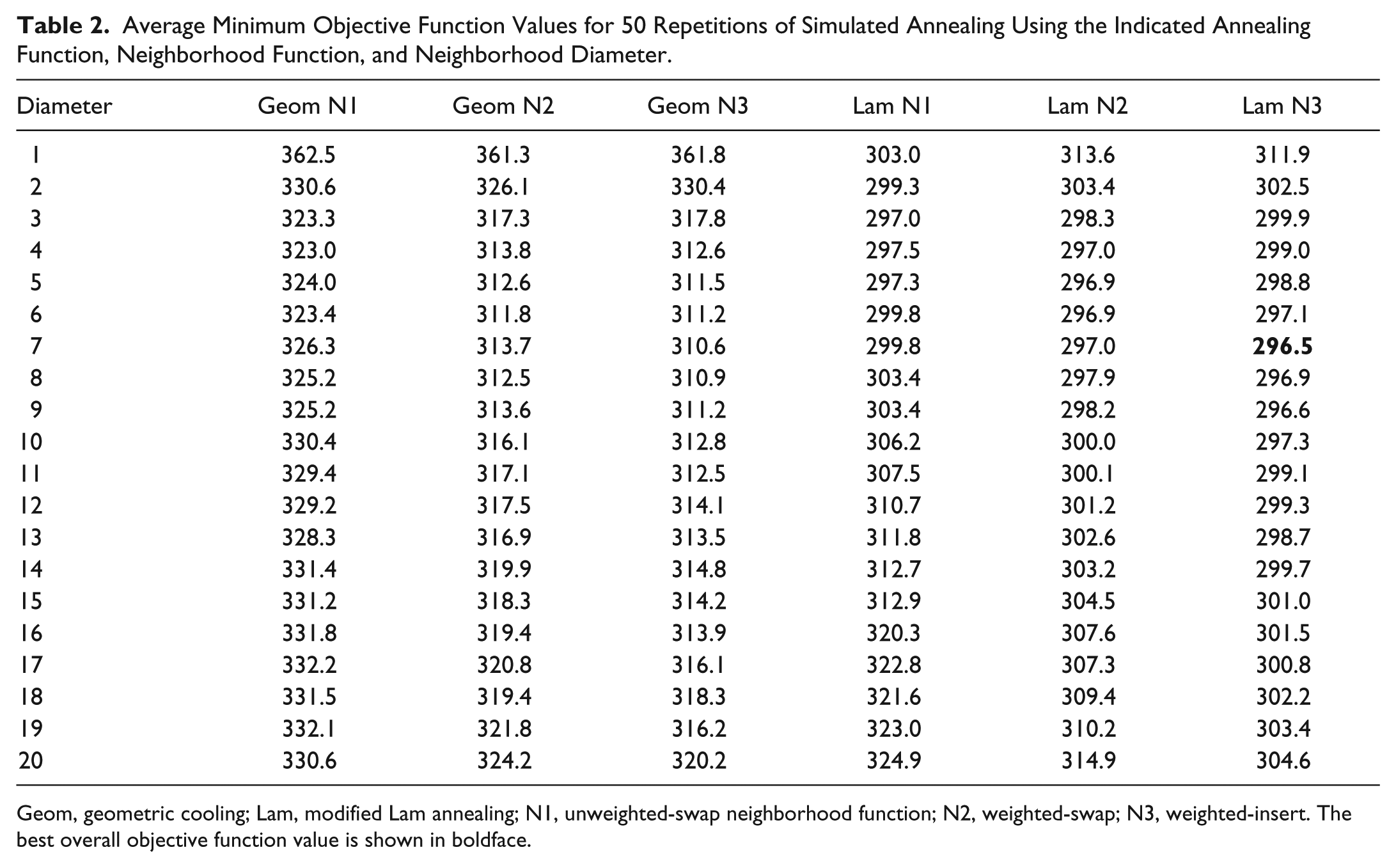
Geom, geometric cooling; Lam, modified Lam annealing; N1, unweighted-swap neighborhood function; N2, weighted-swap; N3, weighted-insert. The best overall objective function value is shown in boldface.
Standard Deviation of Minimum Objective Function Values for 50 Repetitions of Simulated Annealing Using the Indicated Annealing Function, Neighborhood Function, and Neighborhood Diameter.
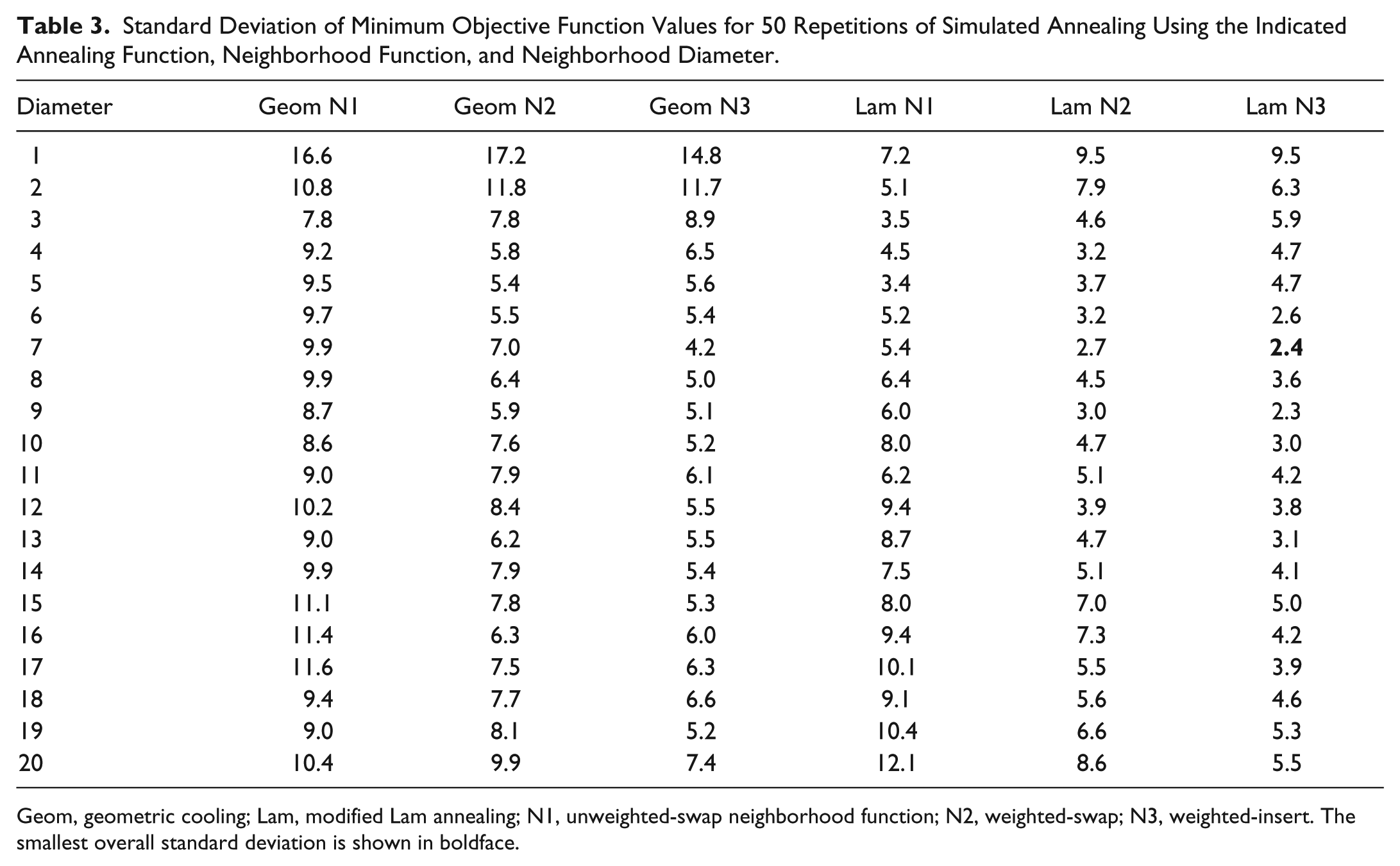
Geom, geometric cooling; Lam, modified Lam annealing; N1, unweighted-swap neighborhood function; N2, weighted-swap; N3, weighted-insert. The smallest overall standard deviation is shown in boldface.
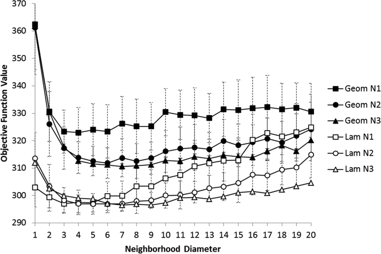
Results from all computational simulations. Geom, geometric cooling; Lam, modified Lam annealing; N1, unweighted-swap neighborhood function; N2, weighted-swap; N3, weighted-insert.
Average objective function values from the adaptive modified Lam annealing schedule were lower than those from the deterministic geometric cooling for almost all diameters. It is interesting to see that each series of simulations revealed an optimal diameter in the range of 3–7. The overall best average objective function value for the weighted-insert neighborhood function (N3) was lower than unweighted-swap (N1) and weighted-swap (N2), both occurring at a diameter of 7 for geometric cooling and modified Lam annealing. The standard deviation of these two statistics also was lowest within subsets limited to a common annealing approach. A two-sample t-test assuming unequal variances performed on these two statistics demonstrates that it is highly likely that they are significantly different, leading to the conclusion that our scheduler performs best using Swartz’s modified Lam annealing and a weighted-insert neighborhood function with a neighborhood diameter value of 7.
Figure 7 illustrates the initial schedule produced by placing all tasks on the timeline in numeric order and solving the shifting problem once, prior to any simulated annealing. The x-axis is the time at which each task will begin, and the y-axis is the amount that each task contributes to the overall objective function. Chart markers are labeled with task number, and the overall objective function value is 484.4.
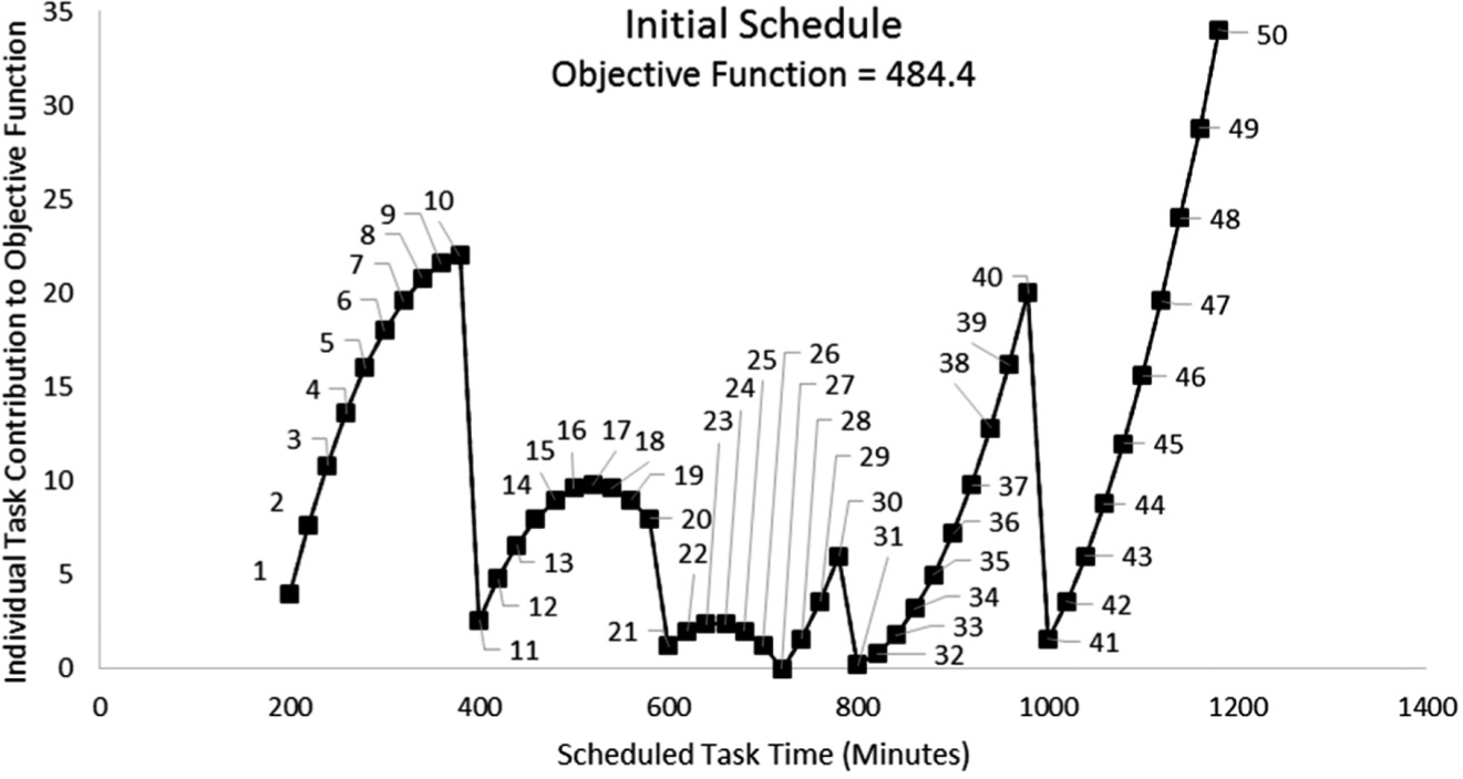
The initial schedule produced for the representative scheduling problem by placing all tasks on the timeline and solving the shifting problem once, prior to performing simulated annealing. Each marker represents a single task on the schedule, as indicated by the label. The x-axis is the task start time, and the y-axis the amount that is contributed to the objective function by each task. The starting total objective function value is 484.4.
Figure 8 illustrates an example of an optimized schedule after simulated annealing is run once using modified Lam annealing with a weighted-swap neighborhood function on a neighborhood of diameter 7. For this example, the final overall objective function value has been reduced to 294.0. Once again, the chart markers are labeled with the associated task number. One can observe how all tasks have been reordered and shifted to produce the improved schedule.
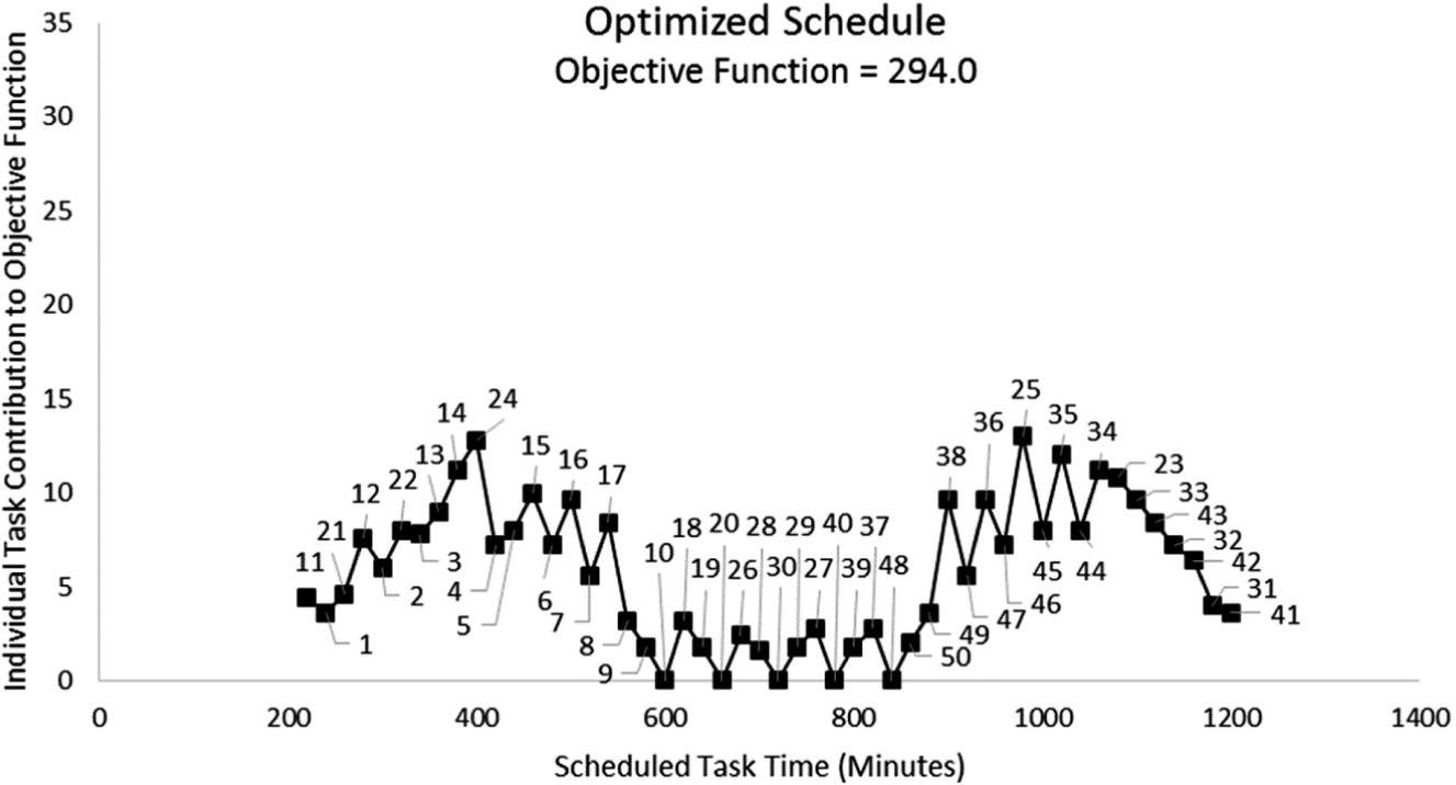
An example of one optimized schedule produced after the application of one round of simulated annealing to the representative scheduling problem. Modified Lam annealing was used with a weighted-swap neighborhood function on a neighborhood of diameter 7. The final objective function value for this example was 294.0.
Conclusion
A scheduling algorithm based on simulated annealing and linear programming was designed to optimize the order of imaging tasks to be performed by an integrated laboratory robot system built to automate protein crystallization experiments. To find the best configuration for the simulated annealing scheduler, several alternatives were investigated. Annealing schedules tested include the deterministic geometric cooling and the adaptive Swartz’s modified Lam annealing. Unweighted-swap, weighted-swap, and weighted-insert neighborhood functions were tested with each annealing schedule and neighborhood diameters from 1 to 20. A representative scheduling problem was used to explore the performance of all configurations. The problem consisted of five groups of 10 tasks, with each task having a duration of 20 minutes. The tasks within each group were assigned identical start times, and each group was spaced at 60-minute intervals, resulting in significant task scheduling conflict. A series of computational simulations was performed to find the best configuration for the scheduling algorithm. Each configuration was repeated 50 times. The best relative results were found when using the adaptive Swartz’s modified Lam annealing and the weighted-insert neighborhood function with a neighborhood diameter of 7. All individual simulations completed in 55 to 56 seconds, much quicker than the minimum plate-imaging duration of 20 minutes. The simulated annealing scheduling algorithm described here has been used for several years to schedule tasks on an integrated laboratory robot system that performs crystallization plate imaging. It has consistently produced good results throughout its lifetime.
Footnotes
Declaration of Conflicting Interests
The authors declared no potential conflicts of interest with respect to the research, authorship, and/or publication of this article.
Funding
The authors received no financial support for the research, authorship, and/or publication of this article.