Sage Journals: Discover world-class research

Abstract

A systematic method for assembling and solving complex compound distribution problems is presented in detail. The method is based on a model problem that enumerates the mathematical equations and constraints describing a source container, liquid handler, and three types of destination containers involved in a set of compound distributions. One source container and one liquid handler are permitted in any given problem formulation, although any number of compound distributions may be specified. The relative importance of all distributions is expressed by assigning weights, which are factored into the final mathematical problem specification. A computer program was created that automatically assembles and solves a complete compound distribution problem given the parameters that describe the source container, liquid handler, and any number and type of compound distributions. Business rules are accommodated by adjusting weighting factors assigned to each distribution. An example problem, presented and explored in detail, demonstrates complex and nonintuitive solution behavior.

Keywords

high-throughput chemistry informatics and software chemistry informatics

Introduction

After completing the synthesis and purification of novel compounds, many small-molecule drug discovery efforts proceed with panels of tests that determine whether compounds show sufficient promise to warrant further investigation. Tests performed can be quite diverse, looking for both activity and selectivity of a compound against a target as well as a desirable safety profile.¹ Screening techniques are always improving, reflecting advances in both the relevant science and the technology. For example, improvements in assay sensitivity reduce compound amount requirements, thereby allowing higher density microplates to be used and more compounds to be dispensed within the limited space made available by the standard footprint.

Each of the variety of assays to be performed on a novel compound imposes its own constraints on the way the compound is to be dispensed. One assay may require that a minimum amount of compound be provided, whereas another may require an exact amount. An assay may require that the compound being tested be dissolved to a predetermined concentration or to a concentration value within a range. If target amounts or concentrations cannot be achieved, it may not be feasible to perform an assay or subsequent assays. Containers chosen place constraints on what is feasible. For example, the physical size of a source container places inherent limits on dilution volumes. The same is true for destination containers. Liquid-handling devices impose constraints, such as the volume that can be transferred and the amount of dead volume that is physically inaccessible. As the number and diversity of assay formats expand, so does the complexity of planning a procedure for creating all desired distributions from a single source container. Finding an optimal procedure for diluting and pipetting a compound from its source to various destination containers can be a tedious trial-and-error process and may in fact be impossible due to subtle conflicting constraints.

In this article, we describe a computational method that builds upon earlier work.² The method automatically computes the optimal method for performing compound distributions such as those just described. Steps of the method include (1) specifying all distributions and container types that are involved in a distribution problem, (2) identifying all conditions that must be satisfied as a set of parameterized mathematical constraints, (3) assembling all constraints involved as a mathematical problem statement in a suitable format, and (4) executing the appropriate numerical solution technique to solve for optimal transfer and dilution volumes. We will lay out the mathematical details for the class of problems that fall within our model and describe how to automate the assembly of these details into a suitable mathematical statement that can be solved automatically. We close by investigating a representative example that demonstrates the potential complexity of solutions generated.

Model Problem

Compound distribution problems can vary considerably and must be considered on a case-by-case basis. In this section, we describe in detail our general model for a compound distribution. The model is readily extended to account for other scenarios.

We assume that the compound to be distributed starts in a single source container. The source container is first diluted, and all distributions are aspirated and dispensed into one or more destination containers. One transfer from the source to a destination is called a distribution. It is possible to mark a distribution as being required or optional. We assume that the compound in the source container starts out dry, although our solution technique is easily extended to allow source compound containers to start dissolved in a known volume of solvent. All container types used have intrinsic minimum and maximum volumes that must be satisfied when attempting to compute a solution. For example, a source container can never be diluted beyond its maximum volume. Likewise, the volume of dissolved compound transferred to a destination container must be no less than its minimum container volume, and the sum of the transfer and dilution volumes pipetted into a destination container must be no greater than its maximum volume. In addition, liquid handlers impose intrinsic volume constraints similar to containers. For example, the intrinsic nature of a liquid-handling mechanism may prevent it from accurately pipetting compound solution below some minimum value. Furthermore, a maximum pipette volume may be specified as well as a volume loss that occurs for each transfer performed.

We have defined three types of distributions. One or more of each may be included in a single problem.

A variable amount distribution is designed to transfer an amount (moles) of compound into a destination container that falls within a prespecified range, or zero if the distribution is optional. An optimal target compound amount may be specified, which the solution technique will attempt to achieve while balancing other requirements.

Instead of a compound amount range, a concentration range distribution is designed to transfer compound into a destination container that is dissolved to a concentration within a prespecified range of values, or zero if optional. This container is created by an initial volume transfer from the source container, followed by an optional dilution with solvent, if necessary, to achieve a concentration value within the desired range. An optimal target concentration may be specified in addition to the range of concentrations.

A discrete amount distribution differs from the previous two model distributions in that a series of discrete target amounts is specified instead of a range. This type of distribution is useful when a single destination container can be used for more than one test. A minimum amount is necessary for the most important test, but an additional amount would be ideal, if available, to perform a secondary test. This distribution type can be set up to receive any number of discrete compound amounts. One of the discrete values may be identified as the preferred target amount. If the distribution is not optional, the destination container must hold at least the minimum discrete amount of compound when the distribution is completed.

A final option is to mark one distribution out of the set of all distributions specified in a given problem to be left behind in the source container. This option has several advantages. It can save time by eliminating one transfer, it can save one destination container by reusing the source container, and it can be used to overcome the minimum container volume constraint and liquid handler constraints because the distribution volume is not transferred out of the source container but instead left as a volume that remains in the source container.

Constraints

Setting up a problem starts by specifying details for the source container, liquid handler, and the number and type of all distributions. All associated parameter values for each container must also be specified, including compound amounts, container volume limits, and whether the distribution is required, optional, or to be left behind in the source container. In this section, we describe each container and distribution type in more detail and list the parameters that must be set before a mathematical problem statement can be assembled.

Usually, there are a significant number of named items involved in a problem formulation. Table 1 summarizes the complete set of terminology used. The table lists names and units for all such items that may be included in a problem formulation. Note that a problem may have many instances of each, depending on the number of distributions involved. These items are divided into three roles: parameter (P), free variable (F), and computed variable (C). Table 1 identifies the role of each named item. Free variables are unassigned and receive values only after the computation finds a feasible solution. It is worth noting that free variables are limited to transfer and dilution volumes as well as Booleans that indicate whether a distribution should behave in some manner. All parameters must be set to values in units specified prior to the computation, as well as computed values that are reported in the units specified. The right-most column of the table describes the named item in each row and how it is used. All rows are grouped by the type of container to which they apply. In the sections that follow, we present the mathematical constraints for each container type in detail.

Table 1.

Parameter and Variable Names and Definitions.

Name	Units	Role	Description
			Source Container
V_s,dil	µL	F	Volume with which to dilute source container
V_s,rem	µL	C	Volume remaining in the source container after transfer
V_s,min	µL	P	Minimum volume left behind after transfer (aka dead volume)
V_s,max	µL	P	Maximum volume that can be held by the source container
V_s,dil,min	µL	P	Minimum volume with which to dilute the source container
V_s,dil,max	µL	P	Maximum volume with which to dilute the source container
A_s	µmol	P	Initial amount of compound in the source container
A_s,min	µmol	P	Minimum amount of compound that must be left behind in the source container
C_s	M	C	Concentration of compound in the source container after dilution
E_s	—	C	Contribution to overall error from the source container
W_s	—	P	Relative weighting factor for the source container error term
			Liquid Handler
V_lh,min	µL	P	Minimum volume that can be transferred by the liquid handler
V_lh,max	µL	P	Maximum volume that can be transferred by the liquid handler
V_lh,loss	µL	P	Volume loss for each transfer
			Destination Container
B_d,req	—	P/F	Set to 1 if distribution is required. Otherwise considered optional.
B_d,xfer	—	P	Set to 1 if destination is to be transferred to a new container, 0 otherwise
B_d,dil	—	F	Receives a value of 1 if destination is to be diluted after transfer, 0 if not diluted
V_d,xfer	µL	F	Volume from the source to use for the destination, transferred or not
V_d,dil	µL	F	Volume to dilute destination container after transfer
V_d,min	µL	P	Minimum volume that must be transferred to a destination container
V_d,max	µL	P	Maximum volume that can be held by a destination container
A_d,i	µmol	P	A discrete amount to be transferred into a destination container
A_d,min	µmol	P	Minimum amount of compound required in a destination container
A_d,max	µmol	P	Maximum amount of compound required in a destination container
A_d,targ	µmol	P	Target amount of compound desired in a destination container
C_d,min	M	P	Minimum concentration to be achieved in a destination container
C_d,max	M	P	Maximum concentration to be achieved in a destination container
C_d,targ	M	P	Target concentration to be achieved in a destination container
E_d	—	C	Contribution to overall error from a destination container
W_d	—	P	Relative weighting factor for a destination container error term

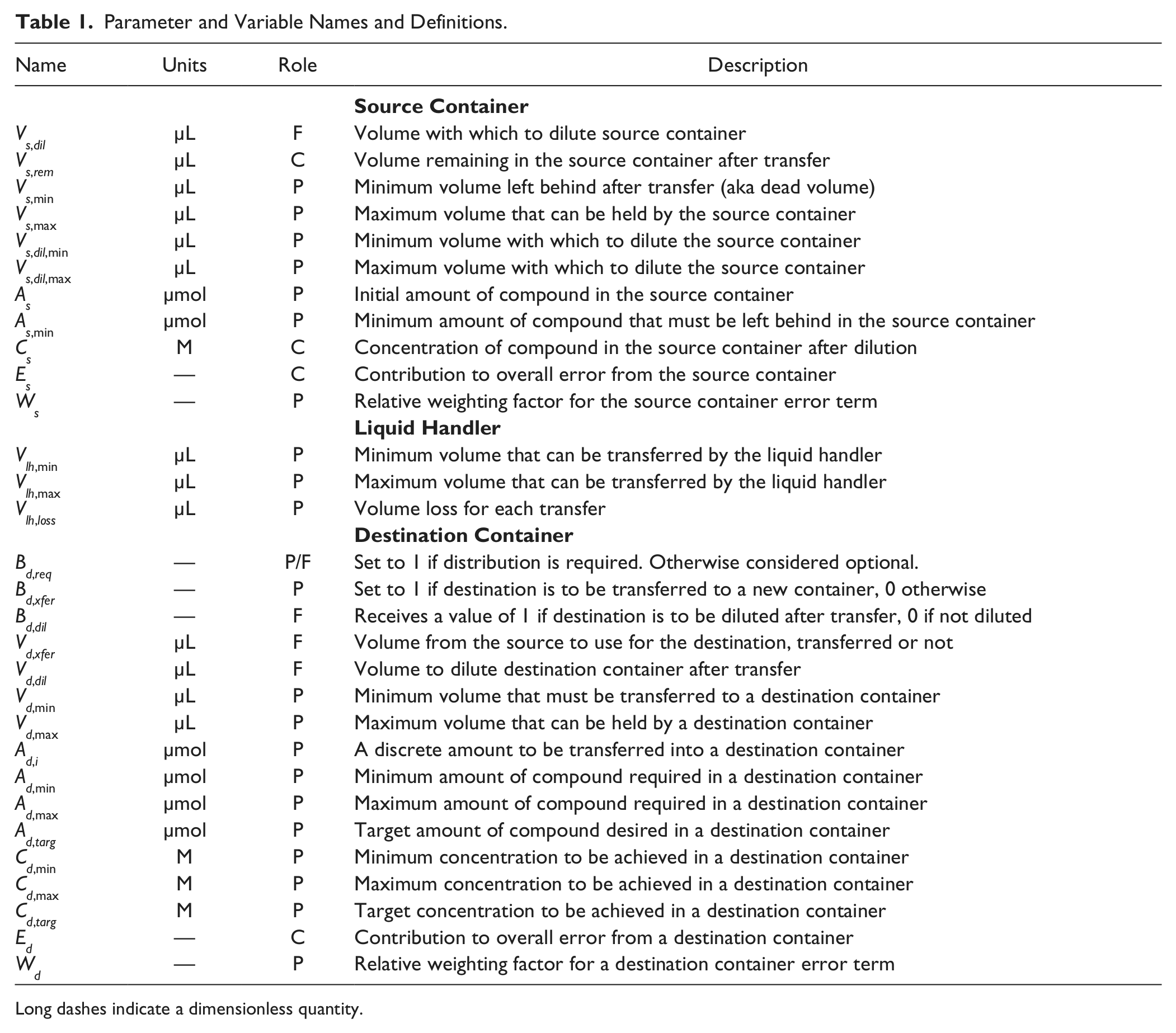
Long dashes indicate a dimensionless quantity.

Source Container

All distributions start with the source container holding the sum total of all compound available. Table 2 lists all source container parameters with default values and whether each is required (Y) or not (N).

Table 2.

Source Container Parameters.

Name	Default	Required	Additional Notes and Requirements
V_s,min	0.0	N	≥0.0
V_s,max	—	Y	≥V_s,min
V_s,dil,min	0.0	N	≥V_s,min
V_s,dil,max	V_s,max	N	≤V_s,max
A_s	—	Y	≥0.0
A_s,min	0.0	N	≥0.0
W_s	1.0	Y	Used to indicate relative importance of driving volume to 0.0

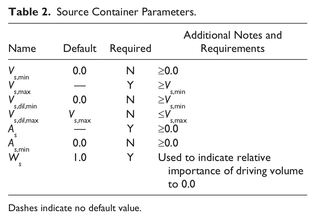
Dashes indicate no default value.

The source container specification begins with the definition of the source concentration, which is the ratio of the original amount of compound in the container and the dilution volume, equation (1).

C_{s} = \frac{A_{s}}{V_{s, d i l}}

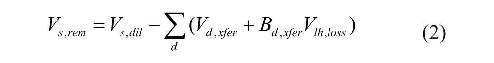
The volume that remains in the source container is the initial dilution volume minus all transfers performed to fulfill distributions, equation (2). Recall that it is not necessary for all distributions to be transferred; one may remain in the source container. This leave-behind distribution is specified by setting its B_d,xfer Boolean parameter to 0. Also important to take into consideration is the volume loss that may be incurred during each transfer, V_lh,loss. In equation (2), this volume loss is multiplied by the Boolean value indicating if the distribution is to be transferred. This ensures that the transfer loss is subtracted only when the distribution is transferred.

V_{s, r e m} = V_{s, d i l} - \sum_{d} (V_{d, x f e r} + B_{d, x f e r} V_{l h, l o s s})

The volume remaining in the source container must be greater than or equal to the maximum of two volumes: the minimum volume that must be left in the container and the minimum volume with which to dilute the source container, equation (3).

V_{s, r e m} \geq \max (V_{s, \min}, V_{s, d i l, \min})

The minimum amount of compound that must remain in the source container must be less than the actual amount, which is computed as the source container concentration times the remaining volume, equation (4).

A_{s, \min} \leq C_{s} V_{s, r e m}

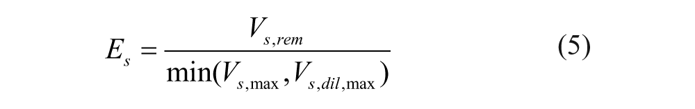
The error term for the source container is the volume remaining after all transfers are completed, divided by the maximum volume that the container can hold, which is the minimum of the maximum container volume and the maximum dilution volume, equation (5). This is one among several error terms whose total sum is minimized to obtain a problem solution, equation (31).

E_{s} = \frac{V_{s, r e m}}{\min (V_{s, \max}, V_{s, d i l, \max})}

Variable Amount Distribution

Being the simplest of distribution types, the variable amount distribution specifies constraints only on the volume and amount of compound required to fulfill the distribution. Table 3 describes all parameters for a variable amount distribution.

Table 3.

Variable Amount Distribution Parameters.

Name	Default	Required	Additional Notes and Requirements
V_d,min	0.0	N	≥0.0
V_d,max	—	Y	≥V_d,min
A_d,min	—	Y	≥0.0
A_d,max	—	Y	≥A_d,min
A_d,targ	—	N	Ignored if not specified
B_d,req	0	N	By default, distribution is not required (i.e., optional)
B_d,xfer	1	N	By default, distribution will be transferred into a new container
W_d	1.0	N	Used to indicate the relative importance of achieving A_d,targ, if specified

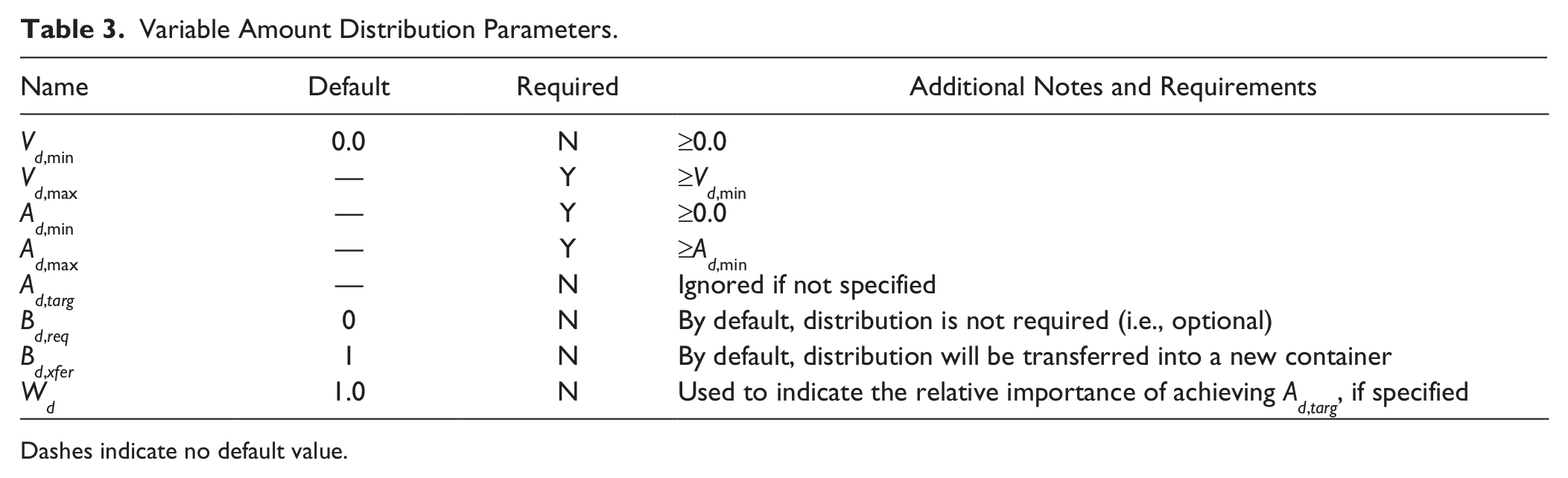
Dashes indicate no default value.

If the distribution is to be transferred to a new container, then equations (6) and (7) are added to the problem formulation. If the distribution is to be left behind in the source container (B_d,xfer = 0), then only equation (8) is added to the problem formulation.

The transfer volume from the source container to the destination for the distribution must be less than the minimum of the maximum liquid handler transfer volume and the maximum destination container volume, equation (6).

V_{d, x f e r} \leq B_{d, r e q} \min (V_{l h, \max}, V_{d, \max})

The transfer volume also must be greater than the maximum of the minimum liquid hander transfer volume and the minimum destination container volume, equation (7).

V_{d, x f e r} \geq B_{d, r e q} \max (V_{l h, \min}, V_{d, \min})

When the distribution is to be left behind in the source container (B_d,xfer = 0), the volume remaining in the source container must equal the distribution volume, equation (8).

V_{d, x f e r} = V_{s, r e m}

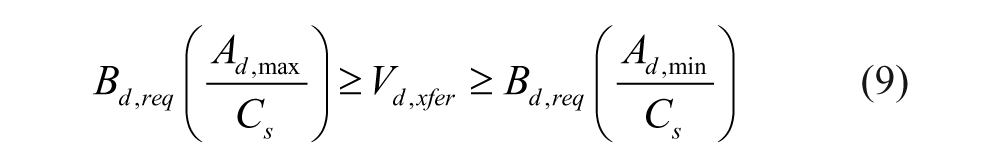
If the distribution is to be transferred to a new container (B_d,xfer = 1) and destination container amount limits are specified, then the following two constraints are applied, equation (9).

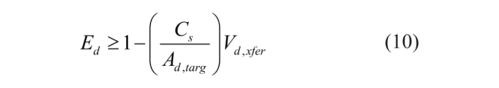
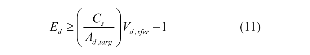
B_{d, r e q} (\frac{A_{d, \max}}{C_{s}}) \geq V_{d, x f e r} \geq B_{d, r e q} (\frac{A_{d, \min}}{C_{s}})

If a target amount is specified, then the error term should drive the amount of the distribution toward the optimum. This is achieved by using a linearization technique that sets up two constraints, equations (10) and (11), into a V-shaped region with a minimum value (bottom of the “V”) at the target transfer amount. If a target amount is not specified, these constraints are excluded.

E_{d} \geq 1 - (\frac{C_{s}}{A_{d, t a r g}}) V_{d, x f e r}

E_{d} \geq (\frac{C_{s}}{A_{d, t a r g}}) V_{d, x f e r} - 1

Concentration Range Distribution

This distribution type is characterized by upper and lower limits on the concentration of compound in the destination container. In addition, standard volume constraints are applied, which reflect the limits of the destination container and liquid handler. Parameters are listed in Table 4 .

Table 4.

Concentration Range Distribution Parameters.

Name	Default	Required	Additional Notes and Requirements
V_d,min	0.0	N	≥0.0
V_d,max	—	Y	≥V_d,min
C_d,min	—	Y	≥0.0
C_d,max	—	Y	≥C_d,min
C_d,targ	—	N	Ignored if not specified
B_d,req	0	N	By default, distribution is not required (i.e., optional)
B_d,xfer	1	N	By default, distribution will be transferred into a new container
W_d	1.0	N	Used to indicate the relative importance

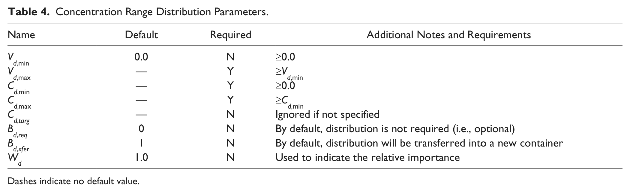
Dashes indicate no default value.

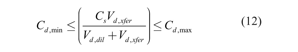
The concentration of the compound in the destination container must fall within the specified limits, equation (12). Note that the dilution volume V_d,dil represents the volume of solvent to be added to the destination container after the compound solution is transferred. With this feature, a more concentrated solution can be made in the source container and subsequently diluted so that it falls within the required range.

C_{d, \min} \leq (\frac{C_{s} V_{d, x f e r}}{V_{d, d i l} + V_{d, x f e r}}) \leq C_{d, \max}

If the distribution is to be transferred into a destination container (B_d,xfer = 1), equations (13) through (17) are included in the problem formulation. If the distribution is to remain in the source container (B_d,xfer = 0), equations (18) through (21) are included instead.

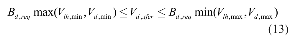
The transfer volume must fall within the maximum of the minimum liquid hander volume and minimum container volume, as well as the minimum of the maximum liquid hander volume and maximum container volume, equation (13). Also note that the constraints are multiplied by the Boolean B_d,req, which may be treated as a parameter or a free variable. If B_d,req is set to 1, the distribution is required and the concentration constraints are enforced. If the variable is left as a free variable, then the distribution is optional and B_d,req may change between 0 and 1 in an attempt to find the optimum solution. A value of 0 causes the distribution to be excluded by requiring that the final concentration have a value of 0.

B_{d, r e q} \max (V_{l h, \min}, V_{d, \min}) \leq V_{d, x f e r} \leq B_{d, r e q} \min (V_{l h, \max}, V_{d, \max})

The sum of the transfer and dilution volumes must be less than the total container destination volume, equation (14).

V_{d, x f e r} + V_{d, d i l} \leq B_{d, r e q} V_{d, \max}

The dilution volume must be greater than the minimum liquid handler transfer volume and less than the maximum liquid handler transfer volume, equation (15). Note the use of B_d,req, which can be either a parameter or a free variable. If B_d,req is set to 1, the volume range is enforced. If it is not set, the value of B_d,req is free to change between 0 and 1. When it has a value of 0, the dilution volume must also be 0.

B_{d, r e q} V_{l h, \min} \leq V_{d, d i l} \leq B_{d, r e q} V_{l h, \max}

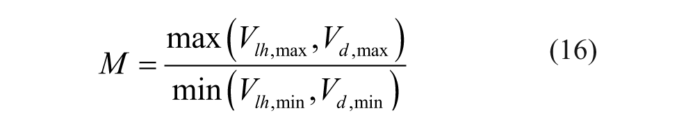
Finally, if the transfer volume V_d,xfer equals 0, then the dilution volume V_d,dil must be forced to a value of 0, because there is no reason to dilute a container with no compound. To accomplish this, we use a standard technique called the “Big M” method of linear programming, described in the following. We start by computing a parameter called M that is guaranteed to be much larger than the ratio of V_d,dil/V_d,xfer. In this case, the smallest volume that is transferred into the destination container can be no less than the minimum of the smallest liquid handler transfer volume and the smallest volume that the destination can hold. Likewise, the largest volume that is transferred into the destination can be no greater than the maximum of the largest liquid handler transfer volume and the largest volume that can be held by the destination container. The ratio of these two values is called M and is defined by equation (16). This ratio will always be larger than or equal to the ratio V_d,dil/V_d,xfer, which can be expressed as equation (17). Note that when the transfer volume is greater than 0, equation (17) is easily satisfied. When the transfer volume equals 0, equation (17) forces the dilution volume to 0.

M = \frac{\max (V_{l h, \max}, V_{d, \max})}{\min (V_{l h, \min}, V_{d, \min})}

V_{d, d i l} \leq M V_{d, x f e r}

When a concentration range distribution is to remain in the source container (B_d,xfer = 0), the volume remaining after all transfers must be one and the same, equation (18).

V_{d, x f e r} = V_{s, r e m}

The sum of the volume left behind in the source container and the dilution volume computed must not exceed the maximum volume that can be held by the source container, equation (19).

V_{s, \max} \geq V_{d, x f e r} + V_{d, d i l}

The dilution volume must be greater than the minimum liquid handler transfer volume; otherwise, it must be zero, equation (20).

V_{d, d i l} \geq B_{d, d i l} V_{l h, \min}

Likewise, the dilution volume must be less than the maximum container volume; otherwise, it must be zero, equation (21).

V_{d, d i l} \leq B_{d, d i l} V_{l h, \max}

The goal of this distribution type is to drive the overall volume to be as low as reasonable. We want to avoid diluting the container, if possible. To accomplish this, we use the linear V-shaped constraint technique that has an error 0.0 when the container volume reaches its minimum value, expressed as equations (22) and (23).

E_{d} \geq 1 - (\frac{V_{d, x f e r} + V_{d, d i l}}{V_{d, \min}})

E_{d} \geq (\frac{V_{d, x f e r} + V_{d, d i l}}{V_{d, \min}}) - 1

Discrete Amount Distribution

In certain scenarios, exact amounts are required for a given compound distribution. For example, it is not uncommon to plan for a set of compounds to be tested in several assays, each of which is contingent upon the required amount of compound being available. A primary assay is performed upfront, which demands a prespecified amount of compound. Depending on the results of this assay, a second assay may be performed, only if there is sufficient compound left over. The second assay also demands a certain amount of compound; therefore, the distribution container must contain either the amount of compound required for the first assay or a larger amount that is the sum total required for both assays. Anything above the amount needed for the first assay but below the amount needed for both would be wasted. This scenario can be handled with the discrete amount distribution. Table 5 lists all parameters required for performing a discrete amount distribution.

Table 5.

Discrete Amount Distribution Parameters.

Name	Default	Required	Additional Notes and Requirements
V_d,min	0.0	N	≥0.0
V_d,max	—	Y	≥V_d,min
A_d,i	—	Y	Identifies a sequence of increasing amounts that may be distributed, i = 1 to max
A_d,targ	—	N	Desired amount for distribution
B_d,req	0	N	By default, distribution is not required (i.e., optional)
B_d,xfer	1	N	By default, distribution will be transferred into a new container
W_d	1.0	N	Used to indicate the relative importance of achieving A_d,targ

Dashes indicate no default value.

A sequence of increasing discrete compound amounts parameterizes a discrete amount distribution. The distribution begins by attempting to fulfill the first amount in the sequence. If this is achieved, then a larger second distribution is attempted. This continues for all increasing discrete target amounts, which are specified as the A_d,i parameter set—the N-element sequence of values named A_d,1, A_d,2, . . ., A_d,N.

The final mathematical problem statement is constructed by starting with the initial amount (A_d,1) and then adding incremental amounts that leave open the possibility of achieving larger values in the sequence. The initial amount and all subsequent incremental amounts are multiplied by Boolean parameters from the set B_d,i, which are used to test if the next discrete amount in the sequence can be fulfilled. The resulting mathematical statement looks like the following:

Amount transferred = B_{d, r e q} A_{d, 1} + B_{d, 2} (A_{d, 2} - A_{d, 1}) + B_{d, 3} (A_{d, 3} - A_{d, 2}) + \dots + B_{d, N} (A_{d, N} - A_{d N - 12})

Note that the first amount in the series is multiplied by B_d,req, the Boolean parameter that indicates whether the minimum value in the distribution is required. When B_d,req = 1, the minimum amount of A_d,1 must be fulfilled. When B_d,req is not set, it is a free variable whose value is free to change between 0 and 1.

This constraint alone is not sufficient to ensure the desired outcome. If any Boolean variable in the B_d,i sequence has a value of 1, then all previous values in the sequence must also be 1. For example, it is not acceptable for B_d,2 to be assigned a value of 1 before B_d,req. To enforce this condition, the additional series of constraints is added to the mathematical problem formulation, equation (24) .

B_{d, r e q} > B_{d, 2}, B_{d, 2} > B_{d, 3}, \dots, B_{d, N - 1} > B_{d, N}

In practice, rather than using distribution amounts, volumes are constrained. The actual constraints added to the problem formulation divide amounts by the source container concentration for volume terms. The resulting constraint is constructed as in equation (25).

V_{d, x f e r} = B_{d, r e q} \frac{A_{d, 1}}{C_{s}} + \sum_{i = 2}^{n - 1} B_{d, i} \frac{A_{d, i} - A_{d, i - 1}}{C_{s}}

If the distribution is to be left behind in the source container (B_d,xfer = 0), then the volume remaining in the source container is equal the distribution volume, equation (26).

V_{d, x f e r} = V_{s, r e m}

If the distribution is to be transferred into a new container (B_d,xfer = 1), then the standard destination container constraints are added to the mathematical formulation, equations (27) and (28).

V_{d, x f e r} \leq B_{d, r e q} \min (V_{l h, \max}, V_{d, \max})

The transfer volume also must be greater than the maximum of the minimum liquid hander transfer volume and the minimum destination container volume.

V_{d, x f e r} \geq B_{d, r e q} \max (V_{l h, \min}, V_{d, \min})

If a target amount is specified, then equations (29) and (30) will drive the amount of the distribution toward this optimal target value.

E_{d} \geq 1 - (\frac{C_{s}}{A_{d, t a r g}}) V_{d, x f e r}

E_{d} \geq (\frac{C_{s}}{A_{d, t a r g}}) V_{d, x f e r} - 1

Solution

Setting up a problem that solves for a set of compound distributions starts by selecting the number and type of distributions to be fulfilled. Frequently, business rules dictate a standard set of distributions that are to be created, if sufficient compound is available. After the distributions are identified, all parameter values are set. Parameter values associated with the source container and liquid handler are set first, such that all parameters in equations (1) through (5) are assigned, leaving V_s,dil, V_s,rem, and C_s to be computed. All resulting substituted constraints are collected and added to the problem specification.

The next step is to set distribution parameter values. For all variable amount distributions, the primary variable to be determined is V_d,xfer. The parameter B_d,req is either set to 1 if the distribution is required or left unassigned as a second variable if it is optional. Everything else is a parameter that must have a value specified upfront. Equations (6), (7), (10), and (11) are added to the problem specification. Equation (9) is added if the distribution is to be transferred to a new destination container. If the distribution is the single distribution that is to be left behind in the source container, equation (8) is used instead of equation (9).

For all concentration range distributions, V_d,xfer and V_d,dil are both left as variables. B_d,req is set to 1 if the distribution is required or left unassigned as a second variable if it is optional. Equations (13), (22), and (23) are added to the problem specification for each concentration range distribution. Equations (13) through (17) are added to each if it is to be transferred into a destination container, and equations (18) through (21) are added if a distribution is to remain in the source container.

For all discrete amount distributions, V_d,xfer is left as a variable. B_d,req is set to 1 if the distribution is required or left unassigned as a second variable if it is optional. For each distribution of this type, two sets of inequalities are added to the problem specification as described by equations (24) and (25). Equations (29) and (30) are added for each distribution as well. Equations (27) and (28) also are added if a distribution is to be transferred into a destination container; otherwise, equation (26) is added if a distribution is to remain in the source container.

The final step required to complete a problem specification is to assemble the equation that defines total error, E_T. This is the term that will be minimized in an attempt to find the optimal solution. E_T is the sum of all error terms, one for the source container and one for each destination container that has a target amount. Only variable amount distribution or discrete amount distribution types have optional target amount parameters. When no target amount is specified there is no error term. The total error is defined as the weighted sum of the source error and all distribution errors, given as equation (31).

E_{T} = W_{s} E_{s} + \sum_{d} W_{d} E_{d}

The final assembled problem is made up of the collection of all substituted constraints from the source and all destination containers along with the equation for total error. The number of variables that must be managed can be significant. Automating the assembly of the mathematical problem specification is a prerequisite if this technique is to be applied on a regular basis. We solved this problem by writing a computer program that reads a configuration file that specifies all distributions to be made and all parameter values. The program automatically assembles the mathematical problem statement and solves the problem returning either the optimal solution or a message indicating that there exists no feasible solution that simultaneously satisfies all constraints.

Many of the generated constraints are nonlinear, which substantially increases the complexity of the computation. Fortunately, the class of problems generated by this technique can be made linear by holding one variable constant—namely, the source container dilution volume V_s,dil. With a constant value for V_s,dil, a linear programming technique can be used to solve the linearized problem quickly and efficiently. Of course, in the more general problem, V_s,dil is a variable whose value must also be optimized. To address this issue, we employed a hybrid numerical solver composed of a nonlinear optimizer that works to minimize total error, equation (31), by modifying only the value for V_s,dil. The objective function for the optimizer is the linear program that computes a solution for the linearized problem obtained when a trial value for V_s,dil is chosen. This hybrid numerical technique has proved to be fast and reliable.

Example

To illustrate our technique, consider a source container initially holding 10 µmol of dry compound from which we would like to create six total distributions. Five distributions are to be transferred into new containers and one is to remain in the source container. All parameters for the source container, liquid handler, and all six distributions are summarized in Table 6 . Note that the six distributions are given the unique names Discrete Amt-1, Discrete Amt-2, Discrete Amt-3, Variable Amt-4, Variable Amt-5, and Conc Range-6. These are listed in the header row of the table. The leftmost column contains each parameter name. We have combined several related variables in the same table row to save space. For example, the parameter named V_(s/lh/d),min indicates that the table row shows V_s,min for the source container column, V_lh,min for the liquid handler column, and V_d,min for all distribution columns. Each of the remaining columns in the table is used for one of the containers involved in the distribution: source, liquid handler, and the six distributions. Note that table cells are assigned values only when it makes sense for the distribution type.

Table 6.

Example Problem Parameter Values.

Parameter	Source Container	Liquid Handler	Discrete Amt-1	Discrete Amt-2	Discrete Amt-3	Variable Amt-4	Variable Amt-5	Conc Range-6
W_(s/d)	8		7	6	5	1	1	9
B_d,req			1	—	—	—	1	1
B_d,xfer			1	1	1	1	0	1
V_(s/lh/d),min	1000.0	25.0	100.0	100.0	100.0	100.0	100.0	25.0
V_(s/lh/d),max	12,000.0	2400.0	2900.0	2900.0	2900.0	2900.0	10,000.0	2900.0
V_lh,loss		1.0
V_s,dil,min	1000.0
V_s,dil,max	12,000.0
A_s	10.0
A_(s/d),min	0.0					1.0	1.0
A_d,max						30.0	2.0
A_d,targ						30.0	2.0
A_d,1			0.42	1.24	1.0
A_d,2			2.74	3.08	4.0
C_d,min								0.0005
C_d,max								0.001
C_d,targ								0.001

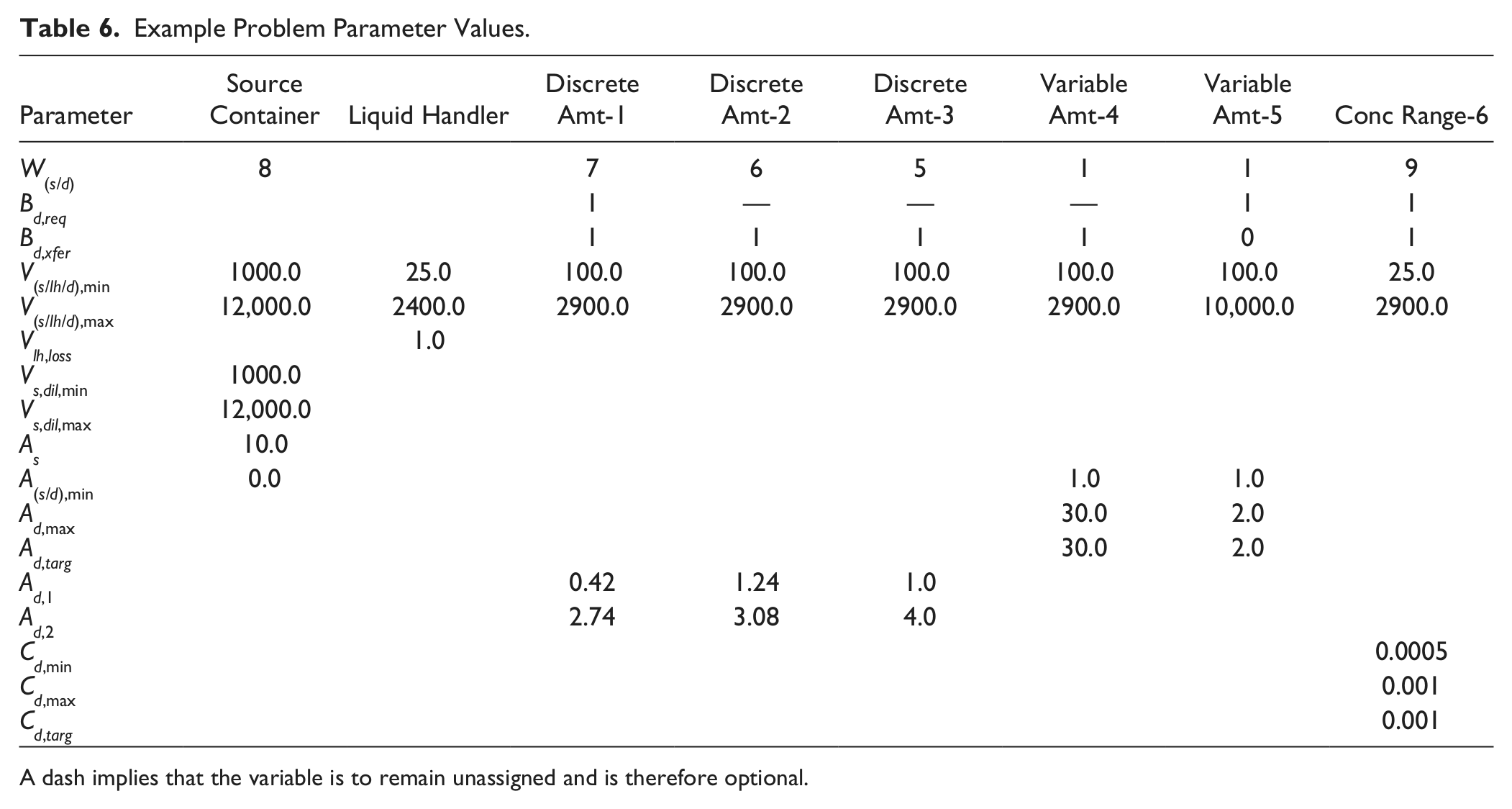
A dash implies that the variable is to remain unassigned and is therefore optional.

This example problem has a few special attributes worth noting. The first row labeled W_(s/d) lists error term weights for each container. Weight magnitudes roughly indicate the relative importance of minimizing the error term for each container. It is important to note that it may be necessary to adjust weight values to achieve results that match business rules. In our example, we gave the Conc Range-6 distribution a relatively large weight of 9, indicating our preference that this container reach its target concentration before, for example, the variable amount distributions Variable Amt-4 and Variable Amt-5, which have a lower weight value of 1.

Recall that a B_d,req Boolean parameter is set to 1 if the distribution must be performed. Leaving the variable unassigned implies that the distribution is optional. Only the Discrete Amt-1, Variable Amt-5, and Conc Range-6 distributions are required for this example problem. All other distributions are optional and will be fulfilled only after the required distributions are fulfilled and if there is sufficient compound remaining.

All B_d,xfer parameters are set to 1 except that for the Variable Amt-5 distribution, which is set to 0. This indicates that the Variable Amt-5 distribution is not to be transferred into a new container. It will be left behind in the source container.

Maximum and minimum volume parameters are specified for all containers and distributions. Also, each discrete amount distribution is set up with a sequence of two discrete amounts that are to be fulfilled, named A_d,1 and A_d,2. Because Discrete Amt-1 is a required distribution, its first discrete amount of 0.42 µmol must be fulfilled. The remaining two discrete amount distributions may end with a value of 0 µmol as well as their two listed discrete amounts because they are marked as being optional.

Assembling the problem statement starts by collecting the constraints for each container and distribution, substituting parameters, and assembling a total weighted error equation. To solve the problem, a trial source container dilution volume (V_s,dil) is selected and substituted, making all constraints linear. A linear programming solver is used to solve the substituted set of constraints in such a way as to minimize total error at the given source container dilution volume. This process is repeated with new trial dilution volumes until the total error is minimized in a global sense, over all possible source container dilution volumes. Figure 1 is a plot of total error (31) as a function of dilution volume. For this example problem, the minimum total error occurs at a dilution volume of exactly 5000 µL. It is interesting to note that a second local minimum occurs at 10,000 µL. There is some interesting behavior of total error between dilution volumes of about 7500 µL and 10,000 µL. Source container dilution volumes outside the range [1643 µL, 10,000 µL] are infeasible, meaning no solution exists that will satisfy all required constraints.

Figure 1.

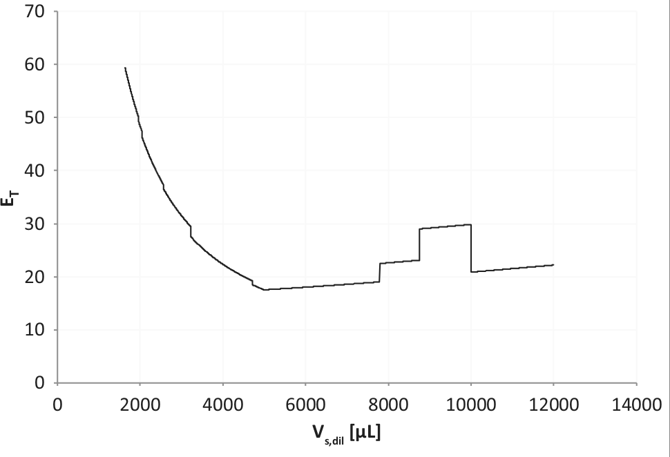
Total error as a function of source container dilution volume.

To better comprehend how the curve in Figure 1 arises, consider the curves in Figure 2 . The seven error terms from the example are plotted against source container dilution volume in such a way as to reveal their individual contributions to total error (E_T). Each consecutive error term is added to the sum of all previously plotted terms. This incremental sum is the value that is ultimately plotted for a given error. The result is a kind of stacked chart, where the topmost curve represents the sum of all error terms. The order in which the terms are summed and plotted is given as the legend of Figure 2 , starting with the error due to the source container, “E (Source).” By the time we reach the last error term, “E (Conc Range-6),” the incremental error sum is equivalent to the total error.

Figure 2.

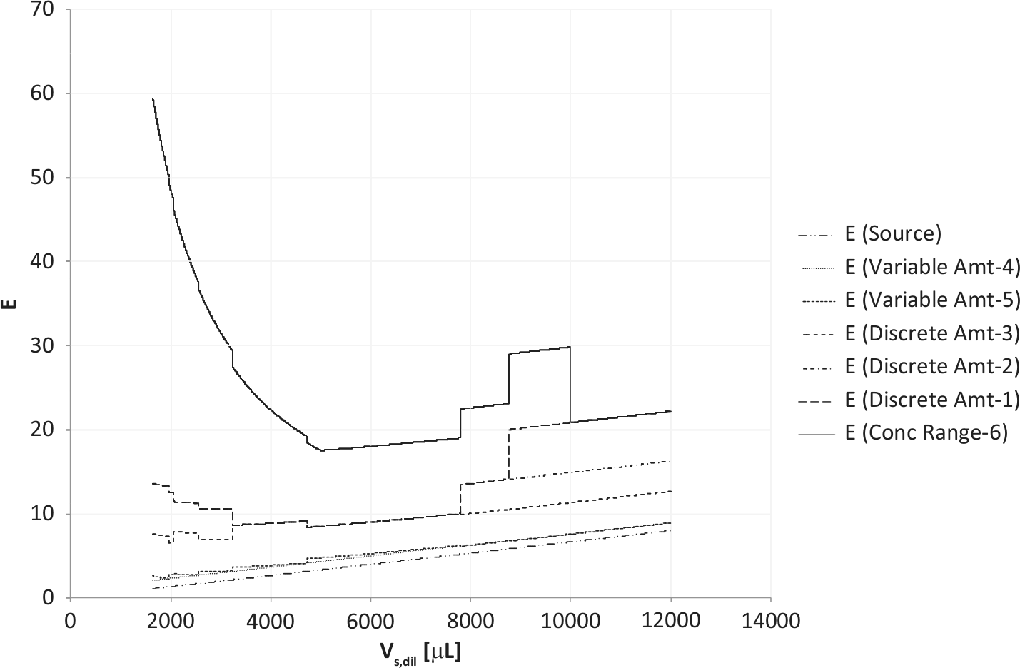
All error terms, incrementally summed, as a function of source container dilution volume.

The first curve at the bottom of the chart with a short-dash two-dot pattern (-..) and labeled “E (Source)” is the error due to the source container (E_S). The second curve on the chart labeled “E (Variable Amt-4)” with a dot pattern (. . .) is the error term for the Variable Amt-4 distribution added to the error due to the source container, just below it. Following this pattern, the error term for Variable Amt-5 is added to the previous sum and plotted as “E (Variable Amt-5),” a curve with a compact short dash pattern (---). This continues with “E (Discrete Amt-3)” having a spaced short dash pattern (---), “E (Discrete Amt-2)” having a dash-dot pattern (- .), “E (Discrete Amt-1)” having a long dash pattern (— — —), and “E (Conc Range 6)” plotted as the topmost solid line pattern.

The “E (Source)” curve increases linearly to the right as the source container dilution volume increases. The “E (Variable Amt-4)” and “E (Variable Amt-5)” curves add only incrementally to the overall error, which is consistent with the fact that their weights are relatively small, each having a value of 1. The “E (Discrete Amt-3),” “E (Discrete Amt-2),” and “E (Discrete Amt-1)” curves are interesting, showing discrete changes in value at various points as dilution volume increases. This explains the comparable behavior of the total error curve in Figure 1 . By careful inspection, it is possible to identify which sample is responsible for the total error curve features. The final “E (Source)” curve starts with large values at the lowest dilution volume and decreases until it reaches a value of 0 at a dilution volume of 10,000 µL. This term is almost entirely responsible for the large total error at low dilution volumes and the gradual decrease as dilution value increases. We have found that a chart such as the one in Figure 2 is valuable for tuning the weight values for a given problem.

The three discrete amount distributions (Discrete Amt-1, Discrete Amt-2, and Discrete Amt-3) exhibit complex behavior as source dilution volume changes. Figure 3 plots transfer volumes required to fulfill each discrete amount distribution as a function of source container dilution volume. This behavior is better appreciated by referring to Figure 4 , which plots the amount of compound distributed instead of transfer volume as a function of source dilution volume. The amount of compound transferred is calculated by multiplying transfer volume by the source container concentration at the current dilution.

Figure 3.

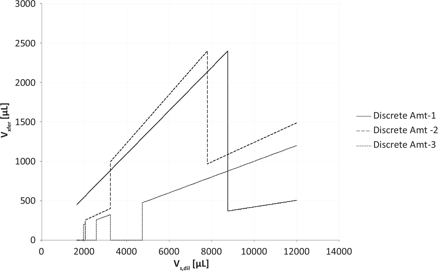
Transfer volume for the three discrete amount distributions as a function of source container dilution volume.

Figure 4.

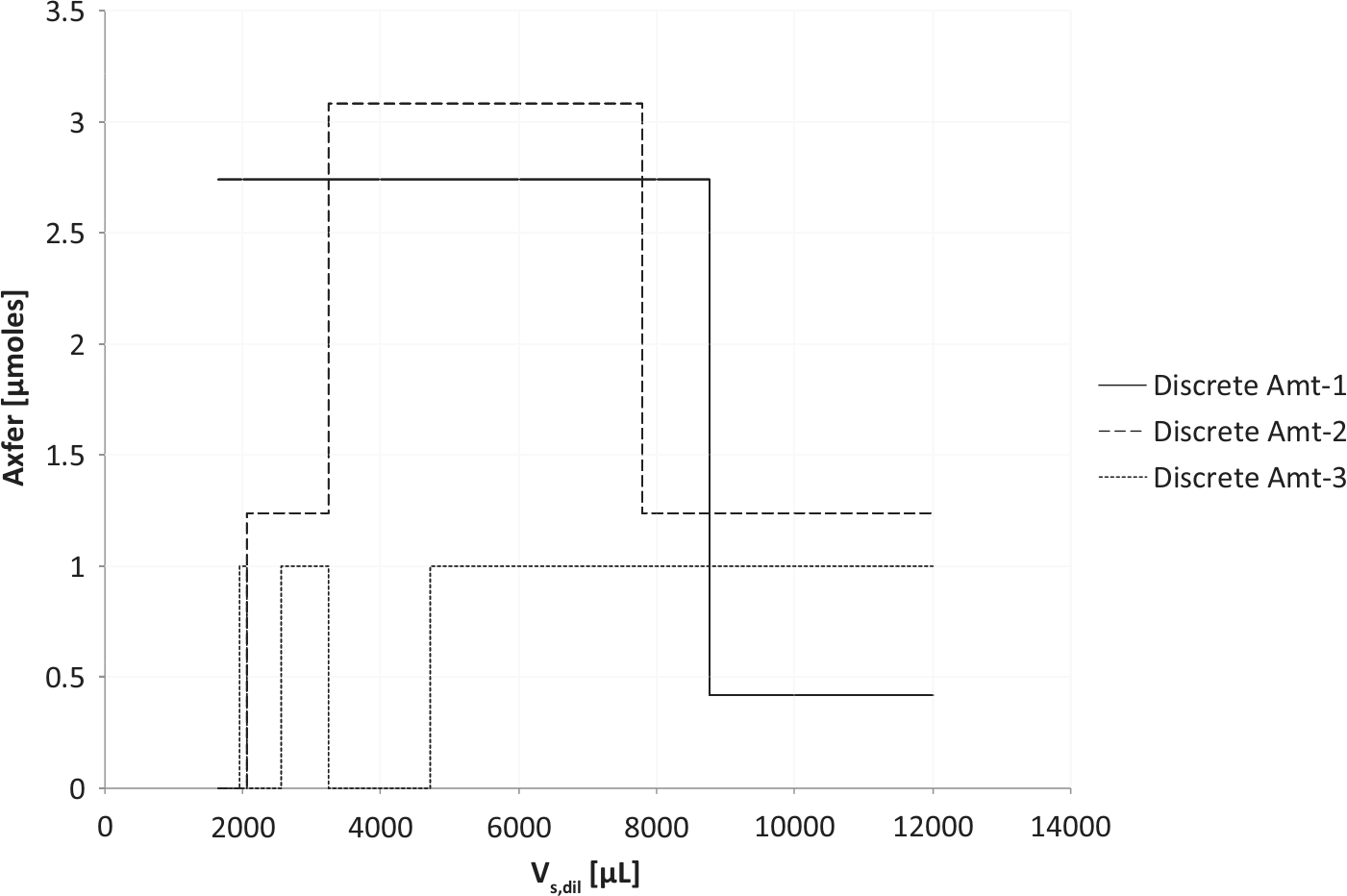
Transfer amount for the three discrete amount distributions as a function of source container dilution volume.

The smallest feasible source container dilution volume is 1643 µL. At this volume, only A_d,1 for the Discrete Amt-1 distribution can be fulfilled at the higher amount of 2.74 µmol. Between a source dilution volume of 1957 µL and 2049 µL, Discrete Amt-3 can be fulfilled as well. At 2050 µL, Discrete Amt-2 is fulfilled with an amount of 1.24 µmol in favor of Discrete Amt-3. Only one of the two distributions is possible at this volume. Because the weight parameter for Discrete Amt-2 is greater than that for Discrete Amt-3, Discrete Amt-2 takes priority. At 2563 µL, both Discrete Amt-2 and Discrete Amt-3 can be fulfilled, with Discrete Amt-3 once again at the lower amount of 1 µmol. At 3236 µL, the best solution dictates that Discrete Amt-3 once again be removed in favor of the higher distribution value of 3.08 µmol for Discrete Amt-2. At 4725 µL, Discrete Amt-3 is reintroduced in the best solution for a third time at 1 µmol. This continues until 7793 µL, at which point the amount of Discrete Amt-2 drops from 3.08 to 1.24 µmol. The last change occurs at 8760 µL, where the amount for the Discrete Amt-1 distribution drops from its higher value of 2.74 to 0.42 µmol, where it remains until no distribution is feasible at the maximum source dilution volume of 10,000 µL.

Figure 5 illustrates compound amounts computed for both the Variable Amt-4 and Variable Amt-5 distributions. Both variable amount distributions have equal weight values of 1. Recall that the Variable Amt-5 distribution has a minimum amount constraint of 1 µmol and a maximum of 2 µmol. These bounds are reflected in the computed results. As source dilution volume increases, amount values computed for Variable Amt-5 fluctuate in a jigsaw pattern between the lower 1-µmol and upper 2-µmol bounds. At a source container dilution volume of 7793 µL, the Variable Amt-5 distribution jumps to its maximum value of 2 µmol, where it remains until the 12,000-µL maximum dilution is reached. Also at 7793 µL, the optional Variable Amt-4 distribution is able to be fulfilled and switches from 0 µmol to an initial value of 1.697 µmol. The Variable Amt-4 distribution amount also fluctuates as dilution volume increases, reaching a value as high as 2.74 µmol before settling at 2.0 µmol at the maximum dilution of 12,000 µL.

Figure 5.

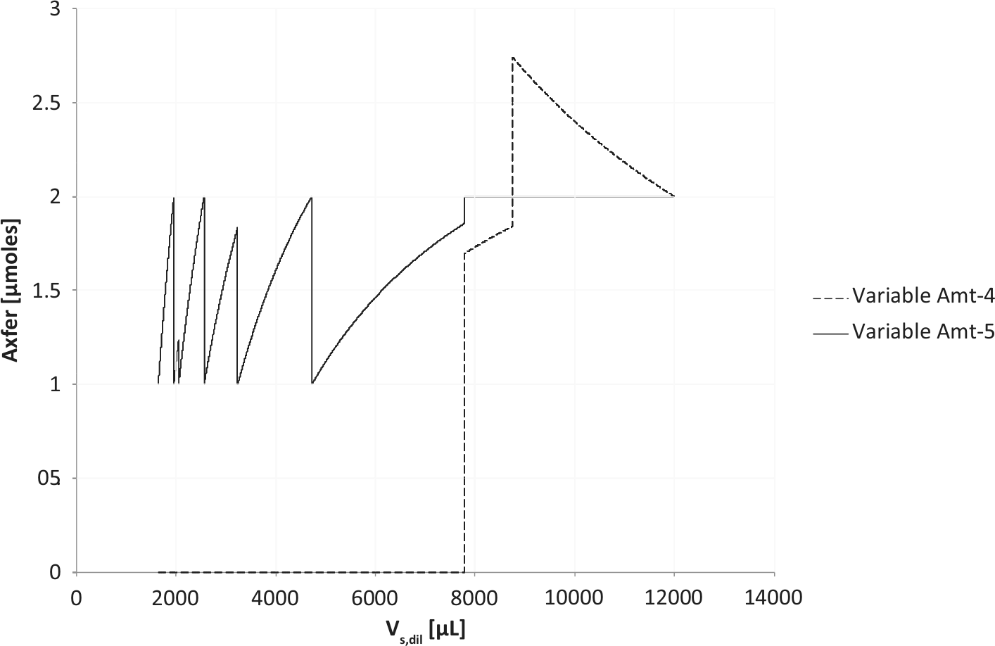
Transfer amount for the two variable amount distributions as a function of source container dilution volume.

Behavior of the Conc Range-6 distribution is illustrated in Figure 6 . The transfer volume (V_d,xfer) and dilution volume (V_d,dil) are plotted on the left vertical axis, and final concentration (C_d) is plotted on the right vertical axis. The Conc Range-6 distribution has a weight value of 9, the largest weight in the problem formulation. The target concentration (C_d,targ) and maximum concentration (C_d,max) of the distribution has a value of 1.0 µM, with a minimum concentration (C_d,min) of 0.5 µM. The target concentration is achievable up to a source dilution volume of 5000 µL. Between 5000 µL and 10,000 µL, the concentration must be reduced. At 10,000 µL, it returns to its target value of 1.0 µM, after which it is reduced again until it reaches 0.833 µM at the maximum source dilution of 12,000 µL.

Figure 6.

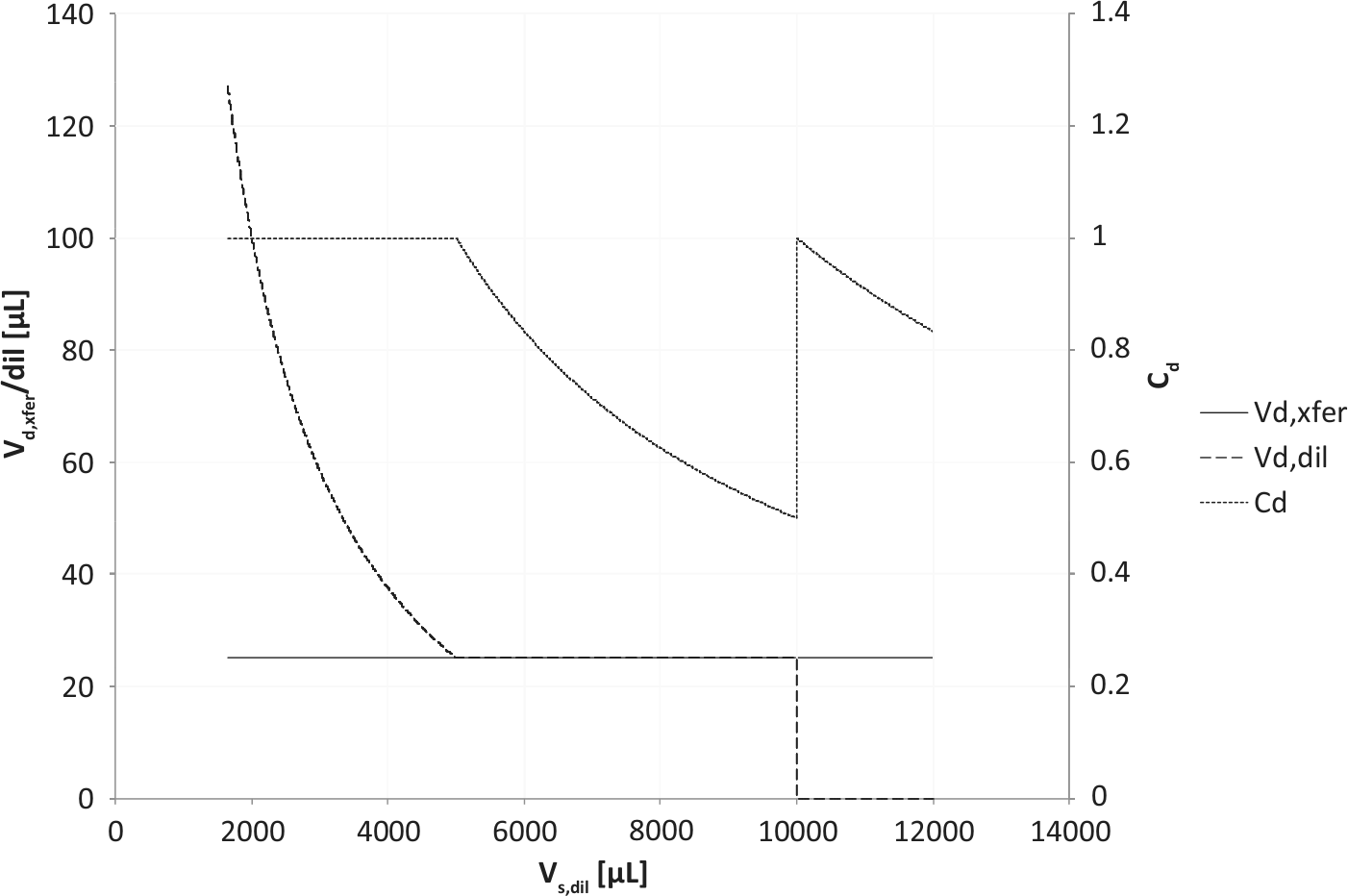
Transfer volume and concentration for the Conc Range-6 distribution as a function of source container dilution volume.

The final set of optimal transfer and dilution volumes for all distributions are those computed when the total error (E_T) reaches a minimum at a source container dilution volume of 5000 µL. The distributions fulfilled and volumes computed can be modified by changing distribution weight values to better reflect business rules.

In conclusion, the method presented for formulating and solving complex compound distribution problems is a powerful technique that builds on and extends earlier work.² Successfully following the procedure that has been outlined requires the careful management of numerous details. For that reason, we have implemented a software program that carries out the problem formulation and numerical solution. The program reads a configuration file containing a complete problem specification, automatically assembles the mathematical problem based on parameter values provided, and solves the problem numerically, returning the optimal feasible solution or no solution when one does not exist. Standard numerical libraries are used to solve the formulated problem.

Of particular interest is the rich and unpredictable solutions obtained for all distributions as the source container dilution volume changes. Interesting fluctuations in transfer and dilution volumes required to satisfy all distributions are demonstrated in the example problem that has been explored in detail. Due to the unpredictability of the results, it is clear that this computational approach generates interesting opportunities to maximize the utilization of scarce compounds that would be unattainable using only a trial-and-error approach.

Footnotes

Declaration of Conflicting Interests

The authors declared no potential conflicts of interest with respect to the research, authorship, and/or publication of this article.

Funding

The authors received no financial support for the research, authorship, and/or publication of this article.

References

Weller

H. N.

Nirschl

D. S.

Paulson

J. L.

Hoffman

S. L.

Bullock

W. H.

Addressing the Medicinal Chemistry Bottleneck: A Lean Approach to Centralized Purification. ACS Comb. Sci. 2012, 14, 520–526.

Russo

M. F.

Hoffman

S. L.

Determining Feasibility and Parameter Values for Compound Orders Based on Transfer Amounts, Liquid Handler Capabilities, and Container Volume Capacities. J. Assoc. Lab. Autom. 2001, 6, 77–85.

A Computational Method for Planning Complex Compound Distributions under Container,Liquid Handler,and Assay Constraints

Abstract

Keywords

Introduction

Model Problem

Constraints

Source Container

Variable Amount Distribution

Concentration Range Distribution

Discrete Amount Distribution

Solution

Example

Footnotes

Declaration of Conflicting Interests

Funding

References