Effect of Household Structure Changes on Consumption Inequality: An Empirical Study from Household Data in China

Abstract

Based on the China Family Panel Studies (CFPS) data from 2012 to 2022, this study systematically investigates the impact of household structure changes on consumption inequality and its underlying mechanisms. Against the backdrop of China’s economic transformation and demographic transition, the study integrates the Recentered Influence Function (RIF) regression with the RIF–Oaxaca–Blinder decomposition to identify the unconditional marginal effects of different household structure types—including six categories such as single-person households, compound households, and couple-only nuclear households—on consumption inequality. It further reveals the relative contributions of compositional (structural) and behavioral (coefficient) effects to the evolution of inequality. The findings show that the diversification of household structures has significantly intensified consumption inequality, particularly in high-level consumption categories such as healthcare, culture, education, and entertainment. Income and wealth disparities serve as the main amplification channels, while differences in saving behavior reflect unequal risk-sharing capacities. The heterogeneity analysis reveals that the inequality-enhancing effect of household structural changes is more pronounced among urban households, insured households, and those in the eastern and central regions. Dynamic decomposition results further demonstrate that the widening of consumption inequality is primarily driven by behavioral effects rather than compositional shifts. Overall, from a micro-behavioral perspective, this study uncovers the transmission mechanisms through which household structure changes amplify consumption inequality, providing new theoretical insights and empirical evidence for understanding consumption stratification and promoting inclusive upgrading amid demographic transition.

Plain Language Summary

How Household Structure Shapes Spending Inequality in China

This study examines how changes in household structure have influenced household consumption inequality amid China’s rapid economic transformation and demographic transition. Using nationally representative panel data from 2012 to 2022, the results show that as single-person, couple-only, and multi-generational households have become more prevalent, consumption disparities across households have widened significantly. The analysis reveals that household structure affects consumption inequality primarily through three channels—income, wealth, and savings. Households with fewer members or weaker risk-sharing mechanisms tend to face unstable income sources, limited asset accumulation, and lower capacity for risk diversification, thereby amplifying consumption gaps. The study further finds notable heterogeneity across groups. The structural effects are more pronounced among urban households, insured households, and those in the eastern and central regions. In addition, dynamic decomposition results indicate that the widening of consumption inequality is mainly driven by growing differences in household consumption behaviors rather than changes in structural composition. This suggests that inequality has increased largely due to divergence in consumption preferences, saving decisions, and expenditure allocations across household types, rather than shifts in household structure shares. Overall, the findings demonstrate that demographic and structural transitions—rather than income growth alone—are key drivers of rising consumption inequality. By uncovering the micro-level mechanisms through which household structure shapes consumption disparities, this study provides valuable insights for designing inclusive social and economic policies that enable diverse household types to participate in and share the benefits of China’s high-quality development.

Introduction and Literature Review

Against the backdrop of China’s economic transformation and demographic transition, understanding how changes in household structure influence consumption inequality has become an increasingly important research issue. This study aims to clarify the mechanisms through which household structure reshapes consumption behavior and drives the evolution of consumption inequality.

As the fundamental economic unit of society, the household serves not only as the primary decision-maker for consumption but also as a crucial vehicle for income distribution and risk sharing. Changes in household structure—by reshaping intra-household resource allocation and intergenerational relationships—may constitute an essential micro-level mechanism driving the evolution of consumption inequality (Attanasio & Pistaferri, 2016). Specifically, household structure affects consumption inequality primarily through three interrelated channels: income, wealth, and savings. The heterogeneity across these channels among different household types determines their distinct contributions to overall consumption disparity. This mechanism-based perspective provides a solid theoretical foundation for analyzing the emerging trends in China’s consumption inequality.

At the same time, cross-country evidence shows that household structural transformation has become a major force shaping inequality patterns worldwide. In OECD economies, the growing prevalence of single-person and couple-only households has been found to widen consumption disparities by weakening intra-household risk sharing and increasing expenditure volatility (Förster et al., 2020). Similarly, Shirahase (2021) demonstrates that in developing economies undergoing structural transformation, shifts in household composition amplify inequality through heterogeneous income generation and saving behaviors. These global findings underscore that structural diversification within households is a universal driver of inequality, thereby reinforcing the relevance of examining China’s case under its own demographic and economic context.

In recent years, despite China’s sustained economic growth and rising income levels, consumption inequality has continued to widen, with increasing stratification and polarization in consumption patterns (Li et al., 2025). Consumption inequality has thus become a critical barrier to unleashing domestic demand potential and achieving the goal of common prosperity. Meanwhile, accelerated aging, urban expansion, and greater population mobility have profoundly transformed China’s household structure. Data from the Seventh National Population Census show a significant increase in the share of single-person households, accompanied by a sharp decline in multigenerational and child-rearing households. These patterns closely mirror international experiences documented in OECD and other emerging economies, suggesting that China’s household diversification is part of a broader global shift that links demographic transformation to consumption inequality. The parallel evolution of household diversification and consumption differentiation has made their interaction a key factor in understanding the dynamics of consumption inequality.

Micro-level evidence suggests that household structure and its transformation exert significant influences on income generation (Azzollini, Breen & Nolan, 2025), wealth accumulation (Kang & Hu, 2022), and saving behavior (Yue, Long & Chen, 2013). According to the Life-Cycle Hypothesis (Modigliani & Brumberg, 1954), income, wealth, and consumption propensity jointly determine household consumption patterns and resource allocation pathways.

Different household types—varying in size, caregiving responsibilities, and intergenerational relationships—display distinct income stability, wealth accumulation capacity, and risk-sharing mechanisms, leading to heterogeneous consumption preferences and saving rates. These micro-level differences gradually accumulate and manifest at the macro level as structural divergence in consumption inequality. However, existing studies have primarily focused on income and wealth distribution, lacking a systematic analysis of how household structure influences consumption inequality through the income, wealth, and savings channels.

At the macro level, many studies treat households as homogeneous decision-making units, overlooking structural heterogeneity in income generation, consumption smoothing, and risk-coping capacities (Anakpo & Kollamparambil, 2023; Santos, 2024). Although some scholars have identified household structure as a crucial link connecting demographic transition and social inequality (Kitao & Yamada, 2025), most existing research remains theoretical or descriptive, with limited attention to the micro-level formation mechanisms of consumption inequality. Particularly amid China’s trends of population aging and household downsizing, a purely macro perspective fails to capture the heterogeneous impacts of structural transformation.

In addition, much of the existing literature treats household structure as a static characteristic, overlooking its dynamic evolution. In reality, household structures are continuously reshaped through life-cycle transitions, intergenerational adjustments, and policy shifts (Li et al., 2022). The transformation from traditional nuclear households to single-person or couple-only households not only redefines intra-household consumption responsibilities and resource-sharing mechanisms but also exerts cumulative effects on the long-term evolution of consumption inequality. Empirical evidence further shows that changes in household composition play a crucial role in explaining the divergence between income inequality and consumption inequality (Theloudis, 2021; Azzollini, Breen & Nolan, 2025). Therefore, it is essential to incorporate the dynamic nature of household structure into a distributional analytical framework to better understand the mechanisms underlying the evolution of consumption inequality.

To address these research gaps, this study employs micro-data from the China Family Panel Studies (CFPS) spanning 2012 to 2022 to systematically examine the impact of household structure changes on consumption inequality. Combining the Recentered Influence Function (RIF) regression with Gini decomposition, the analysis estimates the unconditional marginal effects of different household types on overall and category-specific consumption inequality, thereby capturing distributional variations beyond the mean. Moreover, this study distinguishes between static structural characteristics and dynamic structural changes to identify the mechanisms through which the evolution of household structure affects inequality dynamics.

The primary contributions of this study are threefold. First, it provides a systematic evaluation of the impact of household structure change on consumption inequality, extending the analytical perspective on the determinants of consumption inequality and enriching the theoretical discussion on demographic transition and consumption distribution. Second, from a micro-behavioral perspective, it identifies the mechanisms through which household structure influences consumption inequality via differences in income, wealth, and saving behaviors, thereby offering a micro-level foundation for understanding macro consumption disparities. Third, this study introduces the RIF–Oaxaca–Blinder decomposition into the analysis of consumption inequality, extending the examination of household structure effects from static impacts to dynamic mechanism identification. It distinguishes the contributions of changes in household structure distribution and differences in household consumption behavior to the evolution of consumption inequality, thereby revealing the micro-level transmission pathways of household structure changes.

Theory and Hypothesis

Household structure serves as a crucial link between demographic characteristics and economic behavior. Different structural types exhibit systematic differences in income generation, wealth accumulation, risk sharing, and consumption decision-making. These differences ultimately manifest at the macro level as structural divergence in consumption inequality (Attanasio & Pistaferri, 2016). To uncover the internal mechanisms through which household structural changes affect consumption inequality, this study adopts the Life-Cycle Hypothesis (LCH) as the primary analytical framework, supplemented by the Permanent Income Hypothesis (PIH) and the Intra-household Bargaining Model (IHB; Browning & Chiappori, 1998; Friedman, 1957; Lundberg & Pollak, 1993; Modigliani & Brumberg, 1954). The analysis proceeds through three interconnected channels: income, wealth, and savings (Attanasio & Weber, 2010; Deaton, 1992).

Nuclear Household with Children

According to the Life-Cycle Hypothesis (Modigliani & Brumberg, 1954), households differ substantially in income sources, saving behavior, and consumption-smoothing capacity across life-cycle stages. The nuclear household with children, typically at the mid-life stage, consists of household members at the peak of labor participation. Its dual-earner structure provides higher and more stable income, while differences in occupational stability and earnings among similar households remain limited.

Under the Permanent Income Hypothesis (PIH), this type of household maintains stable long-term income expectations; thus, income disparities are relatively small, leading to a concentrated consumption distribution (Attanasio & Weber, 2010; Friedman, 1957). In the wealth channel, long-term rigid expenditures—such as education, housing, and childrearing—occupy a large share of the budget, aligning wealth accumulation paths. The Intra-household Bargaining Model (IHB) further suggests that shared parental responsibilities and cooperative goals enhance equality in resource allocation, stabilizing bargaining mechanisms and ensuring fairer wealth distribution (Browning & Chiappori, 1998; Lundberg & Pollak, 1993).

In the savings channel, long-term obligations encourage precautionary saving and inter-temporal smoothing, suppressing disparities in saving behavior (Deaton, 1992). Consequently, the nuclear household with children exhibits high internal consistency across income, wealth, and savings, resulting in the lowest level of intra-group consumption inequality. It serves as the benchmark structure in subsequent analyses.

Single-Person Household and Couple-Only Nuclear Household

Based on the LCH, the single-person household and couple-only nuclear household are typically in early or late life-cycle stages, characterized by lower labor participation, single or dual but unstable income sources, and greater income volatility. Under the PIH, frequent short-term income fluctuations create divergent expectations of long-term income stability: optimistic households maintain or expand consumption, while pessimistic ones reduce expenditure and increase precautionary savings. These divergent expectations amplify intra-structural consumption gaps (Blundell et al., 2008; Carroll, 1997).

In the wealth channel, the single-person household, lacking internal sharing mechanisms, depends solely on individual capacity for asset accumulation. The couple-only nuclear household, though dual-earner, faces weaker bargaining constraints due to the absence of childrearing obligations, resulting in more individualized financial management and wider disparities in wealth accumulation (Lundberg & Pollak, 1993).

In the savings channel, saving decisions in single-person households rely entirely on individual income and risk preferences, while couple-only nuclear households—lacking long-term financial commitments—display heterogeneous saving behaviors. The dispersion of saving patterns and absence of collective smoothing mechanisms further expand internal inequality (Attanasio & Weber, 2010; Deaton, 1992).

Extended/Complex Household and Lineal Household

The extended/complex household and lineal household, generally located in mid-to-late life-cycle stages, exhibit complex multi-generational compositions and high heterogeneity in income sources. According to the LCH, middle generations remain active in the labor market, while older generations rely primarily on pensions or asset income, resulting in elevated overall income volatility. The PIH posits that larger income fluctuations widen permanent income expectations, leading to stratified consumption patterns and greater intra-group inequality (Attanasio & Weber, 2010; Blundell et al., 2008).

In the wealth channel, as highlighted by the IHB, diverse intergenerational goals and resource allocation preferences often generate conflicts. Without effective coordination, “inter-generationally segmented consumption” may emerge, exacerbating inequality. Conversely, when strong intergenerational transfers or resource-pooling mechanisms exist, households can mitigate internal disparities through enhanced risk sharing (Altonji et al., 1997; Townsend, 1994).

In the savings channel, complementary income and asset structures across generations strengthen risk-coping capacity and promote mutual assistance. Empirical evidence confirms that extended/complex households and lineal households exhibit significant negative effects on saving inequality, reflecting their internal buffering and redistribution capacities (Hu et al., 2025; Townsend, 1994).

Other Household

The other household category—covering reconstituted, cohabiting, or inter-generationally disrupted households—features diverse structures, loose relationships, and wide variation in life-cycle positions. Under the LCH, these transitional or restructured households face unstable income sources and greater exposure to risks. From the PIH perspective, substantial divergence in long-term income expectations and weak income stability lead to pronounced differences in consumption behavior, raising intra-group inequality (Blundell et al., 2008; Deaton, 1992).

In the wealth channel, strong economic independence among members and the absence of cooperative foundations weaken bargaining capacity, leading to fragmented and uneven resource allocation (Browning & Chiappori, 1998; Lundberg & Pollak, 1993). In the savings channel, the lack of shared long-term financial objectives results in fully individualized saving behavior, high heterogeneity, and weak smoothing capacity—further widening consumption disparities within this structure (Attanasio & Weber, 2010; Carroll, 1997).

Synthesizing the above analyses, different household structures—due to variations in life-cycle position, labor composition, and internal coordination—exhibit systematic differences in income, wealth, and savings. Shifts in household composition alter both the proportions of each structural type and their internal characteristics, thereby reshaping the overall distribution of consumption and contributing to inequality dynamics (Attanasio & Pistaferri, 2016).

Accordingly, this article proposes the following hypothesis:

• Hypothesis 1 (H1): Household structural changes significantly influence consumption inequality. Specifically, as society transitions from being dominated by the nuclear household with children toward a more diverse pattern comprising single-person households, couple-only nuclear households, extended/complex households, lineal households, and other households, overall consumption inequality increases.

• Hypothesis 2 (H2): Household structural changes affect consumption inequality through the income, wealth, and savings channels. Specifically, single-person households, couple-only nuclear households, and other households significantly amplify consumption inequality through all three channels; whereas extended/complex households and lineal households, while exacerbating inequality via the income and wealth channels, exhibit a mitigating effect through the savings channel due to their stronger internal risk-sharing mechanisms.

Econometric Model Construction and Data Feature Analysis

Econometric Model Construction

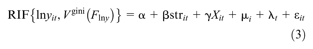
To analyze the impact of household structure on consumption inequality, we employ the Recentered Influence Function (RIF) regression of Firpo et al. (2009). Specifically, we estimate RIF regressions with respect to the Gini coefficient, which capture unconditional marginal effects of household structural types on inequality. This approach allows us to assess distributional impacts beyond the mean while controlling for household and time fixed effects. Formally, the model is specified as follows:

$$\mathrm{RIF}\{\ln c_{\mathrm{it}},V^{\mathrm{gini}}\left(F_{1\mathrm{n}c}\right)\}=\mathrm{\alpha }+\mathrm{\beta }\mathrm{st}{\mathrm{r}}_{\mathrm{it}}+\mathrm{\gamma }{X}_{\mathrm{it}}+{\mathrm{\mu }}_i+{\mathrm{\lambda }}_t+{\mathrm{\epsilon }}_{\mathrm{it}}$$

(1)

where $\mathrm{RIF}\{\ln c_{\mathrm{it}},V^{\mathrm{gini}}\left(F_{1\mathrm{n}c}\right)\}$ denotes the RIF-transformed outcome of log per capita consumption for household i in year t, with respect to the inequality statistic $\left(V\left(F_{1\mathrm{n}c}\right)\right)$ . The key explanatory variable, str _it , captures household structure and is operationalized as a set of dummy variables, with the nuclear household with children serving as the benchmark category. The control vector X_it includes household head characteristics (age, gender, marital status, education), household-level attributes (proportion of children, proportion of elderly, household size, log per capita income, log per capita wealth), and regional-level factors (urban–rural residence, provincial per capita GDP, and the urbanization rate). Household fixed effects (μ _i ) absorb time-invariant unobserved heterogeneity, while year fixed effects (λ _t ) capture common temporal shocks. The coefficient vector β identifies the unconditional marginal effects of alternative household structures, relative to the reference group, on the selected consumption inequality measure. In essence, β quantifies how shifts in household composition contribute to the distributional dynamics of consumption, after accounting for observed covariates and fixed effects (Appendix).

Influence Mechanism Test Model Setting

Building on the benchmark model and theoretical mechanism analysis, the following models are constructed to examine the transmission channels:

$$\mathrm{RIF}\{\ln w_{\mathrm{it}},V^{\mathrm{gini}}\left(F_{\ln w}\right)\}=\mathrm{\alpha }+\mathrm{\beta }\mathrm{st}{\mathrm{r}}_{\mathrm{it}}+\mathrm{\gamma }{X}_{\mathrm{it}}+{\mathrm{\mu }}_i+{\mathrm{\lambda }}_t+{\mathrm{\epsilon }}_{\mathrm{it}}$$

(2)

$$\mathrm{RIF}\{\ln y_{\mathrm{it}},V^{\mathrm{gini}}\left(F_{\ln y}\right)\}=\mathrm{\alpha }+\mathrm{\beta }\mathrm{st}{\mathrm{r}}_{\mathrm{it}}+\mathrm{\gamma }{X}_{\mathrm{it}}+{\mathrm{\mu }}_i+{\mathrm{\lambda }}_t+{\mathrm{\epsilon }}_{\mathrm{it}}$$

(3)

$$\mathrm{RIF}\{\ln S_{\mathrm{it}},V^{\mathrm{gini}}\left(F_{\ln s}\right)\}=\mathrm{\alpha }+\mathrm{\beta }\mathrm{st}{\mathrm{r}}_{\mathrm{it}}+\mathrm{\gamma }{X}_{\mathrm{it}}+{\mathrm{\mu }}_i+{\mathrm{\lambda }}_t+{\mathrm{\epsilon }}_{\mathrm{it}}$$

(4)

Where w_it represents the net worth per capita of the household i at time t, y_it is the net worth per income of the household i at time t, s_it is household saving rate.

Data Sources and Statistical Characteristics

The empirical analysis draws upon data from the China Family Panel Studies (CFPS), covering the survey waves conducted in 2012 to 2022.The China Family Panel Studies (CFPS) dataset, administered by the Institute of Social Science Survey at Peking University, consists of three modules: household, Adult, and Child. The Adult Module provides demographic information enabling precise classification of household structures, while the Family Module offers detailed economic data—including income, wealth, and consumption—essential for analyzing consumption inequality dynamics. The analysis focuses on households with heads aged 16 to 100 years. This sampling strategy is justified by two considerations: First is sample representativeness: households with heads younger than 16 or older than 100 are numerically minimal. Second is behavioral heterogeneity: excluded households (predominantly single-adult households due to unique circumstances) exhibit consumption patterns significantly diverging from the general population. Including such outliers risks overestimating consumption inequality. After excluding extreme and missing values, the final analytical sample comprises 35,671 observations.

The Dependent Variable

In the RIF regression framework proposed by Firpo et al. (2009), the dependent variable is constructed as the Recentered Influence Function (RIF) of the distributional statistic of interest. In this study, we focus on the Gini coefficient of household consumption inequality, and the dependent variable is therefore defined as RIF_Gini (lnci), where lnci denotes the logarithm of per capita household consumption for household i. A higher value of RIF_Gini indicates that the household lies further from the mean of the distribution and contributes more to inequality, while a lower value implies a smaller or even equalizing impact.

The Explanatory Variable

The explanatory variable is household structure. To classify household structures, intergenerational relationships are defined based on Wang and Wu (2019), with a minimum age gap of 20 years and a maximum gap of 45 years (due to fertility constraints). On this basis, building on Wang (2020) and Yang (2025), and considering China’s ongoing trends of household downsizing and population aging, this study classifies household structures into six categories: Lineal household, Extended/Complex household, Nuclear household with children, Couple-only nuclear household, Single-person household, and Other household. Specifically, (1) the Single-person household refers to a household in which the household head lives alone and independently without any co-resident household members. (2) The Extended/Complex household is defined as an enlarged multigenerational household composed of parents, two or more married children, and their grandchildren, reflecting a horizontally expanded, multi-nuclear structure that extends beyond a single parent–child unit. (3) The nuclear household with children consists of a married couple and their unmarried children, representing a standard two-generation core structure typical of the mid-family life cycle. (4) The Couple-only nuclear household includes only the couple (married partners), commonly observed during the “empty-nest” stage when adult children have left the parental home. (5) The lineal household refers to a vertically extended multigenerational household centered on direct parent–child or grandparent–grandchild relationships. (6) The other household category includes non-typical household arrangements not captured by the above five classifications, such as sibling households, mixed-marital-status households, or households with divorced/widowed adult children. The categorical household structures is operationalized as a set of dummy variables, with the nuclear household with children serving as the benchmark category.

Control Variables

The control variables are categorized into three groups: household-level characteristics, household head characteristics, and regional-level characteristics.

Firstly, household-level characteristics: (1) Proportion of elderly members (Uo): measured by the ratio of household members aged 60 and above to total household members. (2) Proportion of children (Uy): defined as the share of household members aged 14 or below in total household size. (3) Log of per capita net income (lny): household net income includes wage income, business income, property income, and transfer income. (4) Household size (familysize): measured by the total number of household members. (5) Log of per capita assets (lnw): household assets comprise housing, financial assets, and other major forms of wealth.

Secondly, household head characteristics: (1) Gender (gender): equals 1 if male, and 0 if female. (2) Marital status (marital): equals 1 if married, and 0 otherwise. (3) Education level (edu): categorized as follows: illiterate/semi-illiterate = 1; primary school = 2; junior high school = 3; senior high school/vocational/technical secondary school = 4; junior college = 5; bachelor’s degree = 6; master’s degree = 7; 8 = doctoral degree = 8. (4) Age (age): measured as the age of the household head.

Thirdly, Regional-level characteristics: (1) Urban residence (urban): equals 1 if the household is located in an urban area, and 0 if in a rural area. (2) Log of provincial per capita GDP (lngdp): reflects the level of economic development of the province where the household resides. (3) Provincial urbanization rate (cityratio): measured as the ratio of urban population to total provincial population.

Descriptive statistics of all variables are presented in Table 1. The results indicate that Households with children (fam5) and lineal households (fam6) account for the largest proportions, at 29.86% and 26.76%, respectively. This indicates that intergenerational co-residence remains prevalent under the joint influence of traditional family culture and intergenerational support obligations. Couple-only nuclear households (fam4) represent 19.17% of the sample, suggesting that with the intensification of low fertility and rising living costs, an increasing number of households are evolving toward smaller, two-person structures, reflecting stronger independence and a gradual shift away from extended family living. Single-person households (fam2) and other household types (fam1) account for 10.65% and 11.67%, respectively. Although their shares are relatively modest, they highlight a growing trend toward singularization, nontraditional forms, and diversification, driven by changing marriage norms, enhanced urban mobility, and broader lifestyle choices. This transformation signifies a gradual move away from marriage- and child-centered household structures toward more pluralistic living arrangements. In contrast, extended/complex households (fam3) comprise only 1.89%, indicating that large multigenerational or multi-branch households have become relatively rare in modern society—a pattern closely associated with urban housing constraints and the younger generation’s pursuit of independent living. So, these findings reveal that Chinese households structures are undergoing a profound transition—from traditional multigenerational co-residence to smaller, more nuclear, and diversified forms. This structural evolution reflects broader demographic and social transformations and provides an important context for understanding how household changes may shape patterns of consumption inequality.

Table 1.

Variable Descriptive Statistics.

Variable	Definition	Mean	SD	Min	Max
fam1	Other household	.1167	.3211	0	1
fam2	Single-person household	.1065	.3085	0	1
fam3	Extended/complex household	.0189	.1361	0	1
fam4	Couple-only nuclear household	.1917	.3937	0	1
fam5	Nuclear household with children	.2986	.4576	0	1
fam6	Lineal household	.2676	.4427	0	1
RIF_Gini	Recentered influence function value of the Gini coefficient based on log per capita consumption	.0546	.5758	−.7873	1.4978
age	Age of household head	50.4937	13.8207	16	96
gender	Gender of household head	.6191	.4856	0	1
urban	Urban dummy	.5077	.4999	0	1
marital	Marital status of household head	2.0654	.7974	1	5
edu	Educational attainment of household head	2.8562	1.4837	1	8
lnc	Log of per capita consumption	9.3334	.9909	3.434	14.6245
lny	Log of per capita income	9.4662	1.2752	0	16.0302
lnw	Log of per capita wealth/assets	10.8375	1.7516	0	21.4965
familysize	Household size	2.7674	1.3127	1	12
Uy	Proportion of young dependents (0–14)	.0142	.0648	0	.6667
Uo	Proportion of elderly dependents (65+)	.1751	.3195	0	1
cityratio	Urbanization rate	.5859	.1303	.3157	.8933
lngdp	Log of per capita GDP	10.8139	.444	9.8889	12.1564

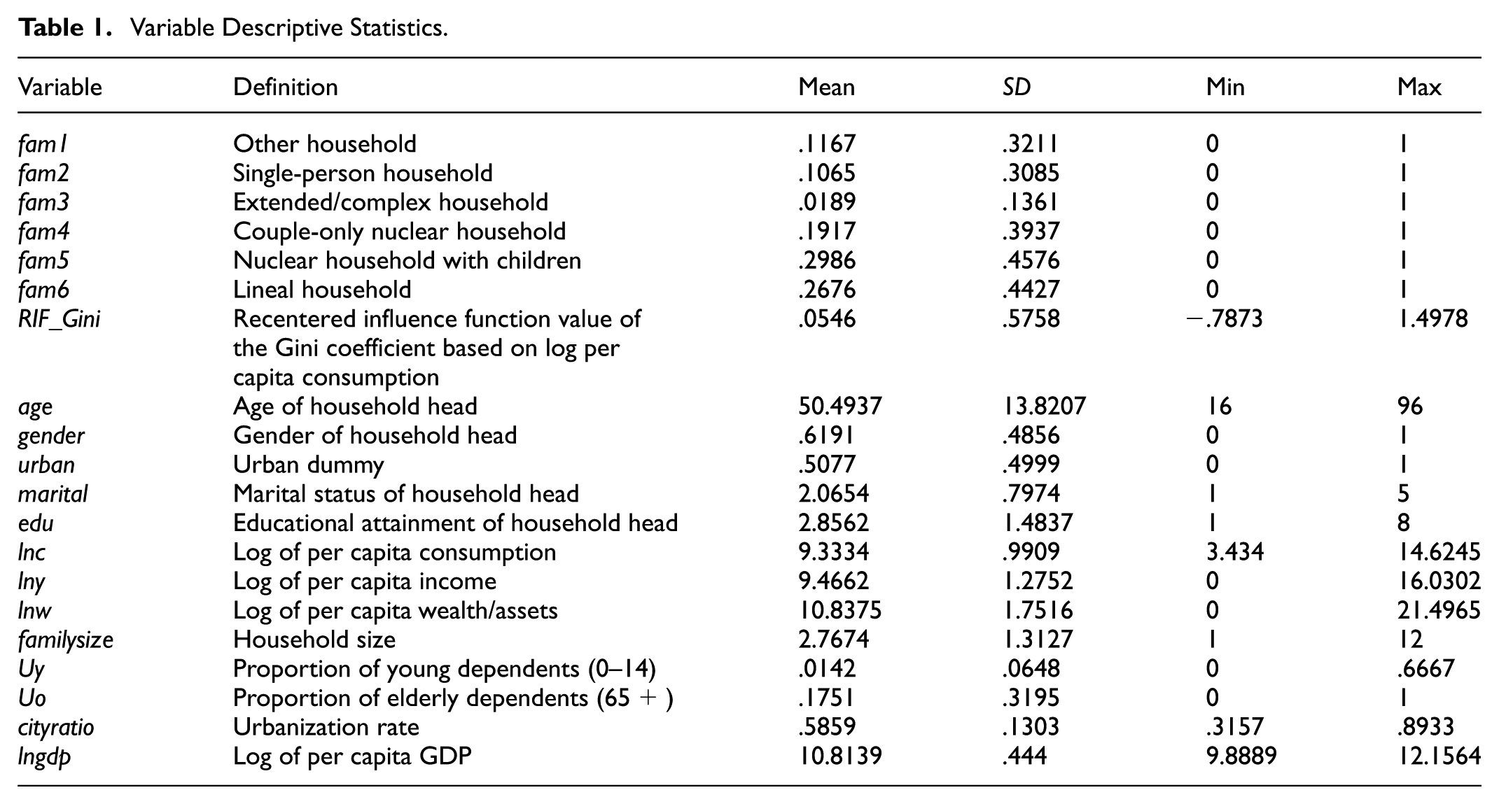
Moreover, the Recentered Influence Function value of the Gini coefficient (RIF_Gini) has a mean of .0546, indicating that the overall level of consumption inequality in the sample is relatively low, with only modest differences in consumption across households. However, the standard deviation of .5758 suggests substantial variation in households’ marginal contributions to overall inequality. In other words, although the average level of consumption inequality is low, households differ considerably in the extent to which they intensify or mitigate inequality within the overall consumption distribution.

Empirical Results

Baseline Regression

Table 2 reports the baseline regression results on the impact of household structure changes on consumption inequality. Column (1) presents the estimates without any control variables, while Columns (2) and (3) sequentially incorporate household-level, household-head-level, and regional-level controls. All regressions account for both time fixed effects and household fixed effects, which effectively mitigate two sources of potential bias: (1) omitted-variable bias arising from unobserved but time-invariant household characteristics that are correlated with consumption inequality, and (2) systematic shocks that are common to all households but unrelated to individual-specific traits. This empirical specification substantially enhances the reliability and precision of the estimated coefficients.

Table 2.

Baseline Regression Results.

	RIF–Gini (lnc)	RIF–Gini (lnc)	RIF–Gini (lnc)	RIF–Gini (lnc)
Variables	(1)	(2)	(3)	(4)
fam1	.0127*** (.0016)	.0128*** (.0016)	.3765*** (.0542)	.0125*** (.0016)
fam2	.0340*** (.0020)	.0310*** (.0021)	1.1245*** (.0738)	.0308*** (.0021)
fam3	.0231*** (.0038)	.0233*** (.0038)	.6520*** (.1211)	.0228*** (.0038)
fam4	.0093*** (.0015)	.0074*** (.0015)	.2541*** (.0535)	.0076*** (.0015)
fam6	.0080*** (.0013)	.0078*** (.0014)	.2188*** (.0450)	.0078*** (.0013)
Uy		−.0238*** (.0055)	−.7363*** (.1746)	−.0218*** (.0055)
Uo		−.0005 (.0021)	−.0246 (.0699)	−.0013 (.0020)
familysize		−.0003 (.0005)	−.01 (.0154)	−.0004 (.0005)
lny		.0020*** (.0005)	.1008*** (.0178)	.0020*** (.0005)
lnw		.0003 (.0004)	.0286** (.0134)	.0002 (.0004)
gender			−.0593* (.0308)	−.0016* (.0009)
edu			.0819*** (.0174)	.0022*** (.0005)
marital			.0084 (.0311)	.0003 (.0009)
age			.0017 (.0019)	.0001* (.0001)
cityratio				−.1436*** (.0170)
lngdp				.0215*** (.0032)
urban				.002 (.0018)
Time FE	Yes	Yes	Yes	Yes
Household FE	Yes	Yes	Yes	Yes
Constant	.0537*** (.0009)	.0343*** (.0059)	−.6928*** (.2366)	−.1249*** (.0310)
N	35,671	35,671	35,671	35,671
R 2	.5128	.5144	.5145	.5194

Notes. Robust standard errors clustered at the household level are reported in parentheses. The calculation results are rounded-up to three digits after the decimal point.

***

, **, and * indicates the level of significance of 1%, 5%, and 10%, respectively.

The results show that as additional controls are introduced, the signs and significance levels of the coefficients for household structure dummies remain stable. The coefficients of the core explanatory variables are consistently positive and statistically significant at the 1% level, indicating that—relative to nuclear households with children—other types of households (including other, single-person, compound, couple-only nuclear, and lineal households) exhibit significantly higher levels of consumption inequality. This finding supports Hypothesis 1, suggesting that when a household transitions from a nuclear-with-children structure to any other form, its degree of consumption inequality increases significantly.

This pattern reflects substantial differences across household types in terms of life-cycle stages, income stability, and risk-sharing capacity. Nuclear households with children are generally in the middle stage of the life cycle, characterized by stable income sources, dual labor participation, and stronger inter-temporal consumption-smoothing capacity. These features enable them to better withstand income shocks and maintain a relatively even level of consumption. In contrast, other household types—often located at earlier or later stages of the life cycle, or lacking intra-household risk-sharing mechanisms—are more vulnerable to income fluctuations, leading to greater disparities in consumption.

Specifically, the coefficients for single-person households (fam2), compound households (fam3), and other household types (fam1) are relatively large, implying that these households contribute more to overall consumption inequality. Single-person households lack income pooling and internal risk-sharing, causing their consumption to fluctuate sharply with income changes. In compound households, intergenerational differences in consumption preferences and resource allocation goals may generate intra-household imbalances and amplify cross-household disparities. Other nontraditional households (such as remarried or non-kin cohabiting households) face institutional disadvantages in social security and resource integration, further exacerbating inequality. By contrast, couple-only nuclear households (fam4) and lineal households (fam6) show smaller coefficients, suggesting that although their inequality levels exceed those of nuclear-with-children households, their relatively stable structure and more homogeneous consumption patterns help constrain the extent of inequality expansion.

Building on the analysis of overall consumption inequality, this study further examines how different household structures contribute to inequality across major consumption categories. The results are presented in Table 3.

Table 3.

Household Structure Change and Inequality of Different Consumption.

	RIF–Gini (lnfood)	RIF–Gini (lndrss)	RIF–Gini (lnhouse)	RIF–Gini (lndaily)	RIF–Gini (lnmed)	RIF–Gini (lntrco)	RIF–Gini (lneec)	RIF–Gini (lnother)
Variables	(1)	(2)	(3)	(4)	(5)	(6)	(7)	(8)
fam1	−.0021 (.0026)	−.0001 (.0066)	−.0008 (.0041)	.0019 (.0049)	−.0323*** (.0100)	−.005 (.0039)	.0375*** (.0133)	.0059 (.0119)
fam2	.0253*** (.0035)	.0372*** (.0081)	.0503*** (.0060)	.0278*** (.0058)	.0193 (.0126)	.0348*** (.0051)	.0633*** (.0150)	.0475*** (.0130)
fam3	−.0017 (.0051)	.0118 (.0120)	.0009 (.0081)	−.0039 (.0093)	−.0389** (.0195)	−.003 (.0077)	−.0075 (.0281)	.0168 (.0259)
fam4	.0031 (.0029)	.0250*** (.0070)	.0130*** (.0045)	.0136*** (.0048)	−.0212** (.0102)	.0133*** (.0039)	.0364*** (.0128)	.0123 (.0106)
fam6	−.0021 (.0023)	−.0088 (.0054)	.0005 (.0037)	−.0024 (.0041)	−.0238*** (.0091)	−.0031 (.0033)	−.0320*** (.0112)	−.0098 (.0099)
Control variables	Yes	Yes	Yes	Yes	Yes	Yes	Yes	Yes
Time FE	Yes	Yes	Yes	Yes	Yes	Yes	Yes	Yes
Household FE	Yes	Yes	Yes	Yes	Yes	Yes	Yes	Yes
Constant	−.0841 (.0564)	.0061 (.1402)	−.2722*** (.0922)	−.1906** (.0937)	.3498 (.2204)	−.0577 (.0800)	.6361** (.2619)	1.5843*** (.2326)
N	35,671	35,671	35,671	35,671	35,671	35,671	35,671	35,671
R 2	.4784	.576	.489	.4855	.4783	.6407	.6474	.5767

Notes. Robust standard errors clustered at the household level are reported in parentheses. The calculation results are rounded-up to three digits after the decimal point.

***

and ** indicates the level of significance of 1% and 5% respectively.

First, single-person households show consistently positive and statistically significant coefficients across nearly all eight categories, indicating that their consumption inequality is generally higher than that of nuclear households with children. This pattern may be explained by two factors. On one hand, single-person households rely heavily on individual income and lack intra-household income pooling and risk-sharing mechanisms, making their consumption more sensitive to income fluctuations. On the other hand, their expenditure choices tend to be more individualized and preference-driven, leading to greater heterogeneity in consumption behavior.

Second, couple-only nuclear households exhibit positive and significant coefficients in all categories except for food and miscellaneous spending, suggesting higher inequality in non-food consumption compared with nuclear households with children. This is primarily because, in the absence of childrearing responsibilities, couples display higher marginal propensities to consume, and differences in income and wealth are more clearly reflected in discretionary and improvement-oriented spending. Moreover, without the budgetary constraints or scale economies associated with children, these households have weaker consumption-smoothing capacity.

Third, compound households show a significantly negative coefficient only in health expenditure. This result can be attributed to the fact that multi-generational co-residence and diversified income sources strengthen intergenerational transfers and shared health spending mechanisms, which help smooth medical expenditures across household members and thereby reduce inequality in this category.

Fourth, lineal households and other nontraditional household types display significantly negative coefficients in both health care and transportation-communication expenditures, while showing weaker or insignificant effects in other categories. This pattern reflects the reality that in China, lineal households—typically consisting of two or three generations—tend to share medical, mobility, and communication resources, while nontraditional households (such as remarried or cohabiting households) often engage in joint consumption or cost-sharing arrangements. As a result, their spending on these shared or necessity-oriented categories is relatively even, leading to lower inequality in these dimensions.

Robustness Test

Alternative Dependent Variables

This study first conducts a robustness test by replacing the dependent variable. The baseline dependent variable is replaced with RIF–Var(lnc) and RIF–Iqr(lnc). Specifically, RIF–Var(lnc) reflects the overall dispersion of household consumption and captures the influence of extreme values on inequality, whereas RIF–Iqr(lnc) focuses on the interquartile range around the median, emphasizing inequality within the middle of the distribution.

The results in Table 4 show that the coefficients of the core explanatory variables remain significantly positive at the 1% level, consistent with the baseline regression results, thereby providing further support for Hypothesis 1.

Table 4.

Robustness Test: Alternative Dependent Variables.

	RIF–Var (lnc)	RIF–Iqr (lnc)
Variables	(1)	(2)
fam1	.3772*** (.0540)	.5029*** (.0824)
fam2	1.1273*** (.0736)	1.4644*** (.1061)
fam3	.6521*** (.1212)	.7383*** (.1893)
fam4	.2644*** (.0531)	.4261*** (.0818)
fam6	.2218*** (.0448)	.2713*** (.0702)
Control variables	Yes	Yes
Time FE	Yes	Yes
Household FE	Yes	Yes
Province FE	No	No
Constant	−6.2900*** (1.0982)	−5.6519*** (1.6293)
N	35,671	35,671
R 2	.5179	.4791

Notes. Robust standard errors clustered at the household level are reported in parentheses. The calculation results are rounded-up to three digits after the decimal point.

***

indicates the level of significance of 1%.

Alternative the Core Explanatory Variable

To further verify the robustness of the baseline regression results, this study conducts an additional robustness test by replacing the core explanatory variable. First, following the approach of Attanasio and Pistaferri (2016), Luo and Chen (2020), household structure is treated as a continuous pseudo-variable ranging from 1 to 6, representing variations across different types of household structures.

Second, to capture the dynamic aspect of household structure, we introduce a binary variable any change based on whether a household experienced structural transformation during the observation period (2012–2022). Specifically, households that underwent any change in structure are assigned a value of 1, whereas those maintaining the same structure throughout the period are coded as 0. This indicator helps to identify the impact of structural transitions on consumption inequality from a temporal perspective, thereby providing an additional robustness check.

Table 5 presents the regression results obtained after replacing the core explanatory variable. Columns (1) and (2) respectively report the estimation results using the ordered pseudo-variable and the structural-change dummy as alternative measures of household structure. The coefficients of the core explanatory variable remain significantly positive at the 1% level, and their signs and magnitudes are consistent with those of the baseline model. These findings confirm the robustness of the main conclusion.

Table 5.

Robustness Test: Alternative the Core Explanatory Variable.

	RIF–Gini (lnc)	RIF–Gini (lnc)
Variables	(1)	(2)
famtype	−.0032*** (.0003)
change		.1433*** (.0180)
Control variables	Yes	Yes
Time FE	Yes	Yes
Household FE	Yes	Yes
Constant	−.1065*** (.0314)	−3.5944*** (.4687)
N	35,671	35,671
R 2	.5103	.0392

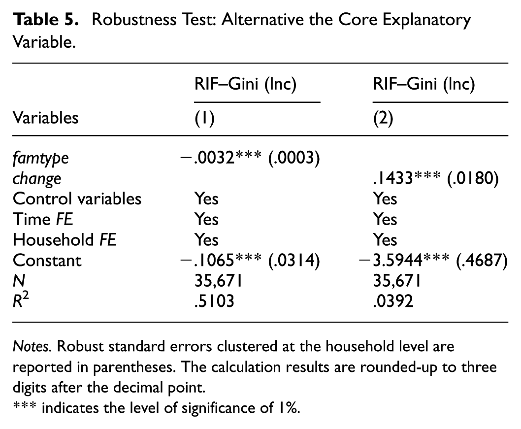
Notes. Robust standard errors clustered at the household level are reported in parentheses. The calculation results are rounded-up to three digits after the decimal point.

***

indicates the level of significance of 1%.

Adjusting Sample Size

Considering the potential influence of extreme observations and major external shocks on consumption inequality, we further adjust the regression sample in several ways to ensure the robustness of our findings. Table 6 reports the robustness check results based on different sample adjustments. Column (1) presents the estimation results after winsorizing all variables at the 1% and 99% levels to mitigate the impact of outliers. Column (2) excludes observations from 2018 onward to remove the potential interference of the U.S.–China trade frictions, while Column (3) further excludes the years after 2020 to account for the effects of the COVID-19 pandemic.

Table 6.

Robustness Test: Adjusting Sample Size.

	RIF_Gini	RIF_Gini	RIF_Gini
Variables	(1)	(2)	(3)
fam1	.0094*** (.0015)	.0092*** (.0029)	.0112*** (.0023)
fam2	.0219*** (.0019)	.0264*** (.0058)	.0373*** (.0035)
fam3	.0191*** (.0037)	.0137** (.0059)	.0175*** (.0049)
fam4	.0061*** (.0014)	.0077** (.0038)	.0092*** (.0024)
fam6	.0067*** (.0013)	.0076*** (.0027)	.0070*** (.0020)
Control variables	Yes	Yes	Yes
Time FE	Yes	Yes	Yes
Household FE	Yes	Yes	Yes
Constant	−.0372 (.0285)	−.0105 (.0506)	−.1579*** (.0440)
N	32,427	22,998	27,247
R 2	.5100	.636	.5834

Notes. Robust standard errors clustered at the household level are reported in parentheses. The calculation results are rounded-up to three digits after the decimal point.

***

and ** indicates the level of significance of 1% and 5% respectively.

Across all three specifications, the coefficients of the core explanatory variable remain significantly positive at the 1% level, indicating that the estimated relationship between household structural changes and consumption inequality is highly robust. These results reinforce the credibility of the baseline findings and provide additional support for Hypothesis 1.

Endogeneity Treatment

Using Lagged Explanatory Variables

To further address potential endogeneity arising from reverse causality, we regress the current dependent variable on the lagged values of all explanatory variables. This approach helps mitigate the bias caused by possible bidirectional causation between household structure and consumption inequality. Column (1) of Table 7 reports the estimation results using lagged explanatory variables. The coefficients of the core explanatory variable remain significantly positive at the 1% level, indicating that the issue of reverse causality has been effectively alleviated and that Hypothesis 1 is once again supported.

Table 7.

Endogeneity Treatment: Using Lagged Explanatory Variables and Adding Extended Controls.

	RIF–Gini	RIF_Gini
Variables	(1)	(2)
fam1	.0075*** (.0013)	.0124*** (.0020)
fam2	.0143*** (.0021)	.0256*** (.0023)
fam3	.0097*** (.0027)	.0205*** (.0045)
fam4	.0029** (.0013)	.0066*** (.0017)
fam6	.0032*** (.0010)	.0070*** (.0016)
Control variables	Yes	Yes
Time FE	Yes	Yes
Household FE	Yes	Yes
Constant	−.0350* (.0197)	.2135*** (.0474)
N	15,213	27,438
R 2	.0317	.5909

Notes. Robust standard errors clustered at the household level are reported in parentheses. The calculation results are rounded-up to three digits after the decimal point.

***

, **, and * indicates the level of significance of 1%, 5%, and 10%, respectively.

Adding Extended Controls

To further address potential endogeneity bias caused by omitted variables, this study incorporates indicators of household participation in medical, pension, and unemployment insurance to control for differences in social protection coverage. In addition, province fixed effects are introduced to account for regional heterogeneity in economic development, welfare systems, and public expenditure.

Column (2) of Table 7 reports the estimation results. The coefficients of the core explanatory variable remain significantly positive at the 1% level across all model specifications, indicating that even after accounting for these factors, household structural changes continue to exert a robust and significant impact on consumption inequality.

Instrumental Variable Estimation

To address potential endogeneity, this study employs the instrumental variable (IV) approach and estimates the model using two-stage least squares (2SLS). Two demographic variables are selected as instruments: whether the household has at least one parent aged 60 or above, and the number of parents aged 60 or above. The rationale for selecting these instruments is as follows: First, the presence of parents aged 60 or above significantly influences household decisions regarding living arrangements, caregiving responsibilities, and resource allocation, such as promoting intergenerational cohabitation or household merging. These demographic shocks are primarily determined by natural longevity, are exogenous in nature, and do not directly affect consumption inequality. Second, the number of surviving parents reflects the intensity of intergenerational caregiving pressure: as the number increases, the household’s economic and emotional burdens rise, making transitions from nuclear to extended or multigenerational households more likely. After controlling for income, wealth, education, urban–rural status, and macroeconomic factors, these variables affect consumption inequality only through household structural changes, satisfying the relevance and exogeneity conditions for valid instruments.

Table 8 shows that the first-stage results confirm the strong relevance of the instrumental variables: the Kleibergen–Paap LM statistic rejects the null hypothesis of under-identification, indicating a significant correlation between the instruments and household structural change; the Kleibergen–Paap rk Wald F statistic exceeds the critical value of 10 proposed byStaiger and Stock (1997), suggesting that weak instrument bias is not a concern; meanwhile, the Cragg–Donald Wald F value is higher than the 10% maximal IV bias threshold set by Stock and Yogo (2005), further validating the strength of the instruments. Since the model is exactly identified, the Hansen J statistic equals zero, indicating that the instruments satisfy the exogeneity condition.

Table 8.

Endogeneity Treatment: Instrumental Variable Estimation.

	RIF_Gini	RIF_Gini
Variables	(1)	(2)
Household structural change	−.6960*** (.2269)	−.6196*** (.2208)
Control variables	Yes	Yes
Time FE	Yes	Yes
Household FE	Yes	Yes
Constant	−1.9271*** (.2198)	−1.9350*** (.2073)
N	27,497	27,497
R 2	.1177	.1892
Underidentification (Kleibergen–Paap LM)	19.604 (p = .000)	18.476 (p = .000)
Weak identification (Kleibergen–Paap rk Wald F)	19.885	32.058
Cragg–Donald Wald F	34.377	18.845
Hansen J (overidentification)	.000	.000

Notes. Robust standard errors clustered at the household level are reported in parentheses. The calculation results are rounded-up to three digits after the decimal point.

***

indicates the level of significance of 1%.

The second-stage estimation results show that the coefficients of the core explanatory variable are all statistically significant. Therefore, household structural change has a significant impact on consumption inequality, which is consistent with the findings of the baseline regression.

Difference-in-Differences (DID) Regression

To address potential endogeneity issues, this study employs a Difference-in-Differences (DID) approach for empirical analysis, using the implementation of China’s universal two-child policy in 2016 as an exogenous shock.

$$\mathrm{RIF}\_\mathrm{Gin}{i}_{\mathrm{it}}=\alpha +\beta (\mathrm{Trea}{t}_i*\mathrm{Pos}{t}_t)+\gamma X_{\mathrm{it}}+{\mu }_{\mathrm{i}}+{\lambda }_t+{\mathrm{\epsilon }}_{\mathrm{i}\mathrm{t}}$$

(5)

Formally, let Treat _i denote an indicator variable that equals 1 if household i experienced a structural change (treatment group) and 0 otherwise. The variable Post _t for the post-policy period after the implementation of the universal two-child policy in 2016, and 0 for the pre-policy period. The interaction term Treat _i  × Post _t constitutes the core Difference-in-Differences (DID) estimator, capturing the additional effect of household structural change on consumption inequality following the policy intervention. The coefficient of interest, β\betaβ, measures the causal impact of household structural change on consumption inequality.

To address potential endogeneity concerns arising from the violation of the parallel trends assumption, we augment the baseline DID specification by incorporating group-specific linear time trends, which allow treatment and control groups to follow distinct long-run trajectories prior to the policy shock. Column (1) of Table 9 reports the results. After controlling for heterogeneous linear trends, the coefficient on the key interaction term Treat × Post remains positive and statistically significant (.1092, p < .01), indicating that household structural change significantly increased consumption inequality following the implementation of the two-child policy. This finding suggests that the estimated causal effect is robust even under a relaxed version of the parallel trends assumption.

Table 9.

Endogeneity Treatment: DID Regression.

	RIF–Gini (lnc)	RIF–Gini (lnc)
Variables	(1)	(2)
Treat × Post	.1092*** (.0196)
Treat × Post_placebo		.0056 (.0150)
Control variables	Yes	Yes
Time FE	Yes	Yes
Household FE	Yes	Yes
Constant	−1.8176*** (.2412)	−1.7838*** (.2413)
N	35,671	35,671
R 2	.1909	.1899

Notes. Robust standard errors clustered at the household level are reported in parentheses. The calculation results are rounded-up to three digits after the decimal point.

***

indicates the level of significance of 1%.

Furthermore, we conduct a placebo test to verify the reliability of our identification strategy. Specifically, we artificially assign the policy intervention year to 2014, 2 years prior to the actual reform, and re-estimate the DID model. As shown in Column (2), the coefficient of the placebo interaction term Treat × Post_placebo is statistically insignificant, this indicates that under the fictitious policy shock, there is no significant difference between the treatment and control groups. This finding suggests that the estimated policy effect is not driven by other contemporaneous external factors or underlying trend differences, thereby further confirming the robustness of the baseline regression results and the validity of the identification strategy.

Heterogeneity Analysis

Heterogeneity Analysis: Urban Versus Rural

Given the substantial differences between urban and rural households in terms of income sources, employment opportunities, social security coverage, and consumption environments, it is essential to further examine urban–rural heterogeneity. Such analysis helps identify the differentiated effects of household structure changes on consumption inequality under varying socioeconomic contexts.

The heterogeneity analysis (shown in Table 10) reveals that, compared with rural households, the regression coefficients of most household structure types—except for couple-only nuclear households—are generally larger in the urban sample. This finding indicates that household structural differences exert a stronger amplifying effect on consumption inequality in urban areas. The primary reason lies in the more diversified income sources and more pronounced social stratification among urban households, where disparities in occupation, education, and social security coverage across different household structures are more easily translated into consumption gaps.

Table 10.

Heterogeneity Analysis: Urban Versus Rural.

	RIF–Gini (lnc)	RIF–Gini (lnc)
	Urban households	Rural households
Variables	(1)	(2)
fam1	.0125*** (.0026)	.0062*** (.0023)
fam2	.0285*** (.0028)	.0268*** (.0037)
fam3	.0318*** (.0059)	.0127*** (.0047)
fam4	.0058*** (.0021)	.0078*** (.0025)
fam6	.0076*** (.0019)	.0053** (.0021)
Control variables	Yes	Yes
Time FE	Yes	Yes
Household FE	Yes	Yes
Constant	−.1205*** (.0455)	.0057 (.0498)
N	18,109	17,562
R 2	.594	.5214

Notes. Robust standard errors clustered at the household level are reported in parentheses. The calculation results are rounded-up to three digits after the decimal point.

***

and ** indicates the level of significance of 1% and 5% respectively.

In contrast, the positive effect of couple-only nuclear households on consumption inequality is more pronounced in rural areas. This can be attributed to the fact that such households, lacking both childrearing responsibilities and intergenerational support, are more vulnerable to income disparities. Moreover, rural households typically face limited and volatile income sources, coupled with underdeveloped social security systems and weak mutual aid networks, which reduce their capacity to smooth consumption and thereby amplify inequality.

Heterogeneity Analysis: Social Security

Social security programs—such as pension and medical insurance—directly influence a household’s ability to cope with income fluctuations and expenditure risks. Accordingly, households with and without social security coverage differ significantly in their capacity for risk management and consumption smoothing. This study conducts a heterogeneity analysis from the perspective of social security to examine how household structural differences affect consumption inequality under varying levels of social protection. Specifically, households are grouped according to whether they are covered by medical insurance or pension insurance, and separate regressions are conducted. The results are presented in Table 11.

Table 11.

Heterogeneity Analysis: Social Security.

	RIF–Gini (lnc)	RIF–Gini (lnc)	RIF–Gini (lnc)	RIF–Gini (lnc)
	With medical insurance	Without medical insurance	With pension insurance	Without pension insurance
Variables	(1)	(2)	(3)	(4)
fam1	.0126*** (.0017)	.0246 (.0514)	.0128*** (.0021)	.0154 (.0171)
fam2	.0317*** (.0022)	−.003 (.0442)	.0301*** (.0026)	.016 (.0134)
fam3	.0220*** (.0038)	.1114 (.0797)	.0229*** (.0047)	.0476 (.0352)
fam4	.0080*** (.0016)	−.0107 (.0360)	.0083*** (.0019)	−.0039 (.0105)
fam6	.0077*** (.0014)	−.0084 (.0392)	.0071*** (.0017)	.013 (.0150)
Control variables	Yes	Yes	Yes	Yes
Time FE	Yes	Yes	Yes	Yes
Household FE	Yes	Yes	Yes	Yes
Constant	−.1169*** (.0318)	−.1378 (.8163)	−.1488*** (.0394)	.1437 (.3038)
N	34,289	887	26,551	2,867
R 2	.5259	.9588	.5846	.8833

Notes. Robust standard errors clustered at the household level are reported in parentheses. The calculation results are rounded-up to three digits after the decimal point.

***

indicates the level of significance of 1%.

Theoretically, households lacking social security rely primarily on intra- household risk-sharing mechanisms, which tend to amplify consumption disparities. By contrast, households with social security coverage benefit from both institutional protection and internal support networks, leading to smaller consumption gaps. However, the empirical results reveal an opposite pattern. The heterogeneity analysis indicates that, among households covered by medical and pension insurance, the regression coefficients for different household structure types are all significantly positive, whereas in the sample of households without social security coverage, structural differences are statistically insignificant. In other words, consumption inequality is greater among households with social security coverage, which is contrary to the theoretical expectation. A possible explanation is that, China’s social security system exhibits selectivity and stratification. Social security coverage is more extensive among urban, formally employed, and higher-income households, which already display substantial differences in income and wealth levels. Moreover, these households enjoy greater income stability and predictable expenditures, allowing for higher discretionary spending and more diverse consumption patterns—thereby making consumption disparities more visible. In contrast, households without social security coverage are largely concentrated in lower-income groups, where overall consumption levels are constrained and differences remain statistically insignificant.

Heterogeneity Analysis: Eastern, Central, and Western Regions

Significant disparities exist across China’s eastern, central, and western regions in terms of economic development levels, income distribution, social security coverage, and the provision of public services. These regional differences shape households’ risk-coping capacities and resource allocation mechanisms, leading to heterogeneous effects of household structure across regions. Identifying how changes in household structure influence consumption inequality in different regions thus provides valuable insights for formulating region-specific policy recommendations.

The sample is divided into three regional groups—eastern, central, and western—based on the household’s location, and separate empirical analyses are conducted for each group. The results are presented in Table 12. The findings indicate that: Firstly, in the eastern region, the coefficients for other households (fam1) and extended/complex households (fam3) are relatively larger, indicating that consumption inequality among complex or nontraditional household structures is more pronounced in economically developed areas. This is primarily because, in regions with a higher degree of marketization, members of these household types tend to exhibit greater economic independence and weaker resource integration, leading to a wider dispersion in income and consumption. In contrast, the coefficients for single-person, couple-only nuclear households, and lineal households are smaller in the eastern region, suggesting that more comprehensive social security systems and diversified consumption channels in developed areas help to mitigate household-level consumption disparities to some extent.

Table 12.

Heterogeneity Analysis: Eastern, Central, and Western Regions.

	RIF–Gini (lnc)	RIF–Gini (lnc)	RIF–Gini (lnc)
	Eastern region	Central region	Western region
Variables	(1)	(2)	(3)
fam1	.0135*** (.0027)	.0115*** (.0032)	.0097*** (.0026)
fam2	.0266*** (.0030)	.0348*** (.0046)	.0302*** (.0038)
fam3	.0269*** (.0070)	.0231*** (.0060)	.0175*** (.0066)
fam4	.0045** (.0022)	.0097*** (.0033)	.0089*** (.0029)
fam6	.0077*** (.0021)	.0098*** (.0028)	.0047** (.0023)
Control variables	Yes	Yes	Yes
Time FE	Yes	Yes	Yes
Household FE	Yes	Yes	Yes
Constant	−.0553 (.0522)	.1721 (.1523)	.0271 (.0740)
N	15,433	8,548	11,690
R 2	.5622	.5248	.5080

Notes. Robust standard errors clustered at the household level are reported in parentheses. The calculation results are rounded-up to three digits after the decimal point.

***

and ** indicates the level of significance of 1% and 5% respectively.

Secondly, in the central region, the coefficient for single-person households (fam2) is the largest, and the coefficients for single-person, couple-only nuclear households, and lineal households are all higher than those in other regions. This indicates that the amplifying effect of household structural changes on consumption inequality is most pronounced in the central region. This pattern primarily reflects the region’s distinct economic and institutional characteristics. The central region is undergoing a phase of industrial restructuring and urban–rural dualization, characterized by a relatively high share of informal employment and unstable income sources. Meanwhile, the social security system remains unevenly distributed, and substantial urban–rural disparities persist. Compared with the western region, the central region enjoys a higher level of economic development and a more diversified consumption structure, which further magnifies inequality across household types.

Specifically, the single-person household (fam2) exhibits the highest coefficient, reflecting the greater vulnerability of such households in the central labor market, where employment instability and income fluctuations are more common. Without internal risk-sharing mechanisms, their consumption disparities become more pronounced. Couple-only nuclear households (fam4), free from the financial constraints of childrearing or elderly support, base their consumption decisions primarily on disposable income and preferences; however, larger income gaps among middle- and high-income groups in the central region exacerbate consumption inequality. For lineal households, pronounced urban–rural disparities in pension and education systems, along with insufficient public support, lead to significant variation in intergenerational transfers and caregiving expenditures, thereby translating into greater overall consumption inequality.

Thirdly, in the western region, the coefficients for most household structure types are smaller than those in other regions. This can be attributed to the relatively limited social security coverage and the more homogeneous income structure in the west, which together constrain the degree of consumption differentiation across households. Nevertheless, single-person households (fam2) exert the most pronounced effect, suggesting that unequal income and resource distribution remains the primary source of consumption inequality in the western region.

Influence Mechanism

From a micro-level perspective, household structures are closely aligned with different stages of the life cycle (Gilly & Enis, 1982). Life cycle theory posits that income, wealth, and consumption propensity are the primary determinants of household consumption behavior. Building on this theoretical framework, this study further examines whether changes in household structure affect consumption inequality through disparities in income, wealth, and consumption propensity (proxied by household saving rates). Given the inverse relationship between consumption propensity and precautionary saving motives (Carroll, 1992), the household saving rate is employed as a proxy indicator of consumption propensity, and analyses are conducted from three dimensions: income, wealth, and savings.

As reported in Table 13, the RIF regression results indicate that most household structure types exhibit positive and significant coefficients in the income and wealth inequality regressions. This suggests that, compared with nuclear households with children, most other household types experience greater disparities in income and wealth distribution. Notably, however, extended/complex households (fam3) and lineal households (fam6) are not significant in the wealth inequality regression, implying that intergenerational co-residence and resource pooling can partially mitigate wealth disparities within these households.

Table 13.

Influence Mechanism.

	RIF–Gini (lny)	RIF–Gini (lnw)	RIF–Gini (lns)
Variables	(1)	(2)	(3)
fam1	.0194*** (.0025)	.0070*** (.0027)	−5.1591*** (1.7069)
fam2	.0313*** (.0031)	.0302*** (.0035)	13.7918*** (2.0435)
fam3	.0275*** (.0056)	.009 (.0059)	−10.3857*** (3.3667)
fam4	.0143*** (.0023)	.0084*** (.0027)	3.4590** (1.6927)
fam6	.0132*** (.0022)	.0025 (.0023)	−5.0417*** (1.5525)
Control variables	Yes	Yes	Yes
Time FE	Yes	Yes	Yes
Household FE	Yes	Yes	Yes
Constant	−.0641 (0.0493)	−.2139*** (.0602)	211.3672*** (33.3964)
N	35,671	35,671	30,411
R 2	.5212	.5581	.5549

Notes. Robust standard errors clustered at the household level are reported in parentheses. The calculation results are rounded-up to three digits after the decimal point.

***

and ** indicates the level of significance of 1% and 5% respectively.

Regarding savings inequality, the coefficients for other households (fam1), extended/complex households (fam3), and lineal households (fam6) are significantly negative, with the strongest negative effect observed for extended/complex households. This finding suggests that multi-generational or resource-sharing households possess stronger risk-sharing and consumption-smoothing capacities, thereby reducing disparities in savings distribution. In contrast, single-person households (fam2) and couple-only nuclear households (fam4) exhibit positive and significant coefficients, with the largest positive effect found for single-person households. This result reflects the fact that single-person households lack internal support or pooling mechanisms, leading to more heterogeneous saving behaviors and consequently amplifying overall consumption inequality.

In summary, these results confirm Hypothesis 2, demonstrating that changes in household structure influence consumption inequality through three interrelated channels: income, wealth, and savings. Among these, income and wealth disparities serve as the primary amplifiers of consumption inequality, while differences in savings distribution reveal substantial heterogeneity in risk-sharing capacity and consumption-smoothing mechanisms across household structures. This finding confirms Hypothesis 2 (H2).

Further Discussion

The benchmark RIF regression results reveal that household structure changes exert a significant impact on consumption inequality. However, this analysis captures only the static differences across household structure types and fails to uncover the underlying mechanisms driving the evolution of inequality over time. In other words, while the benchmark regression identifies whether household structure changes affect consumption inequality, it does not explain how and through which channels these effects unfold.

To further investigate the sources and pathways through which household structure changes contribute to the growth of consumption inequality, this study employs the RIF-based Oaxaca–Blinder decomposition method (RIF-OB). This approach decomposes the overall change in inequality into two components: the characteristic effect, which reflects the influence of shifts in household structure distribution (i.e., changes in the proportion of different household types), and the coefficient effect, which captures variations in consumption behavior and marginal impacts across household types.

By applying this decomposition, the study distinguishes the relative contributions of structural distributional changes and behavioral effect changes to the rise in consumption inequality. This enables a more nuanced identification of the dynamic mechanisms through which household structure changes shape inequality, thereby providing empirical evidence for understanding the evolution of China’s consumption inequality and informing policies aimed at structural and behavioral adjustments.

Table 14 reports the decomposition results of household structure changes on the growth of consumption inequality from 2012 to 2022. The results show that the total change in consumption inequality is significantly positive, indicating an overall widening of consumption disparities during this period. Among the components, the characteristic effect is negative while the coefficient effect is positive, suggesting that shifts in household structure distribution helped narrow inequality, whereas behavioral changes within different household types contributed to its increase. In other words, during China’s structural transformation, it is changes in consumption behavior, rather than demographic distribution alone, that have primarily driven the rise in consumption inequality.

Table 14.

Decomposition Method.

Variable	Structure effect Δ_explained	Coefficient effect Δ_unexplained	Total contribution (Δ)	Share within household-structure contribution
Overall effects	−.0035*** (.0010)	.0082*** (.0008)	.0047*** (.0009)
Household structure
Single-person household	−.0034*** (.0003)	−.0010*** (.0002)	−.0044***	58.7%
Extended/compound household	.0003* (.0002)	.0001 (.0001)	.0004	5.3%
Couple-only nuclear household	−.0006** (.0003)	−.0009*** (.0003)	−.0015***	20%
Lineal household	.0005*** (.0002)	−.0010* (.0006)	−.0005	6.7%
Other	.0014*** (.0004)	−.0007* (.0004)	.0007	9.3%

Notes. Robust standard errors clustered at the household level are reported in parentheses. The calculation results are rounded-up to three digits after the decimal point.

***

, **, and * indicates the level of significance of 1%, 5%, and 10%, respectively.

From the perspective of specific household structures: Firstly, for single-person households, both the characteristic and coefficient effects are negative and statistically significant, with an overall contribution of −.0044. This indicates that although single-person households exhibit greater inequality in cross-sectional terms, the increase in their population share, combined with convergence in intra-group disparities, has mitigated overall consumption inequality. The rising number of single-person households has increased the proportion of low-consumption groups, thereby diluting the influence of high-consumption households and exerting a balancing effect on inequality. Moreover, between 2012 and 2022, single-person households have become increasingly younger and more urbanized, leading to more homogeneous consumption preferences and lifestyles. At the same time, enhanced social assistance for vulnerable populations and expanded protection for low-income elderly living alone have further reduced consumption gaps within this group. Therefore, behavioral differences among single-person households have narrowed over time, resulting in a negative coefficient effect that reflects growing homogeneity in their consumption patterns.

Secondly, the extended household exhibits a significantly positive characteristic effect, while its coefficient effect is small and statistically insignificant, with an overall contribution of .0004. This suggests that the rising proportion of extended households has slightly widened overall consumption inequality. The main reason is that extended households include both middle- and high-income households that choose intergenerational cohabitation to achieve resource pooling, and low-income households that are compelled to live together due to economic constraints. This composition generates a distinct “dual-polarization” pattern in income distribution, thereby amplifying overall disparities as their population share increases. However, during 2012 to 2022, the internal consumption gap within extended households remained relatively stable, as expanding social security coverage and intergenerational support mechanisms helped mitigate within-group inequality, leading to an insignificant coefficient effect.

Thirdly, he couple-only nuclear household exhibits both a significantly negative characteristic effect and negative coefficient effect, with an overall contribution of −.0015, indicating that the increasing share of such households and their evolving consumption patterns have jointly helped alleviate overall consumption inequality. This outcome can be attributed to structural and behavioral changes during 2012 to 2022. As China’s economic structure upgraded and the labor market stabilized, income volatility declined, and household income sources became increasingly diversified. At the same time, the rising female labor participation rate contributed to the expansion of the middle-income group, leading to a more balanced distribution of couple-only households across the income spectrum. Moreover, with the rapid development of digital finance and the widespread availability of credit access, households at different income levels gained greater access to financial resources and consumer credit. This enhanced credit availability enabled lower-income households to smooth consumption, narrowing intra-group consumption disparities and resulting in a negative coefficient effect.

Fourthly, the lineal household exhibits a significantly positive characteristic effect and a significantly negative coefficient effect, with an overall contribution of −.0005. This indicates that, between 2012 and 2022, the rising share of lineal households has slightly widened overall consumption inequality at the structural level, while intra-group disparities have narrowed, exerting a mitigating influence on total inequality. Due to a combination of institutional and cultural factors, China continues to rely primarily on household-based elder care. As population aging has intensified, the number of lineal households has increased, encompassing both high-consumption urban households and low-consumption rural households. This “cohabitation with divergence” pattern of structural expansion has contributed to greater dispersion in overall consumption distribution. However, the negative coefficient effect suggests that intra-group inequality among lineal households has declined over the same period. This can be attributed to the growing diversification of household income sources, the expansion of social security coverage, and the broader accessibility of public services, all of which have helped narrow consumption gaps and promote greater convergence between urban and rural lineal households.

Lastly, the other household category shows a positive characteristic effect and a negative coefficient effect, resulting in a net positive contribution. This indicates that the rising proportion of non-typical households has, on the whole, widened overall consumption inequality, while narrowing intra-group disparities, which partially offsets the inequality-expanding impact. This pattern can be explained by the fact that such households exhibit substantial heterogeneity in economic foundations and social security coverage, so their increasing share contributes to a broader gap in overall consumption. However, as household consumption decisions have become more rational and access to public services has improved, the consumption gap within this group has gradually narrowed, reflecting an internal convergence effect.

Furthermore, analyzing the relative contributions within the household-structure dimension reveals that single-person households account for 58.7%, playing the dominant role in mitigating inequality, followed by couple-only households (20.0%). In contrast, extended/compound households and lineal households exert smaller effects, while other households moderately amplify disparities. These proportions highlight that structural and behavioral adjustments among small-sized households are the key forces shaping inequality dynamics.

Conclusions and Implications

Conclusions

This study examines how household structure changes affect consumption inequality within China’s ongoing economic and demographic transitions.

First, significant overall effect: The diversification of household structures has markedly intensified consumption inequality. Compared with “nuclear households with children,” single-person, couple-only nuclear, extended/compound, lineal, and other non-typical households exhibit larger consumption gaps, suggesting that household disintegration and diversification form key micro-foundations of rising inequality.

Second, varying effects across categories: Impacts differ notably by expenditure type. Household structure changes exert the strongest effects on developmental and enjoyment consumption (education, culture, housing, transportation), while effects on subsistence consumption (food) are minimal, indicating that structural differences mainly widen higher-level consumption disparities.

Third, clear transmission mechanisms: Household structure influences inequality through income, wealth, and savings. Income and wealth disparities are the main amplification channels, reflecting heterogeneity in earning capacity and asset accumulation. Savings differences capture variations in risk-sharing and consumption-smoothing. Single-person and couple-only nuclear households consistently amplify inequality through all three channels, while compound and lineal households mitigate some inequality via savings, reflecting internal sharing mechanisms.

Fourth, marked heterogeneity: Urban structural disparities amplify inequality more strongly due to higher stratification and polarization, while rural couple-only nuclear households face wider gaps from unstable income and weak protection. Among insured households, inequality effects are more pronounced, indicating institutional stratification. Regionally, the eastern region shows the highest inequality for other and compound households, the central region the strongest amplification, and in the west, overall inequality is lower though single-person effects remain salient.

Fifth, dynamic decomposition: From 2012 to 2022, rising inequality is mainly driven by behavioral effects (coefficient changes), while compositional changes in household structures play a mild equalizing role—suggesting inequality expansion stems more from behavioral divergence within household types than from structural shifts.

Policy Implications

Promote Inclusive Consumption Upgrading

Given the structural disparities in high-level consumption, a “structure-sensitive” policy is needed. Targeted support in education, housing, and transport can narrow gaps and allow all household types to share the benefits of upgrading. For example, tax deductions and childcare subsidies for households with children, and housing or transport assistance for nontraditional and vulnerable households.

Adopt Stratified and Regionally Coordinated Governance

Impacts differ across urban–rural, social security, and regional dimensions. Cities should enhance equity in education, employment, and housing; rural areas should expand pension, medical, and financial coverage. Flexible enrollment and differentiated contribution schemes should reduce institutional barriers, while eastern and central regions enhance public services and western regions focus on baseline protection.

Strengthen Redistribution Mechanisms

Single-person households and couple-only nuclear households amplify inequality through limited income diversity and weak risk-sharing. Extended/Compound and lineal households widen income and wealth gaps due to heavy intergenerational burdens and poor coordination but show mitigating effects through savings. Policies should foster intergenerational sharing and resource integration to reduce structural consumption disparities. Policies should expand income sources, strengthen social insurance, support caregiving and education, and enhance intergenerational cooperation to reduce structural inequality.

This study has limitations, as CFPS data lack granular indicators for digital, green, and experience-based consumption, and the China-focused analysis restricts cross-country generalizability. Future work should combine survey data with platform records or administrative sources to uncover inequality mechanisms in new consumption domains and employ cross-regional or international comparisons to assess institutional and cultural differences. Such extensions will enhance understanding of consumption inequality under demographic change and inform more inclusive consumption policies.