Sage Journals: Discover world-class research

Abstract

This study analysed the influence of income growth, energy use, and consumption of renewable energy on carbon dioxide emissions in the selected 24 OECD countries. Using balanced panel data from 1990 to 2016, the study examined the relationship of income, energy use, and consumption of renewable energy with CO₂ emissions. To address the issue of cross-sectional dependence stemming from unobserved common factors, given the trading relationships among these countries, we employed the cross-sectionally augmented ARDL (CS-ARDL) and cross-sectionally augmented Distributed Lag (CS-DL) models to investigate the linkages among the above variables. The study revealed a positive correlation between energy use and CO₂ emissions, and a negative correlation between renewable energy consumption and CO₂ emissions. However, the study found no evidence to support the Environmental Kuznets curve hypothesis. Energy use and renewable energy consumption were also found to be causally linked to CO₂ emissions based on the Dumitrescu-Hurlin non-Granger causality test. However, the inverted U-shaped relationship of income growth with CO₂ emissions does not exist in the sampled OECD countries. Therefore, it is not advisable for these OECD countries to be dependent on income growth for environmental sustainability. Rather, these OECD countries need to directly cut down CO₂ emissions through the use of clean and renewable energy sources, decreasing non-renewable energy use. Moreover, considering the Jevons’ Paradox and the ‘rebound effects’ of energy efficiency gains that may increase overall energy consumption, a comprehensive approach combining energy efficiency and renewable energy integration is essential for mitigating CO₂ emissions and promoting environmental sustainability in these OECD countries.

JEL Classification: Q430; Q560.

Plain language summary

Do Income and Renewable Energy Consumption Mitigate CO₂ Emissions and Contribute to Sustainable Development in the OECD countries?

The study revealed a positive correlation between energy use and CO₂ emissions, and a negative correlation between renewable energy consumption and CO₂ emissions. However, the study found no evidence to support the Environmental Kuznets curve hypothesis. Energy use and renewable energy consumption were also found to be causally linked to CO₂ emissions based on the Dumitrescu-Hurlin non-Granger causality test. However, the inverted U-shaped relationship of income growth with CO₂ emissions does not exist in the sampled OECD countries. Therefore, it is not advisable for these OECD countries to be dependent on income growth for environmental sustainability. Rather, these OECD countries need to directly cut down CO₂ emissions through the use of clean and renewable energy sources, decreasing non-renewable energy use. Moreover, considering the Jevons Paradox and the ‘rebound effects’ of energy efficiency gains that may increase overall energy consumption, a comprehensive approach combining energy efficiency and renewable energy integration is essential for mitigating CO₂ emissions and promoting environmental sustainability in these OECD countries.

Keywords

Income renewable energy consumption sustainable development cross-sectional dependence cointegration CS-DL model D-H granger non-causality

Introduction

Around the world, pollution in all its forms, primarily driven by human economic activities, jeopardises sustainable economic growth, particularly in developing countries where agriculture chiefly relies on rainfall due to an increase in infrequent and insufficient rainfall. The rising level of major global pollutants, including CO₂ emissions, a significant component of Greenhouse Gases (GHG), is likely to increasingly disrupt climatic conditions, with a significant adverse impact on food production and, thus, food security.

The idea that a higher level of economic development will increase environmental awareness and control helps to explain this shift in the income-environmental link in the later stage of development. Increased environmental protection spending will also make renewable energy and the adoption of clean technology more readily available. Additionally, economies evolve, transitioning from less polluting rural and primitive industrial economies to comparatively cleaner service economies (Arrow et al., 1995; Panayotou, 1993). In light of this, it is predicted that this will result in less environmental deterioration at a later stage of economic development.

The theory of the Environmental Kuznets Curve (EKC) provides a theoretical underpinning to investigate the relationship between economic growth and environmental degradation. The EKC concept aroused the interest of several researchers worldwide. It predicts that the relationship between a country’s economic development and environmental degradation is in the shape of an inverted U. This gives people optimism and faith that the declining environmental quality will stabilise and start to improve after economic development reaches a certain level.

As a result, there exists a sound theoretical support in favour of the inverted U-shaped correlation between economic progress and environmental quality. Both structural and behavioural elements may be involved in this relationship. The level of economic activity, the distribution of output across sectors, and technological advancements are examples of structural variables, whereas an example of a behavioural force (Grossman & Krueger, 1995; Kaufmann et al., 1998; Panayotou, 1993) is the income elasticity of demand for environmental quality. Consumers are likely to pay more for better environmental quality (Lekakis & Kousis, 2001; McConnell, 1997; Roca, 2003). As income rises, so does this desire. Transnational trade patterns, the migration of industrial activities, demographic considerations, and the distribution of family income are other factors that are believed to be implicated in this association (Heerink et al., 2001; Heil & Selden, 2001; Magnani, 2000; Shi, 2003).

The EKC theory inspires hope that economic progress and prosperity will continue sustainably after a slow climb and the attainment of a peak in environmental deterioration. Put another way, it assumes that having more money will inevitably lead to pressure to stop environmental damage. This appears improbable in light of the growing evidence of global warming, climate change, and the accompanying adverse economic consequences for the entire world community.

Numerous works of literature have endorsed the EKC theory (Apergis, 2016; Awaworyi Churchill et al., 2018; Bilgili et al., 2016; Chen, Wang, & Zhong, 2019; Dogan & Seker, 2016; Dong, Hochman et al., 2018; Lau et al., 2019; Shafiei & Salim, 2014; Sharif et al., 2019; Sinha & Shahbaz, 2018; Yao et al., 2019). Inglesi-Lotz & Dogan, 2018; Liu et al., 2017; Mikayilov et al., 2018; Vo et al., 2020; Zhang & Liu, 2019; Zoundi, 2017)

However, several other studies have found no evidence to support the EKC theory. Similarly, the conflicting findings on the connection between CO₂ emissions and renewable energy consumption are also found in another body of literature. A number of studies (Allard et al., 2018; Alvarez-Herranz et al., 2017; Anwar et al., 2021; Balsalobre-Lorente et al., 2018; Ben Jebli et al., 2020; Bilgili et al., 2016; Cai et al., 2018; Dogan & Seker, 2016; Dong, Sun et al., 2018; Inglesi-Lotz & Dogan, 2018; Liu et al., 2017; Ma et al., 2021; Shafiei & Salim, 2014; Sinha & Shahbaz, 2018; Vo et al., 2020; Yang et al., 2021; Yao et al., 2019; Zoundi, 2017) support a negative relationship between renewable energy consumption and emissions. However, some studies have also found either no relationship or a positive relationship between the use of renewable energy and CO₂ emissions (Apergis et al., 2010; Menyah & Wolde-Rufael, 2010). Rising economic activity and the utilisation of fossil fuels for energy consumption have been the main causes for the one-and-a-half-fold increase in greenhouse gas (GHG) emissions since 1990 (OECD, 2023).

Numerous studies have attempted to test the validity of the EKC theory predicting an inverted U-shaped connection between environmental deterioration and economic growth, using a range of data analytic methodologies. Most of them, however, are methodologically weak, particularly the studies whose analysis is based on panel data, and which typically do not deal with the issue of cross-sectional dependence. The parameter estimations become inconsistent when cross-sectional units are cross-sectionally dependent (Chudik & Pesaran, 2015; Ditzen, 2021). For calculated parameters to be consistent and dependable, cross-sectional dependence between panel data units must be taken into consideration.

The OECD countries have made little progress in reducing emissions, and due to the recent surge in energy use, GHG emissions are projected to rise further (OECD, 2023). According to the OECD data, 29% of all the GHG emissions in OECD countries are produced by the energy sector, with 24% coming from the transportation sector, 13% from manufacturing, 9% from agriculture, and 25% from other sectors. Despite the general consensus that the use and consumption of fossil fuels is the main source of CO₂ emissions, a number of prior studies have found that renewable energy sources generate less emissions than fossil fuels (Ahmed et al., 2017; Petinrin & Shaaban, 2015; Rana et al., 2016). One of the crucial factors driving the expansion of renewable energy sources is the need to increase energy production and consumption while preserving the environment. Renewable energy systems are typically thought to be less polluting than fossil fuels at the moment of use (Liu et al., 2017), despite the fact that they may have major environmental impacts at other phases of the system’s life cycle (Quek et al., 2018). The United Nations’ inclusion of affordable and clean energy as the seventh of its 17 Sustainable Development Goals underlines the important role of clean or green energy and renewable energy consumption in the sustainable development of all nations, including those in the OECD, as indicated by GHG emissions per capita indicate the relative contribution to global greenhouse gas emissions. OECD nations emit significantly more CO₂ per person than the majority of other global regions. In 2019, the average CO₂ emissions per person in OECD nations were 8.3 tonnes, whereas the global average was 4.4 tonnes (OECD, 2023). The sampled OECD countries are also high-income countries that are suitable for investigating the validity of the EKC hypothesis.

Because of their interconnected trade links, it is anticipated that the panel data on sampled OECD countries are likely to be cross-sectionally dependent. Therefore, it is essential to test and address the issue of cross-sectional dependency brought on by unobserved common factors to ensure the statistical validity of the estimated parameters of the model.

Examining how the use of energy, income growth and the consumption of renewable energy affect carbon dioxide emissions and their consequences for environmental sustainability in OECD countries is the main objective of this research. This study also considers the problem of cross-sectional dependency in the data set by choosing and applying a suitable econometric model to analyse the influence of energy use, income growth, and renewable energy consumption on carbon dioxide emissions.

Theoretical Underpinnings

The connection between energy use, economic growth, renewable energy, and emissions has been thoroughly studied in environmental economics, energy policy, and sustainability research. The following is a list of key theoretical concepts and frameworks that explain these processes:

The EKC Theory

The EKC theory postulates, especially in the context of CO₂ emissions, that there is an inverse U-shaped linkage between the level of income and environmental degradation in a country. According to this theory, in the early phase of economic development, industrialisation raises CO₂ emissions by increasing energy consumption, which is frequently sourced from fossil fuels. However, as an economy matures, technological advancements, structural shifts, and increased environmental awareness lead to a greater adoption of renewable energy, resulting in reduced emissions (Grossman & Krueger, 1995; Stern, 2004).

Energy Ladder Theory

This theory suggests that energy consumption transitions as societies develop. Lower-income populations rely on traditional biomass (e.g., wood and charcoal), which emits lower CO₂ per capita but is less efficient in terms of energy use. As incomes rise, households and industries increasingly adopt fossil fuels, leading to higher CO₂ emissions. With higher incomes and technological advancements, societies shift towards cleaner, renewable energy sources in later stages, leading to lower emissions (Hosier & Dowd, 1987).

Decoupling Theory

The decoupling theory focuses on the potential to separate economic growth from environmental degradation. It distinguishes the concept of relative decoupling from absolute decoupling. According to the theory of relative decoupling, CO₂ emissions increase more slowly than economic production because renewable energy sources and energy efficiency improvements are not being adopted as quickly. The absolute decoupling theory states that economic growth can occur while total CO₂ emissions decline. Often, this is accomplished by incorporating extensive renewable energy sources.

Energy Transition Theory

This theory focuses on the transition from fossil fuel-reliant energy systems to renewable energy systems for lowering CO₂ emissions. The transition is driven by technological innovation (e.g., advancements in solar, wind, and storage technologies). policy interventions (e.g., carbon pricing, subsidies for renewables) and social and market dynamics that favour cleaner energy sources (Smil, 2016).

Carbon Lock-In Theory

This theory explains how dependence on fossil fuel-based energy systems creates path dependencies, delaying the adoption of renewable energy and perpetuating high CO₂ emissions. Key mechanisms include infrastructure investments favouring fossil fuels, the fossil fuel industry’s political and economic power, and social inertia in energy consumption habits (Unruh, 2000).

Porter’s Hypothesis

This hypothesis suggests that stringent environmental regulations, such as promoting renewable energy, can stimulate innovation and efficiency, leading to reductions in CO₂ emissions without hindering economic growth (Porter & Linde, 1995).

Rebound Effect Theory

This theory highlights how improvements in energy efficiency or the adoption of renewables may not lead to proportional reductions in CO₂ emissions due to increased consumption resulting from cost savings (direct rebound) and indirect economic effects that stimulate growth and energy use (Sorrell, 2007).

Structural Change Theory

This theory explains how transitions from energy-intensive sectors (e.g., manufacturing) to service-oriented economies can lead to reduced CO₂ emissions. Renewable energy adoption accelerates this decoupling process by providing cleaner energy alternatives (Antweiler et al., 2001).

These theories provide a comprehensive framework for understanding the interaction among energy consumption, renewable energy adoption, and emissions.

Literature Review

This section examines the previous empirical research to test the economic hypotheses, its history and justification. Finally, the results of major empirical investigations are presented in tabular form.

Kuznets (1955) hypothesised a relationship between economic development and inequality. Kuznets’ theory states that economic inequality increases in the initial stage of economic development, reaches a peak, and thereafter starts to decline as the economy develops, resulting in an inverted U-shaped relationship between economic development and inequality, known as the Kuznets curve.

Grossman and Krueger (1991) adopted the concept of the Kuznets curve in their study to examine the environmental impact of the North American Free Trade Agreement (NAFTA). During their background research for the World Development Report, they again emphasised the EKC theory as described in Shafik and Bandyopadhya (1992).

The EKC theory explains that as wealth increases due to growing economic activity, it generates and raises the demand for improved environmental quality, encouraging investment, development, and the adoption of better technologies to enhance environmental quality. In most countries, accumulating wealth is the most efficient way to improve the environment, while economic growth frequently causes deterioration in the environment in the early stages of development (Beckerman, 1992). Studies on testing the EKC hypothesis have found evidence to support an inverted U-shaped association between environmental deterioration and income (Grossman & Krueger, 1991, 1995).

Mirza and Kanwal (2017), using the ARDL technique and cointegration analysis, found a two-way causality among energy consumption, income, and CO₂ emissions. Stern (1998) examined the knowledge development regarding the EKC and addressed the various critiques levied at some empirical findings and their justifications in the policy literature.

Using the GMM technique, a panel data analysis of 14 Asian countries from 1990 to 2011 revealed evidence supporting the EKC theory (Apergis & Ozturk, 2015). According to their study, CO₂ emissions and income have an inverted U-shaped relationship and hence supported the EKC theory. (Ben Jebli et al., 2016) examined the relationship between GDP and per capita CO₂ emissions for a panel of 25 OECD countries from 1980 to 2010. They applied both FMOLS and DOLS estimators. Their study also validated the EKC hypothesis for the OECD.

In an analysis of the impact of GDP, renewable energy, and fossil fuels on CO₂ emissions in 11 U.S. states using annual data from 1980 to 2015, the EKC hypothesis was shown to be valid only in Illinois, Michigan, Florida, New York, and Ohio (Işık et al., 2019). Furthermore, this study found that fossil fuel consumption in Texas had a negative correlation with CO₂ emissions, whereas energy use in Florida had a positive correlation.

Economic growth, energy consumption, and CO₂ emissions are all interconnected, and both aspects contribute to the country’s rising CO₂ emissions, according a study on Pakistan (Khan & Ozturk, 2020).

The EKC theory was tested in 12 selected East African countries for the period 1990 to 2013 (Demissew Beyene & Kotosz, 2020). The EKC theory was supported by the study’s findings, based on the data analysis using the pooled mean group (PMG) technique.

An overview of previous empirical studies on OECD and other nations is given in the table below. Using panel and time series data analysis, this study examined the relationships among income, energy use, consumption of renewable energy, and emissions (Table 1).

Table 1.

Empirical Studies on CO₂ Emissions and their Findings.

Studies	Sample	Period	Main Findings
Moomaw and Unruh (1997)	16 OECD countries	1950–1992	It supports the EKC hypothesis
Dijkgraaf and Vollebergh (2005)	24 OECD countries	1960–1997	It supports the EKC hypothesis
Galeotti et al. (2006)	28 OECD and 93 non-OECD countries	1960–1997 1971–1997	It supports the EKC hypothesis
Shafiei and Salim (2014)	OECD countries	1980–2011	Renewable energy consumption (REC) lowers emissions, whereas non-renewable energy consumption (NREC) raises them, supporting the EKC theory
Bilgili et al. (2016)	17 OECD countries	1977–2010	REC lowers CO₂ emissions, which validates the EKC theory
Apergis (2016)	15 OECD countries	1960–2013	It backs up the EKC theory
Ben Jebli et al. (2016)	25 OECD countries	1980–2010	It supports the EKC hypothesis
Alvarez-Herranz et al. (2017)	17 OECD countries	1990–2012	N-shaped EKC is supported, and REC lowers CO₂ emissions
Awaworyi Churchill et al. (2018)	OECD countries	1870–2014	It supports the EKC hypothesis
Lau et al. (2019)	18 OECD countries	1995–2015	It supports the EKC hypothesis. NREC leads to a rise in CO₂ emissions, but nuclear energy causes a fall in CO₂ emissions
Allard et al. (2018)	74 countries	1994–2012	Except for upper-middle-income nations, it supports the N-shaped EKC; REC lowers CO₂ emissions.
Balsalobre-Lorente et al. (2018)	Italy, Spain, Germany, France, UK	1985–2016	The N-shaped EKC is supported, and the REC lowers CO₂ emissions.
Awaworyi Churchill et al. (2018)	OECD countries	1870–2014	It supports the N-shaped EKC
Dong, Hochman et al. (2018)	128 countries, different geographical clusters	1990–2014	REC and economic expansion lower CO₂
Dong, Sun et al. (2018)	China	1993–2016	It backs up the nuclear energy EKC concept; REC lowers CO₂ emissions
Inglesi-Lotz and Dogan (2018)	Sub-Saharan countries	1980–2011	Since REC lowers CO₂ emissions and NREC raises them, it contradicts the EKC hypothesis.
Cai et al. (2018)	G7 countries	1965–2015	REC reduces CO₂ emissions in Germany and US
Mikayilov et al. (2018)	Azerbaijan	1992–2013	The EKC theory is not supported by it
Sinha and Shahbaz (2018)	India	1971–2015	It supports the EKC hypothesis, and REC reduces CO₂ emissions
Ulucak and Bilgili (2018)	Low-income, middle-income and high-income countries	1961–2013	It supports the EKC hypothesis
Wang et al. (2018)	170 countries	1980–2011	The results differ according to the countries’ levels of per capita income.
Charfeddine and Kahia (2019)	MENA countries	1980–2015	REC reduces emissions
Chen, Wang, and Zhong (2019)	China	1980–2014	REC lowers CO₂ emissions, validating the EKC theory.
Chen, Zhao et al. (2019)	Chinese regions	1995–2012	Regional differences exist in the effects of REC and NREC.
Yao et al. (2019)	17 countries	1990–2014	REC reduces CO₂ emissions; It supports the EKC hypothesis
Lau et al. (2019)	18 OECD countries	1995–2015	The EKC hypothesis is supported; nuclear energy lowers CO₂ emissions, whereas NREC raises them.
Zhang and Liu (2019)	10 Northeast and Southeast Asian countries	1995–2014	It does not support the EKC hypothesis. REC reduces emissions
Ben Jebli et al. (2020)	102 countries	1990–2015	REC increases CO₂ emissions
Vo et al. (2020)	Japan, Mexico, Malaysia, Australia, Canada, Chile, New Zealand, Peru	1971–2014	REC reduces CO₂ emissions
Anwar et al. (2021)	ASEAN nations (Malaysia, Thailand, Singapore, the Philippines, Vietnam, and Indonesia)	1980–2013	The EKC hypothesis is supported in different quantiles; REC reduces CO₂ emissions
Ma et al. (2021)	France, Germany	1995–2015	REC lowers CO₂ emissions, whereas NREC raises them, supporting the EKC.
Yang et al. (2021)	The Silk Road Economic Belt (SREB) initiatives include 24 nations.	1995–2014	NREC increases CO₂ emissions while REC decreases them, supporting the EKC hypothesis

Source. The authors.

Most of the prior research has shown that the relationship between GDP per capita and emissions is represented by an inverted U-shaped curve. The bulk of studies on this linkage carried out in OECD countries also corroborate the EKC theory. Previous empirical research has shown that using renewable energy lowers CO₂ emissions while using non-renewable energy raises them. However, the literature reviews cited above suggest that there are few studies on OECD countries examining the impact of renewable energy use on carbon dioxide emissions. Additionally, not many studies on OECD countries use a model that quantifies the influence of renewable energy sources and takes cross-sectional dependence into consideration.

The Cross-Sectionally Augmented Autoregressive Distributed Lag (CS-ARDL) model and the Cross-Sectionally Augmented Distributed Lag (CS-DL) model are two sophisticated econometric models chosen and estimated in this work to account for diverse dynamics and coefficients across units. These models are built to tackle the dynamic misspecifications and residual serial correlation. This study also examines the effects of the consumption of renewable energy, alongside income and energy use, after controlling for cross-sectional dependence in the OECD countries being studied.

Data and Model Specification

Since data on energy use and renewable energy consumption are available until 2016, we used a balanced panel of annual data of the 24 OECD countries over the period 1990 to 2016. The dependent variable is the log of CO₂ emissions per person. The explanatory variables are the log of real GDP per capita, the square of the log of real GDP per capita, the log of energy use per capita, and the log of renewable energy consumption per capita. The data on the above variables were compiled from the World Bank’s database on the World Development Indicators available on its website (www.worldbank.org).

The descriptions of the variables considered for the analysis are given below (Table 2).

Table 2.

Variables Description.

Variables	Unit	Variables in log
CO₂ emissions per capita	Kt	co2
GDP per capita	PPP at constant 2017 international $	y
Energy use per capita	Kg of oil equivalent	eu
Renewable energy consumption per capita	TJ	re

Source. The authors.

We estimate the following basic long-term relationships:

\begin{array}{l} c o 2_{i, t} = β_{0, i} + β_{1, i} y_{i, t} + β_{2, i} y_{i, t}^{2} \\ + β_{3, i} e u_{i, t} + β_{4, i} r e_{i, t} + u_{i, t} \end{array}

(1)

Where $β_{0, i}$ , $β_{1, i}$ , $β_{2, i}$ , $β_{3, i}$ and $β_{4, i}$ are parameters and $u_{i, t}$ , the error term.

Due to trade links among the studied countries and resulting unobserved common factors giving rise to the likely problem of cross-sectional dependence, we adopt the CS-ARDL (Chudik & Pesaran, 2015) and CS-DL (Chudik et al., 2016) estimate methods. Dahmani et al. (2023), Namahoro et al. (2021), Okumus et al. (2021), and Sohail et al. (2023) have also used these models in their studies.

We anticipate that the four explanatory variables’ coefficients in the equation above will have the following signs:

β_{1, i} > 0, β_{2, i} < 0, β_{3, i} > 0, a n d β_{4, i} < 0 .

The EKC hypothesis will be valid if $β_{1, i} > 0$ , and $β_{2, i} < 0$ , and they are also statistically significant. If $β_{3, i} > 0$ , and also statistically significant, it will support the energy-led environmental degradation hypothesis. If $β_{2, i} < 0$ , and also statistically significant, it will support the hypothesis of a renewable energy-led sustainable environment.

Results and Discussion

Cross-Sectional Dependence Test

Firstly, we ascertain whether the variables are cross-sectionally dependent. Following Pesaran (2015), we apply the CD test to check weak cross-sectional dependence in the panel data set. The test’s null hypothesis is that the variable is weakly cross-sectionally dependent. Below are the CD test results (Table 3).

Table 3.

Cross-Sectional Dependence Exponent (Alpha) Estimation and Test.

Variables	Alpha	Standard error
co2	0.8876	0.0414
y	1.0061	0.0503
y²	1.0061	0.1016
eu	0.9223	0.0512
re	0.9465	0.1888
Test of Weak Cross-sectional Dependence
Variables	CD-test statistic	p-value
co2	16.385*	0.000
y	76.507*	0.000
y²	76.407*	0.000
eu	25.207*	0.000
re	19.558*	0.000

Source. The authors.

Significant at 1%.

The null hypothesis that each variable has a weak cross-sectional dependency is rejected by the CD test. The estimated values of the cross-sectional dependence exponent (alpha) above 0.5 and about 1 imply strong cross-sectional dependence. Hence, we must choose and apply an estimation method that controls for the issue of the dataset’s cross-sectional dependence. The Common Correlated Effects approaches seek to remove cross-sectional dependence by including cross-sectional averages in the model. The cross-sectional averages are partially separated using this method. To address cross-sectional dependence, we lag each variable and then add the cross-sectional averages of the bases of all variables.

Slope Heterogeneity Test

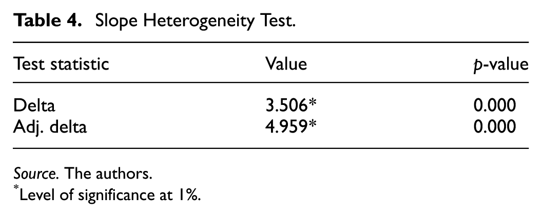
The panel data could be either homogeneous or heterogeneous. The choice of regression technique depends on whether the panel is homogeneous or heterogeneous. We apply the test for slope heterogeneity to ascertain whether the panel is homogeneous or heterogeneous. The p-values for both the delta and adjusted delta test statistics are significant at the 1% level. Thus, the test rejects the null hypothesis that the slopes are homogeneous and concludes that they are heterogeneous across the cross-sectional units (Table 4).

Table 4.

Slope Heterogeneity Test.

Test statistic	Value	p-value
Delta	3.506*	0.000
Adj. delta	4.959*	0.000

Source. The authors.

Level of significance at 1%.

Panel Unit Root Tests

Cross-sectional dependence among variables is confirmed, and the slope heterogeneity test indicates that the panel is also heterogeneous. The CIPS unit root tests (Pesaran, 2007) are considered to be appropriate for examining cross-sectional dependence in these circumstances. The null hypothesis of the CIPS test is that a variable is homogeneous and non-stationary, while the alternative hypothesis is heterogeneous and stationary.

The Cross-sectionally Augmented Dickey-Fuller (CADF) test (Pesaran, 2007) is another unit root test considered appropriate for variables showing cross-sectional dependence. It was also developed for the panel unit root test. The CADF test employs a t-test in the heterogeneous panels. The CADF test assumes that a variable is non-stationary under the null hypothesis. To remove the influence of cross-sectional dependence, the Dickey-Fuller or Augmented Dickey-Fuller regressions are supplemented by the cross-sectional averages of the lagged levels and the initial differences of individual variables.

The following table presents the results of the second-generation panel unit root test. As per the results of the CIPS and CADF tests, y, y², eu, and re are I(1), whereas co2 is I(0). These variables have a heterogeneous order of integration (Table 5).

Table 5.

Panel Unit Root Test.

Variables	CIPS-test	CADF-test
co2	−2.179**	−1.697
y	−1.976	−1.892
y²	−1.966	−1.913
eu	−1.924	−1.815
re	−1.875	−1.088
D(co2)	−4.792*	−2.505*
D(y)	−3.649*	−2.460*
D(y²)	−3.630*	−2.439*
D(eu)	−4.849*	−2.673*
D(re)	−5.187*	−2.566*

Source. The authors.

Note. For both CIPS and CADF tests, the 1% critical value is −2.30, and the 5% critical value is −2.15. In each case, models with individual-specific intercepts are applied.

Level of significance at 1%.

Test of Cointegration

We choose to apply the second-generation cointegration test (Westerlund, 2007) to deal with the problem of cross-sectional dependence in the variables. We use this cointegration test on the variables to check if the panel variables exhibit a long-run relationship and error correction. The test employs four different statistics: Gt, Ga, Pt, and Pa, under the null that there is no cointegration. In light of the Gt and Ga test results, the rejection of H₀ is regarded as evidence of cointegration for at least one of the cross-sectional units. However, the rejection of H₀ by the Pt and Pa test statistics is interpreted as evidence of cointegration or a long-run relationship among the variables.

The Z-values of the four test statistics (Gt, Ga, Pt, and Pa) are significant at the 1% and 5% levels, respectively. These test statistics reject the null hypothesis of no cointegration among the variables. We therefore conclude that the variables are cointegrated (Table 6).

Table 6.

The Westerlund Panel Cointegration Test.

Statistics	Value	Z-value	p-value	Robust p-value
G_t	−3.043	−3.069	0.001*	0.000*
G_a	−10.263	1.722	0.958	0.000*
P_t	−13.254	−2.519	0.006***	0.020**
P_a	−9.765	−0.297	0.383	0.030**

Source. The authors.

Note. The significance levels at 1%, 5%, and 10% are indicated by the symbols *, **, and ***, respectively.

Therefore, the Westerlund cointegration test unanimously confirms that all five variables, co2, y, y², eu, and re, are cointegrated. That is, there is a long-run relationship between them.

CS-ARDL and CS-DL Models

These models use contemporary econometric techniques to estimate long-term correlations in panel data, taking heterogeneity between cross-sectional units (e.g., countries, enterprises) and cross-sectional dependence into consideration.

When cross-sectional dependence is unobservable across cross-sectional units, it is incorporated into the error term. In such cases, it is modelled as a common factor. When explanatory variables are associated with the unobserved common factors, then omitted variable bias may result from omitting these factors (Ditzen, 2021). In this situation, the OLS estimator is inconsistent, and the OLS residuals are not independent and identically distributed (iid) (Everaert & De Groote, 2016). Under such conditions, the Common Correlated Effects estimator accurately estimates the long-run coefficients by approximating the unobservable common factors with the addition of cross-sectional averages (Chudik & Pesaran, 2015; Pesaran, 2006).

Considering cross-sectional dependency, dynamics, and the heterogeneity slope, we estimate the linkages between the dependent variable, co2, and the regressors, y, y², eu, and re, using the CS-ARDL and CS-DL approaches. Next, the residuals are analysed to determine whether a significant cross-sectional dependence exists. We accomplish this by employing the CD test and approximating the cross-sectional dependence exponent.

We assume that the dependent variable is expressed by the following ARDL (p_y, p_x) specification:

Y_{i, t} = \sum_{l = 1}^{p_{y}} \emptyset_{il} Y_{i, t - l} + \sum_{l = 1}^{P_{x}} β_{il}^{'} X_{i, t - l} + u_{i, t}

(2)

u_{i, t} = γ_{i}^{'} f_{t} + ε_{i, t}

Where $Y_{i, t} = co 2, X_{i, t} = {(y_{i, t}, y_{i, t}^{2}, e u_{i, t}, r e_{i, t})}^{'},$ i denotes the cross-section unit, t time index, $f_{t}$ an vector of unobserved common factors, $p_{y}$ and $p_{x}$ are lag orders and $u_{i, t}$ is a serially uncorrelated error across cross-sectional units.

The vector of long-run coefficients is given by

{\hat{θ}}_{i} = \frac{\sum_{l = 0}^{P_{x}} β_{il}}{1 - \sum_{l = 1}^{P_{y}} \emptyset_{il}}

CS-ARDL Approach

With the addition of cross-sectional averages of the dependent and independent variables, CS-ARDL expands on the traditional ARDL model to take into consideration unobserved common factors that might affect all panel units. Commonly associated effects are controlled for. Heterogeneous dynamics and coefficients across units are permitted. When the panel displays cointegration and unit roots, this approach is appropriate.

The CS-ARDL model is expressed as follows when a general ARDL (P_y, P_x) model is used, adding lagged values of the cross-sectional averages of the dependent and independent variables to account for cross-sectional dependence:

Y_{i, t} = μ_{i} + \sum_{l = 1}^{p_{y}} \emptyset_{il} Y_{i, t - l} + \sum_{l = 0}^{p_{x}} β_{il}^{'} X_{i, t - l} + \sum_{l = 0}^{p_{\bar{z}}} μ_{il}^{'} {\bar{Z}}_{t - l} + e_{it}^{*}

(3)

where {\bar{Z}}_{t} = {({\bar{Y}}_{t}, {\bar{X}}_{t}^{'})}^{'} 〈 b 〉, 〈 / b 〉 p_{\bar{z}} = T^{\frac{1}{3}}

For estimating Equation 3, we use the ARDL (1,1,1,1,1) model, with co2 as the dependent variable and y, y², eu and re as regressors.

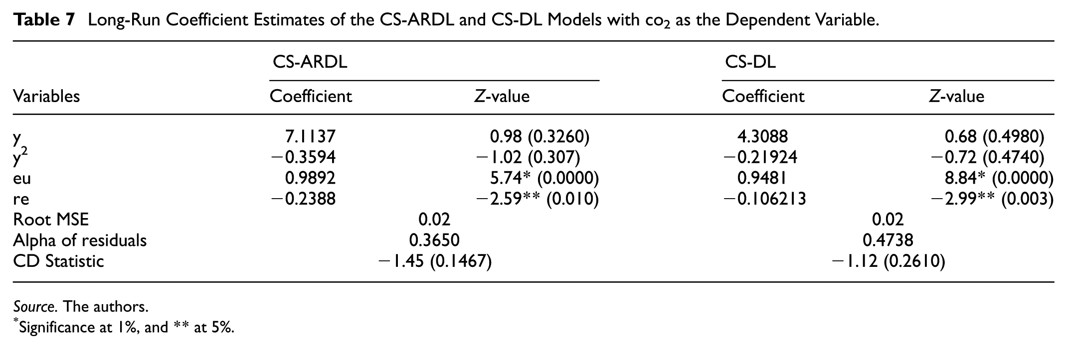
The CS-ARDL regression results are given in Table 7. The adjustment coefficient has a value of −0.93836, which is high and significant. Around 94% of the deviation from the long-run relationship is reduced in a year, suggesting that the long-term relationship is restored quickly. The long-run coefficient of y is 7.11379, while that of y² is −0.35941. None of these figures is significant at 5%. The long-run values of the coefficients, 0.98929 for eu and −0.23882 for re, are statistically significant at the 1% and 5% levels, respectively. The partial adjustment coefficients have a mean group estimate of −0.93836. According to Table 7, this suggests that around 94% of the disequilibrium is corrected annually.

Table 7.

Long-Run Coefficient Estimates of the CS-ARDL and CS-DL Models with co₂ as the Dependent Variable.

	CS-ARDL		CS-DL
Variables	Coefficient	Z-value	Coefficient	Z-value
y	7.1137	0.98 (0.3260)	4.3088	0.68 (0.4980)
y²	−0.3594	−1.02 (0.307)	−0.21924	−0.72 (0.4740)
eu	0.9892	5.74* (0.0000)	0.9481	8.84* (0.0000)
re	−0.2388	−2.59** (0.010)	−0.106213	−2.99** (0.003)
Root MSE	0.02		0.02
Alpha of residuals	0.3650		0.4738
CD Statistic	−1.45 (0.1467)		−1.12 (0.2610)

Source. The authors.

Significance at 1%, and ** at 5%.

The above test statistics do not support an inverted U-shaped curvilinear relationship between y and CO₂. Consequently, the CS-ARDL model results do not support the EKC hypothesis for the OECD countries. Nonetheless, there is evidence to support energy use-driven environmental deterioration and environmental sustainability driven by renewable energy consumption.

CS-DL Approach

CS-DL is a simplification and alternative to CS-ARDL when short-run dynamics are less of a focus. This model directly estimates long-run coefficients using the variables’ distributed lags and their cross-sectional averages. It focuses on the long-run effects directly. It is simpler and more robust in small samples or when the data are highly cross-sectionally dependent. However, the model is less flexible in modelling short-run dynamics than CS-ARDL. The CS-DL estimators exhibit remarkable resilience against misspecifications of dynamics and residual serial correlation. Particularly when T is small, the CS-DL approach’s performance frequently outperforms the alternative panel CS-ARDL estimates (Chudik et al., 2016).

Accounting for cross-sectional dependence, a general ARDL (Py, Px) model including lagged values of the cross-sectional averages of the dependent and independent variables, the corresponding CS-DL model is specified as follows:

\begin{matrix} Y_{i, t} = μ_{i} + θ_{i}^{'} X_{i, t} + \sum_{l = 0}^{p_{x} - 1} δ_{il} Δ X_{i, t - l} + \sum_{l = 0}^{p_{\bar{y}}} ω_{Y, il} {\bar{Y}}_{t - l} \\ + \sum_{l = 0}^{p_{\bar{x}}} ω_{x, il}^{'} {\bar{X}}_{t - l} + e_{it} \end{matrix}

(4)

Where, ${\bar{X}}_{t - l} = N^{- 1} \sum_{i = 1}^{N} X_{it}$ , ${\bar{Y}}_{t} = N^{- 1} \sum_{i = 1}^{N} Y_{it}$ , $p_{\bar{x}}$ is equal to the integer part of $T^{\frac{1}{3}}$ .

Neither y nor y² has a long-term effect on CO₂, as their respective coefficients of 6.94142 and −0.32697 are not significant at either the 1% or 5% level. However, the values of long-run coefficients 0.85398 of eu and −0.1966 of re are significant at the 1% and 5% levels, respectively (Table 7).

We again conclude that there is no inverted U-shaped linkage between CO₂ emissions and GDP per capita since the coefficients of y and y² are not significant. Thus, the CS-DL model’s results also do not provide any evidence to support the EKC hypothesis. However, we find evidence to support both energy use-led environmental degradation and renewable energy consumption-led reduction in emissions, contributing to environmental sustainability.

The results of the CS-DL and CS-ARDL models are robust, as in both cases, the signs of the long-run coefficients of y, y², eu, and re are as expected.

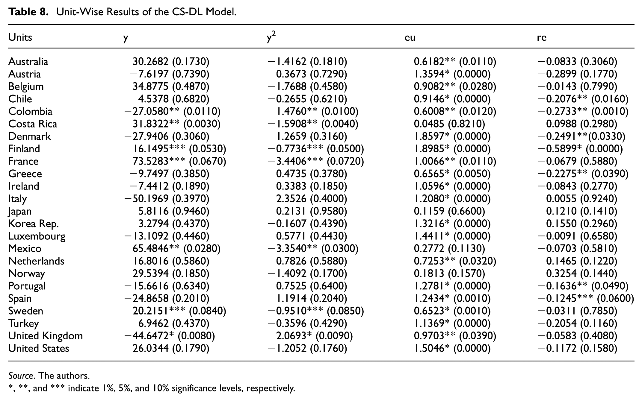
The table below reports the cross-sectional unit-level findings derived from the CS-DL approach. Out of the 24 countries in the sample, only five countries—Costa Rica, Finland, France, Mexico, and Sweden—have results that support the EKC hypothesis. Belgium, Chile, Australia, Austria, Finland, France, Greece, Colombia, Denmark, Ireland, Italy, the Republic of Korea, Spain, Sweden, Turkey, Luxembourg, the Netherlands, Portugal, the United Kingdom, and the United States are among the 20 nations where energy usage is a contributing factor to CO₂ emissions. Increases in the consumption of renewable energy decrease CO₂ emissions in Chile, Colombia, Denmark, Finland, Greece, Portugal, and Spain. Finland is the only country in the sample where both the EKC hypothesis is valid, as well as the growth in the consumption of renewable energy reduces CO₂ emissions (Table 8).

Table 8.

Unit-Wise Results of the CS-DL Model.

Units	y	y²	eu	re
Australia	30.2682 (0.1730)	−1.4162 (0.1810)	0.6182** (0.0110)	−0.0833 (0.3060)
Austria	−7.6197 (0.7390)	0.3673 (0.7290)	1.3594* (0.0000)	−0.2899 (0.1770)
Belgium	34.8775 (0.4870)	−1.7688 (0.4580)	0.9082** (0.0280)	−0.0143 (0.7990)
Chile	4.5378 (0.6820)	−0.2655 (0.6210)	0.9146* (0.0000)	−0.2076** (0.0160)
Colombia	−27.0580** (0.0110)	1.4760** (0.0100)	0.6008** (0.0120)	−0.2733** (0.0010)
Costa Rica	31.8322** (0.0030)	−1.5908** (0.0040)	0.0485 (0.8210)	0.0988 (0.2980)
Denmark	−27.9406 (0.3060)	1.2659 (0.3160)	1.8597* (0.0000)	−0.2491**(0.0330)
Finland	16.1495*** (0.0530)	−0.7736*** (0.0500)	1.8985* (0.0000)	−0.5899* (0.0000)
France	73.5283*** (0.0670)	−3.4406*** (0.0720)	1.0066** (0.0110)	−0.0679 (0.5880)
Greece	−9.7497 (0.3850)	0.4735 (0.3780)	0.6565* (0.0050)	−0.2275** (0.0390)
Ireland	−7.4412 (0.1890)	0.3383 (0.1850)	1.0596* (0.0000)	−0.0843 (0.2770)
Italy	−50.1969 (0.3970)	2.3526 (0.4000)	1.2080* (0.0000)	0.0055 (0.9240)
Japan	5.8116 (0.9460)	−0.2131 (0.9580)	−0.1159 (0.6600)	−0.1210 (0.1410)
Korea Rep.	3.2794 (0.4370)	−0.1607 (0.4390)	1.3216* (0.0000)	0.1550 (0.2960)
Luxembourg	−13.1092 (0.4460)	0.5771 (0.4430)	1.4411* (0.0000)	−0.0091 (0.6580)
Mexico	65.4846** (0.0280)	−3.3540** (0.0300)	0.2772 (0.1130)	−0.0703 (0.5810)
Netherlands	−16.8016 (0.5860)	0.7826 (0.5880)	0.7253** (0.0320)	−0.1465 (0.1220)
Norway	29.5394 (0.1850)	−1.4092 (0.1700)	0.1813 (0.1570)	0.3254 (0.1440)
Portugal	−15.6616 (0.6340)	0.7525 (0.6400)	1.2781* (0.0000)	−0.1636** (0.0490)
Spain	−24.8658 (0.2010)	1.1914 (0.2040)	1.2434* (0.0010)	−0.1245*** (0.0600)
Sweden	20.2151*** (0.0840)	−0.9510*** (0.0850)	0.6523* (0.0010)	−0.0311 (0.7850)
Turkey	6.9462 (0.4370)	−0.3596 (0.4290)	1.1369* (0.0000)	−0.2054 (0.1160)
United Kingdom	−44.6472* (0.0080)	2.0693* (0.0090)	0.9703** (0.0390)	−0.0583 (0.4080)
United States	26.0344 (0.1790)	−1.2052 (0.1760)	1.5046* (0.0000)	−0.1172 (0.1580)

Source. The authors.

, **, and *** indicate 1%, 5%, and 10% significance levels, respectively.

Dumitrescu & Hurlin (D-H) Granger Non-Causality Test

In view of the heterogeneous panels, we used the Granger non-causality test to check for causality from the explanatory variables to the dependent variable following Dumitrescu and Hurlin (2012). A bootstrap process with 700 replications was used to generate the Z-bar values and corresponding p-values. When variables exhibit cross-sectional dependence, the technique of bootstrapping is helpful.

The null hypothesis of the D-H Granger non-causation tests is that there is no Granger causality from one variable to another. The D-H test does not reject the null hypothesis that there is Granger non-causality, either from y to co2 or from co2 to y. The tests also do not reject the null hypothesis of Granger non-causality from y2 to co2 or from co2 to y2. However, the tests reject the Granger non-causality from eu to co2, but do not reject it from co2 to eu. Likewise, the tests do not reject the Granger non-causality from co2 to re, but they reject it from re to co2. Consequently, neither y to co2 nor y² to co2 exhibits Granger causality. Granger causation between eu and co2 and re and co2 is unidirectional (Table 9).

Table 9.

Granger Non-Causality Test of Dumitrescu & Hurlin.

H₀	Z-bar	H₀	Z-bar	Inference
y does not Granger-cause co2	8.9332 (0.1029)	co2 does not Granger-cause y	3.1664 (0.2829)	No Granger causality between y and co2
y² does not Granger-cause co2	8.9422 (0.1029)	co2 does not Granger-cause y²	3.1741 (0.2529)	No Granger-causality between y² and co2
eu does not Granger-cause co2	6.4676*** (0.0757)	co2 does not Granger-cause eu	5.8488 (0.1157)	Granger-causality from eu to co2
re does not Granger-cause co2	15.1838** (0.0029)	co2 does not Granger-cause re	2.1421 (0.4400)	Granger-causality from re to co2

Source. The Authors.

Note.p-Values were computed using 700 bootstrap replications.

Level of significance at 1%, ** at 5%, and *** at 10%.

Surprisingly, our panel data analysis, after adjusting cross-sectional dependence, does not support the EKC theory for the sampled 24 OECD countries, in contrast to the majority of empirical findings (Alam, 2024; Awaworyi Churchill et al., 2018; Ben Jebli et al., 2016; Galeotti et al., 2006; Moomaw & Unruh, 1997) which support the EKC hypothesis based on panel data from OECD countries. For OECD nations, our results accord with (Dijkgraaf & Vollebergh, 2005). It is notable that, like us, cross-sectional dependence was also controlled in (Dijkgraaf & Vollebergh, 2005), whereas other studies have overlooked it. However, this study supports the energy use-led environmental degradation and renewable energy-led environmental sustainability hypotheses, as also supported by previous studies (Alvarez-Herranz et al., 2017; Bilgili et al., 2016; Shafiei & Salim, 2014) for OECD countries.

Energy efficiency and a decrease in CO₂ emissions could result from the transition from non-renewable to renewable energy sources. However, (Jevons, 1866) describes a paradoxical phenomenon in which improvements in energy efficiency may lead to an overall increase in energy consumption rather than a decrease and, therefore, a rise in CO₂ emissions. This paradox can indeed be applied to explain why developed countries may not experience the significant reduction in CO₂ emissions that is expected, despite energy efficiency advances and the integration of renewable energy sources.

Energy efficiency gains may result in lower overall energy expenditures, but they may also raise CO₂ emissions because of increasing energy use. Improved energy efficiency can also lead to economic growth. As economies grow, the demand for energy in various sectors increases, potentially offsetting the benefits of energy efficiency.

CO₂ emissions may also increase due to the Rebound Effect. The rebound effect refers to the phenomenon in which changes in behaviour and consumption patterns partially or wholly offset the expected reductions in energy consumption resulting from efficiency gains. For instance, if vehicles become more fuel-efficient, people might choose to drive more, negating the anticipated reduction in fuel use.

Energy Transition Theory appears to be operating in OECD countries in reducing CO₂ emissions. This theory predicts that the transition from fossil fuel-reliant energy systems to renewable energy systems lowers CO₂ emissions.

To further lessen the rebound effect and ensure that efficiency improvements result in a reduction in energy use and CO₂ emissions, effective laws and incentives are required. Behavioural changes, such as promoting energy conservation and responsible consumption, are crucial.

Therefore, the view that the best way for a country to attain a cleaner environment is through economic growth and development, as argued in (Beckerman, 1992), is not persuasive. Moreover, no empirical study provides evidence and support that economic growth alone enhances environmental quality in a country or region. Hence, relying solely on economic growth is likely to prove futile in the fight against environmental degradation.

For sustainable development, OECD countries should not rely on a high level of income and development. Focussing on optimising energy use and consumption and changing their composition in support of a sustainable environment is the key to combating environmental degradation. The OECD countries need to decrease CO₂ emissions by increasing the share of clean energy in total energy use and decreasing the share of non-renewable energy, especially fossil fuel and biomass, or through the adoption of green or sustainable technology, effective incentive programmes, and prudent environmental regulation in order to achieve sustainable development.

Conclusion and Policy Implications

This study examined the relationship of CO₂ emissions with energy use, renewable energy consumption and tested the EKC theory in OECD countries. We analysed the annual data compiled from the World Bank’s database on World Development Indicators for 24 OECD countries from 1990 to 2016. The five variables included in log form for the analysis are CO₂ emissions per capita, real GDP per capita, the square of real GDP per capita, energy use per capita, and consumption of renewable energy per capita. The test of cross-sectional dependence across cross-sectional units revealed that the panel variables were cross-sectionally dependent. The test of slope heterogeneity indicated that the slopes were heterogeneous across cross-sectional units. In such cases, the appropriate unit root tests for panel variables are the CADF and CIPS tests. Based on these unit root tests, we found the variables to be of mixed order of integration, but none of them was found to be integrated of order more than one. Based on the test of cointegration accounting for cross-sectional dependence, we found the above five variables to be cointegrated.

For a robustness check, we used two methods of the common correlated effects estimator—the CS-DL and CS-ARDL estimators—to estimate the long-term relationship between CO₂ emissions per capita as dependent variable, real GDP per capita, the square of real GDP per capita, energy use per capita, and consumption of renewable energy per capita as the explanatory variables. Reliable and consistent parameter estimates were produced by the CS-ARDL and CS-DL models. The analysis did not find evidence to support the inverted U-shaped relationship between GDP per capita and CO₂ emissions per capita.

Hence, the EKC hypothesis, which postulates an inverse U-shaped relationship between income per capita and CO₂ emissions per capita as a metric of environmental quality, was not supported by the study’s findings. Energy use and CO₂ emissions are positively correlated, but consumption of renewable energy is negatively correlated with CO₂ emissions. Hence, our study did not support the EKC hypothesis for the sampled 24 OECD nations, even after controlling for cross-sectional dependency caused by unobserved common factors. However, this study supports the hypothesis that energy use leads to environmental degradation and that renewable energy consumption promotes environmental sustainability.

Thus, in OECD countries, income growth does not mitigate environmental degradation; energy use causes environmental degradation, but renewable energy consumption promotes environmental quality. The prediction of Energy Transition Theory that the transition from fossil fuel-reliant energy systems to renewable energy systems will lower CO₂ emissions appears to be supported by this study in OECD countries.

Therefore, for a sustainable environment, OECD countries should not rely on economic growth and development. Instead, the key to reducing environmental deterioration is focussing on energy use and renewable energy consumption and altering their composition. OECD countries can directly lower their CO₂ emissions by increasing the use of clean and renewable energy, decreasing the use of non-renewable energy, especially fossil fuels, and leveraging green and sustainable technology. Due to the Jevons’ paradox and rebound effects, energy efficiency gains may also lead to an increase in overall energy consumption. Hence, a comprehensive approach that combines energy efficiency, renewable energy integration, and reductions in overall energy demand is essential for mitigating CO₂ emissions and realising a sustainable environment in OECD countries.

Our study could not control for green technology used across the sampled OECD countries due to the unavailability of data. The non-inclusion of green technology use in OECD countries as an additional control variable may have influenced the results of our study’s estimated model. Hence, a future study may be conducted by including use of green technology as an additional control variable.

Footnotes

Acknowledgements

The authors express their gratitude to Prof. Md. Abdus Salam, Department of Economics, Aligarh Muslim University, for his valuable input to enrich the article.

ORCID iDs

Md. Fakhre Alam

Ajay Singh

Abhishek Tripathi

Reena Singh

Rakesh Kumar

Funding

The authors received no financial support for the research, authorship, and/or publication of this article.

Declaration of Conflicting Interests

The authors declared no potential conflicts of interest with respect to the research, authorship, and/or publication of this article.

Data Availability Statement

The authors declare that all the data used for the article will be made available on request.

References

Ahmed

Khan

A. M.

Bibi

Zakaria

(2017). Convergence of per capita CO₂ emissions across the globe: Insights via wavelet analysis. Renewable and Sustainable Energy Reviews, 75, 86–97. https://doi.org/10.1016/j.rser.2016.10.053

Alam

Fakhre

. (2024). Environmental kuznets curve and sustainable development in OECD countries: A panel data analysis. European Journal of Development Studies, 4(6), 9–15. https://doi.org/10.24018/ejdevelop.2024.4.6.392

Allard

Takman

Uddin

G. S.

Ahmed

(2018). The N-shaped environmental Kuznets curve: an empirical evaluation using a panel quantile regression approach. Environmental Science and Pollution Research, 25(6), 5848–5861. https://doi.org/10.1007/s11356-017-0907-0

Alvarez-Herranz

Balsalobre-Lorente

Shahbaz

Cantos

J. M.

(2017). Energy innovation and renewable energy consumption in the correction of air pollution levels. Energy Policy, 105, 386–397. https://doi.org/10.1016/j.enpol.2017.03.009

Antweiler

Copeland

B. R.

Taylor

M. S.

(2001). Is free trade good for the environment? American Economic Review, 91(4), 877–908. https://doi.org/10.1257/aer.91.4.877

Anwar

Siddique

Sharif

(2021). The moderating role of renewable and non-renewable energy in environment-income nexus for ASEAN countries: Evidence from method of moments quantile regression. Renewable Energy, 164, 956–967. https://doi.org/10.1016/j.renene.2020.09.128

Apergis

(2016). Environmental Kuznets curves: New evidence on both panel and country-level CO₂ emissions. Energy Economics, 54, 263–271. https://doi.org/10.1016/j.eneco.2015.12.007

Apergis

Ozturk

(2015). Testing environmental Kuznets curve hypothesis in Asian countries. Ecological Indicators, 52, 16–22. https://doi.org/10.1016/j.ecolind.2014.11.026

Apergis

Payne

J. E.

Menyah

Wolde-Rufael

(2010). On the causal dynamics between emissions, nuclear energy, renewable energy, and economic growth. Ecological Economics, 69(11), 2255–2260. https://doi.org/10.1016/j.ecolecon.2010.06.014

10.

Arrow

Bolin

Costanza

Dasgupta

Folke

Holling

C. S.

Jansson

B.-O.

Levin

Mäler

K.-G.

Perrings

Pimentel

(1995). Economic growth, carrying capacity, and the environment. Ecological Economics, 15(2), 91–95. https://doi.org/10.1016/0921-8009(95)00059-3

11.

Awaworyi Churchill

Inekwe

Ivanovski

Smyth

. (2018). The Environmental Kuznets curve in the OECD: 1870–2014. Energy Economics, 75, 389–399. https://doi.org/10.1016/j.eneco.2018.09.004

12.

Balsalobre-Lorente

Shahbaz

Roubaud

Farhani

(2018). How economic growth, renewable electricity and natural resources contribute to CO₂ emissions? Energy Policy, 113, 356–367. https://doi.org/10.1016/j.enpol.2017.10.050

13.

Beckerman

(1992). Economic growth and the environment: Whose growth? whose environment? World Development, 20(4), 481–496. https://doi.org/10.1016/0305-750x(92)90038-w

14.

Ben Jebli

Ben Youssef

Ozturk

. (2016). Testing environmental Kuznets curve hypothesis: The role of renewable and non-renewable energy consumption and trade in OECD countries. Ecological Indicators, 60, 824–831. https://doi.org/10.1016/j.ecolind.2015.08.031

15.

Ben Jebli

Farhani

Guesmi

. (2020). Renewable energy, CO₂ emissions and value added: Empirical evidence from countries with different income levels. Structural Change and Economic Dynamics, 53, 402–410. https://doi.org/10.1016/j.strueco.2019.12.009

16.

Bilgili

Koçak

Bulut

. (2016). The dynamic impact of renewable energy consumption on CO 2 emissions: A revisited Environmental Kuznets curve approach. Renewable and Sustainable Energy Reviews, 54, 838–845. https://doi.org/10.1016/j.rser.2015.10.080

17.

Cai

Sam

C. Y.

Chang

(2018). Nexus between clean energy consumption, economic growth and CO₂ emissions. Journal of Cleaner Production, 182, 1001–1011. https://doi.org/10.1016/j.jclepro.2018.02.035

18.

Charfeddine

Kahia

(2019). Impact of renewable energy consumption and financial development on CO₂ emissions and economic growth in the MENA region: A panel vector autoregressive (PVAR) analysis. Renewable Energy, 139, 198–213. https://doi.org/10.1016/j.renene.2019.01.010

19.

Chen

Wang

Zhong

(2019). CO₂ emissions, economic growth, renewable and non-renewable energy production and foreign trade in China. Renewable Energy, 131, 208–216. https://doi.org/10.1016/j.renene.2018.07.047

20.

Chen

Zhao

Lai

Wang

Xia

(2019). Exploring the effects of economic growth, and renewable and non-renewable energy consumption on China’s CO₂ emissions: Evidence from a regional panel analysis. Renewable Energy, 140, 341–353. https://doi.org/10.1016/j.renene.2019.03.058

21.

Chudik

Mohaddes

Pesaran

M. H.

Raissi

(2016). Long-run effects in large heterogeneous panel data models with cross-sectionally correlated errors (pp. 85–135). Emerald Group. https://doi.org/10.1108/S0731-905320160000036013

22.

Chudik

Pesaran

M. H.

(2015). Common correlated effects estimation of heterogeneous dynamic panel data models with weakly exogenous regressors. Journal of Econometrics, 188(2), 393–420. https://doi.org/10.1016/j.jeconom.2015.03.007

23.

Dahmani

Mabrouki

Ben Youssef

(2023). The ICT, financial development, energy consumption and economic growth nexus in MENA countries: dynamic panel CS-ARDL evidence. Applied Economics, 55(10), 1114–1128. https://doi.org/10.1080/00036846.2022.2096861

24.

Demissew Beyene

Kotosz

. (2020). Testing the environmental Kuznets curve hypothesis: An empirical study for East African countries. International Journal of Environmental Studies, 77(4), 636–654. https://doi.org/10.1080/00207233.2019.1695445

25.

Dijkgraaf

Vollebergh

H. R. J.

(2005). A test for parameter homogeneity in CO₂ panel EKC estimations. Environmental & Resource Economics, 32(2), 229–239. https://doi.org/10.1007/s10640-005-2776-0

26.

Ditzen

(2021). Estimating long-run effects and the exponent of cross-sectional dependence: An update to xtdcce2. The Stata Journal: Promoting Communications on Statistics and Stata, 21(3), 687–707. https://doi.org/10.1177/1536867X211045560

27.

Dogan

Seker

(2016). Determinants of CO₂ emissions in the European Union: The role of renewable and non-renewable energy. Renewable Energy, 94, 429–439. https://doi.org/10.1016/j.renene.2016.03.078

28.

Dong

Hochman

Zhang

Sun

Liao

(2018). CO₂ emissions, economic and population growth, and renewable energy: Empirical evidence across regions. Energy Economics, 75, 180–192. https://doi.org/10.1016/j.eneco.2018.08.017

29.

Dong

Sun

Jiang

Zeng

(2018). CO₂ emissions, economic growth, and the environmental Kuznets curve in China: What roles can nuclear energy and renewable energy play? Journal of Cleaner Production, 196, 51–63. https://doi.org/10.1016/j.jclepro.2018.05.271

30.

Dumitrescu

E.-I.

Hurlin

(2012). Testing for Granger non-causality in heterogeneous panels. Economic Modelling, 29(4), 1450–1460. https://doi.org/10.1016/j.econmod.2012.02.014

31.

Everaert

De Groote

(2016). Common correlated effects estimation of dynamic panels with cross-sectional dependence. Econometric Reviews, 35(3), 428–463. https://doi.org/10.1080/07474938.2014.966635

32.

Galeotti

Lanza

Pauli

(2006). Reassessing the environmental Kuznets curve for CO₂ emissions: A robustness exercise. Ecological Economics, 57(1), 152–163. https://doi.org/10.1016/j.ecolecon.2005.03.031

33.

Grossman

G. M.

Krueger

A. B.

(1991). Environmental impacts of a North American free trade agreement. NBER. https://doi.org/10.3386/w3914

34.

Grossman

G. M.

Krueger

A. B.

(1995). Economic growth and the environment. The Quarterly Journal of Economics, 110(2), 353–377. https://doi.org/10.2307/2118443

35.

Heerink

Mulatu

Bulte

(2001). Income inequality and the environment: aggregation bias in environmental Kuznets curves. Ecological Economics, 38(3), 359–367. https://doi.org/10.1016/S0921-8009(01)00171-9

36.

Heil

M. T.

Selden

T. M.

(2001). International Trade Intensity and Carbon Emissions: A Cross-Country Econometric Analysis. The Journal of Environment & Development, 10(1), 35–49. https://doi.org/10.1177/107049650101000103

37.

Hosier

R. H.

Dowd

(1987). Household fuel choice in Zimbabwe. Resources and Energy, 9(4), 347–361. https://doi.org/10.1016/0165-0572(87)90003-X

38.

Inglesi-Lotz

Dogan

(2018). The role of renewable versus non-renewable energy to the level of CO₂ emissions a panel analysis of sub- Saharan Africa’s βig 10 electricity generators. Renewable Energy, 123, 36–43. https://doi.org/10.1016/j.renene.2018.02.041

39.

Işık

Ongan

Özdemir

(2019). Testing the EKC hypothesis for ten US states: an application of heterogeneous panel estimation method. Environmental Science and Pollution Research, 26(11), 10846–10853. https://doi.org/10.1007/s11356-019-04514-6

40.

Jevons

W. S.

(1866). The coal question: An Inquiry concerning the progress of the nation, and the probable exhaustion of our coal mines (Second). Macmillan and Co.

41.

Kaufmann

R. K.

Davidsdottir

Garnham

Pauly

(1998). The determinants of atmospheric SO2 concentrations: reconsidering the environmental Kuznets curve. Ecological Economics, 25(2), 209–220. https://doi.org/10.1016/S0921-8009(97)00181-X

42.

Khan

M. A.

Ozturk

(2020). Examining foreign direct investment and environmental pollution linkage in Asia. Environmental Science and Pollution Research, 27(7), 7244–7255. https://doi.org/10.1007/s11356-019-07387-x

43.

Kuznets

(1955). Economic growth and income inequality. American Economic Review, 45(1), 1–30.

44.

Lau

L.-S.

Choong

C.-K.

C.-F.

Liew

F.-M.

Ching

S.-L.

(2019). Is nuclear energy clean? Revisit of Environmental Kuznets curve hypothesis in OECD countries. Economic Modelling, 77, 12–20. https://doi.org/10.1016/j.econmod.2018.09.015

45.

Lekakis

J. N.

Kousis

(2001). Demand for and supply of environmental quality in the environmental Kuznets curve hypothesis. Applied Economics Letters, 8(3), 169–172. https://doi.org/10.1080/13504850150504531

46.

Liu

Zhang

Bae

(2017). The impact of renewable energy and agriculture on carbon dioxide emissions: Investigating the environmental Kuznets curve in four selected ASEAN countries. Journal of Cleaner Production, 164, 1239–1247. https://doi.org/10.1016/j.jclepro.2017.07.086

47.

Magnani

(2000). The environmental Kuznets curve, environmental protection policy and income distribution. Ecological Economics, 32(3), 431–443. https://doi.org/10.1016/S0921-8009(99)00115-9

48.

Ahmad

Oei

P.-Y.

(2021). Environmental Kuznets curve in France and Germany: Role of renewable and nonrenewable energy. Renewable Energy, 172, 88–99. https://doi.org/10.1016/j.renene.2021.03.014

49.

McConnell

K. E.

(1997). Income and the demand for environmental quality. Environment and Development Economics, 2(4), 383–399. https://doi.org/10.1017/S1355770X9700020X

50.

Menyah

Wolde-Rufael

(2010). CO₂ emissions, nuclear energy, renewable energy and economic growth in the US. Energy Policy, 38(6), 2911–2915. https://doi.org/10.1016/j.enpol.2010.01.024

51.

Mikayilov

J. I.

Galeotti

Hasanov

F. J.

(2018). The impact of economic growth on CO₂ emissions in Azerbaijan. Journal of Cleaner Production, 197, 1558–1572. https://doi.org/10.1016/j.jclepro.2018.06.269

52.

Mirza

F. M.

Kanwal

(2017). Energy consumption, carbon emissions and economic growth in Pakistan: Dynamic causality analysis. Renewable and Sustainable Energy Reviews, 72, 1233–1240. https://doi.org/10.1016/j.rser.2016.10.081

53.

Moomaw

W. R.

Unruh

G. C.

(1997). Are environmental Kuznets curves misleading us? The case of CO₂ emissions. Environment and Development Economics, 2(4), 451–463. https://doi.org/10.1017/s1355770x97000247

54.

Namahoro

J. P.

Nzabanita

(2021). The impact of total and renewable energy consumption on economic growth in lower and middle- and upper-middle-income groups: Evidence from CS-DL and CCEMG analysis. Energy, 237, 121536. https://doi.org/10.1016/j.energy.2021.121536

55.

OECD. (2023). Environment at a Glance Indicators. OECD Publishing, Paris. https://doi.org/10.1787/ac4b8b89-en

56.

Okumus

Guzel

A. E.

Destek

M. A.

(2021). Renewable, non-renewable energy consumption and economic growth nexus in G7: Fresh evidence from CS-ARDL. Environmental Science and Pollution Research, 28(40), 56595–56605. https://doi.org/10.1007/s11356-021-14618-7

57.

Panayotou

(1993). Empirical tests and policy analysis of environmental degradation at different stages of economic development (wp 238). World Employment Programme Research Working Paper. Technology and Employment Programme). https://webapps.ilo.org/public/libdoc/ilo/1993/93B09_31_engl.pdf

58.

Pesaran

M. H.

(2006). Estimation and inference in large heterogeneous panels with a multifactor error structure. Econometrica, 74(4), 967–1012. https://doi.org/10.1111/j.1468-0262.2006.00692.x

59.

Pesaran

M. H.

(2007). A simple panel unit root test in the presence of cross-section dependence. Journal of Applied Economics, 22(2), 265–312. https://doi.org/10.1002/jae.951

60.

Pesaran

M. H.

(2015). Testing weak cross-sectional dependence in large panels. Econometric Reviews, 34(6-10), 1089–1117. https://doi.org/10.1080/07474938.2014.956623

61.

Petinrin

J. O.

Shaaban

(2015). Renewable energy for continuous energy sustainability in Malaysia. Renewable and Sustainable Energy Reviews, 50, 967–981. https://doi.org/10.1016/j.rser.2015.04.146

62.

Porter

M. E.

Linde

C. V. D.

(1995). Toward a new conception of the environment-competitiveness relationship. Journal of Economic Perspectives, 9(4), 97–118. https://doi.org/10.1257/jep.9.4.97

63.

Quek

Wah

T. Y.

(2018). Challenges in environmental sustainability of renewable energy options in Singapore. Energy Policy, 122, 388–394. https://doi.org/10.1016/j.enpol.2018.07.055

64.

Rana

Ingrao

Lombardi

Tricase

(2016). Greenhouse gas emissions of an agro-biogas energy system: Estimation under the renewable energy directive. Science of the Total Environment, 550, 1182–1195. https://doi.org/10.1016/j.scitotenv.2015.10.164

65.

Roca

(2003). Do individual preferences explain the Environmental Kuznets curve? Ecological Economics, 45(1), 3–10. https://doi.org/10.1016/s0921-8009(02)00263-x

66.

Shafiei

Salim

R. A.

(2014). Non-renewable and renewable energy consumption and CO₂ emissions in OECD countries: A comparative analysis. Energy Policy, 66, 547–556. https://doi.org/10.1016/j.enpol.2013.10.064

67.

Shafik

Bandyopadhya

(1992). Economic growth and environmental quality. Policy, research working papers; no. WPS 904. World development report Washington, D.C.: World Bank Group. http://documents.worldbank.org/curated/en/833431468739515725

68.

Sharif

Raza

S. A.

Ozturk

Afshan

(2019). The dynamic relationship of renewable and nonrenewable energy consumption with carbon emission: A global study with the application of heterogeneous panel estimations. Renewable Energy, 133, 685–691. https://doi.org/10.1016/j.renene.2018.10.052

69.

Shi

(2003). The impact of population pressure on global carbon dioxide emissions, 1975–1996: Evidence from pooled cross-country data. Ecological Economics, 44(1), 29–42. https://doi.org/10.1016/S0921-8009(02)00223-9

70.

Sinha

Shahbaz

(2018). Estimation of environmental Kuznets curve for CO₂ emission: Role of renewable energy generation in India. Renewable Energy, 119, 703–711. https://doi.org/10.1016/j.renene.2017.12.058

71.

Smil

(2016). Energy Transitions. ABC-CLIO, LLC. https://doi.org/10.5040/9798400646126

72.

Sohail

Abbasi

B. N.

(2023). Exploring the interrelationship among health status, CO₂ emissions, and energy use in the top 20 highest emitting economies: based on the CS-DL and CS-ARDL approaches. Air Quality Atmosphere & Health, 16(7), 1–24. https://doi.org/10.1007/s11869-023-01350-z

73.

Sorrell

(2007). The Rebound effect: an assessment of the evidence for economy-wide energy savings from improved energy efficiency. UK Energy Research Centre (UKERC).

74.

Stern

D. I.

(1998). Progress on the environmental Kuznets curve? Environment and Development Economics, 3(2), 173–196. https://doi.org/10.1017/s1355770x98000102

75.

Stern

D. I.

(2004). The Rise and fall of the Environmental Kuznets curve. World Development, 32(8), 1419–1439. https://doi.org/10.1016/j.worlddev.2004.03.004

76.

Ulucak

Bilgili

(2018). A reinvestigation of EKC model by ecological footprint measurement for high, middle and low income countries. Journal of Cleaner Production, 188, 144–157. https://doi.org/10.1016/j.jclepro.2018.03.191

77.

Unruh

G. C.

(2000). Understanding carbon lock-in. Energy Policy, 28(12), 817–830. https://doi.org/10.1016/S0301-4215(00)00070-7

78.

D. H.

A. T.

C. M.

Nguyen

H. M.

(2020). The role of renewable energy, alternative and nuclear energy in mitigating carbon emissions in the CPTPP countries. Renewable Energy, 161, 278–292. https://doi.org/10.1016/j.renene.2020.07.093

79.

Wang

Fang

(2018). Urbanization, economic growth, energy consumption, and CO₂ emissions: Empirical evidence from countries with different income levels. Renewable and Sustainable Energy Reviews, 81, 2144–2159. https://doi.org/10.1016/j.rser.2017.06.025

80.

Westerlund

(2007). Testing for error correction in panel data. Oxford Bulletin of Economics and Statistics, 69(6), 709–748. https://doi.org/10.1111/j.1468-0084.2007.00477.x

81.

Yang

Abbas

Hanif

Alharthi

Taghizadeh-Hesary

Aziz

Mohsin

(2021). Short- and long-run influence of energy utilization and economic growth on carbon discharge in emerging SREB economies. Renewable Energy, 165, 43–51. https://doi.org/10.1016/j.renene.2020.10.141

82.

Yao

Zhang

(2019). Renewable energy, carbon emission and economic growth: A revised environmental Kuznets curve perspective. Journal of Cleaner Production, 235, 1338–1352. https://doi.org/10.1016/j.jclepro.2019.07.069

83.

Zhang

Liu

(2019). The roles of international tourism and renewable energy in environment: New evidence from Asian countries. Renewable Energy, 139, 385–394. https://doi.org/10.1016/j.renene.2019.02.046

84.

Zoundi

(2017). CO₂ emissions, renewable energy and the environmental Kuznets curve, a panel cointegration approach. Renewable and Sustainable Energy Reviews, 72, 1067–1075. https://doi.org/10.1016/j.rser.2016.10.018

Linkages Among Income,Renewable Energy Consumption and CO 2 Emissions and their Implications for Sustainable Development in the OECD Countries

Abstract

Plain language summary

Keywords

Introduction

Theoretical Underpinnings

The EKC Theory

Energy Ladder Theory

Decoupling Theory

Energy Transition Theory

Carbon Lock-In Theory

Porter’s Hypothesis

Rebound Effect Theory

Structural Change Theory

Literature Review

Data and Model Specification

Results and Discussion

Cross-Sectional Dependence Test

Slope Heterogeneity Test

Panel Unit Root Tests

Test of Cointegration

CS-ARDL and CS-DL Models

CS-ARDL Approach

CS-DL Approach

Dumitrescu & Hurlin (D-H) Granger Non-Causality Test

Conclusion and Policy Implications

Footnotes

Acknowledgements

ORCID iDs

Funding

Declaration of Conflicting Interests

Data Availability Statement

References