Sage Journals: Discover world-class research

Abstract

Coase assumed that firms only use balance-sheet financing for their capital investments. Other forms of financing exist, and as shown, the process by which economic utility theory gets applied to Internalization Theory is found to be contingent on the method of financing. Coase’s underlying financing assumption causes the long-standing Investment Opportunity Schedule (IOS) to yield erroneous results when applied to project-financed investments. This is significant because project financing is now a $200+ billion annual global market and widely used to finance electric power projects and numerous other capital-intensive investments. A new investment ranking mechanism (the MIOS) is proposed and shown to be the proper ranking mechanism for project-financed investment opportunities. Support is found for the new investment ranking mechanism using a paired comparison methodology which yields the ranking of the potential investments to be internalized as well as the placement of the equilibrium point. As shown, the Coasian IOS is not universal, but rather, is contingent on the method of financing. Thus, the answers to Coase’s two seminal questions which form the basis for Internalization Theory (Which business opportunities should be internalized by a firm?, and What should be the extent or boundary of a firm?) are also shown to be contingent on the method of financing. The IOS and the MIOS, working in tandem, provide a better foundation for Internalization Theory.

JEL Codes: D21, D23, G31.

Plain Language Summary

The Need to Fix the Investment Opportunity Schedule Due to Coase’s “Hidden in Plain Sight” Assumption

The Investment Opportunity Schedule (IOS) has been universally taught to finance students for almost 100 years to demonstrate which investments should be rationally accepted or rejected. However, this paper uncovers a hidden assumption in the IOS which restricts its applicability to balance-sheet financing. Other types of financing have become common, such as project-financing which has grown into a $200+ billion/yr global market. This creates a problem because the IOS forms the foundation of Internalization Theory and a significant portion of International Business studies are based on Internalization Theory. A new methodology is developed, the Modified IOS (MIOS), which is shown to be correct for evaluating project-financing investments by making use of a quantitative analysis method, Paired Comparison Best Worst Scaling, which has been used previously in willingness-to-pay economic analyses. Financial analysts should replace the IOS with the MIOS for project-financed investments. The IOS and the MIOS, working in tandem, provide a more solid foundation for Internalization Theory.

Keywords

Coasian Investment opportunity schedule internalization theory paired comparison methodology project financing

Introduction

In The Nature of the Firm, Coase (1937) addressed why firms exist, and in the process, presented and answered two important questions: 1) Which business opportunities should a firm choose to internalize, and 2) What should be the extent or boundary of a firm? In this seminal work, Coase put forth his marginal cost/marginal benefit logic leading to the conclusion that a business should choose to expand (i.e., to internalize or bring business activities inside the firm) up to the point at which it costs the firm the same to “make or buy.” This logic provides the foundation for Internalization Theory (Buckley, 1988; Rugman, 1986; Verbeke, 2005) which, when distilled down to its essence, states that a firm maximizes its value by bringing inside the firm only those activities that possess positive economic utility (the marginal benefits of organizing the activity internally exceed the marginal costs). Other activities (those with negative utility) should remain external to the firm and the output of those activities procured by the firm in the open market. As Coase expressed, “A firm expands to the point where an additional allocative measure costs more internally than it would through a contract on markets” (Coase, 1937, p. 395).

Coase assumed, without any mention and thus “hidden in plain sight” until now, that firms only use balance-sheet financing for their capital investments (see Section II.2 regarding Coase’s treatment of the firm’s weighted average cost of capital as evidence of his balance-sheet financing assumption). However, today, other forms of financing exist and comprise a significant portion of the financing market (Baldauf & Jochem, 2024; Clifford, 2020; Fight, 2006; Yescombe, 2002).

As shown herein, the process by which economic utility theory gets applied to Internalization Theory is found to be contingent on the method of financing, and as a result, the answers to Coase’s two seminal questions which form the foundation for Internalization Theory are also found to be contingent on the method of financing. Coase’s assumption of balance-sheet financing can cause the long-standing Investment Opportunity Schedule (IOS) to yield erroneous results when applied to project-financed investments, and thus, is unable to provide a foundation for Internalization Theory research studies that include any project-financed investments. This is significant because project financing is now a $200+ billion annual global market and is widely used to finance electric power projects and numerous other capital-intensive investments. It is, therefore, time to rethink Internalization Theory, and in doing so, this paper contributes new insights that contribute to the economics of Internalization Theory. In particular:

1) This paper unearths a theoretical assumption in Coase (1937) not previously addressed in the literature that limits the applicability of the IOS to balance-sheet financing, raises a fundamental question about Internalization Theory, and sheds new light on how economic utility theory is to be applied to Internalization Theory;

2) This paper sets forth a new investment ranking mechanism, consistent with the marginal cost/marginal benefit logic used by Coase, called the Modified Investment Opportunity Schedule (MIOS) which is shown to be the proper ranking mechanism for project-financed investment opportunities, and which fills a long-overlooked gap in Internalization Theory literature; and

3) This paper performs a quantitative experimental design analysis that provides statistical support for the new investment ranking mechanism using a paired comparison methodology having significant precedent in economics and finance literature involving willingness-to-pay analyses (Kingsley & Brown, 2013; Louviere & Islam, 2008; Rausch et al., 2021; Samarzija, 2019; Tanaka et al., 2022; USDA, 2023).

The main purpose of this paper is not to add to the plethora of existing investment evaluation methods. Rather, its purpose is to focus on the development and use of the IOS which forms the foundation for Internalization Theory. Specifically:

1) The traditional IOS is shown to be limited to balance-sheet financing due to this paper’s uncovering of a hidden assumption;

2) As a result, Internalization Theory has been resting improperly on the traditional IOS for its foundational support;

3) To correct this, a new method is developed, the Modified IOS (MIOS); and

4) The IOS and MIOS, working in tandem, provide a proper foundation for Internalization Theory.

Conceptual Development

Internalization Theory

Coase set forth in great detail the importance of understanding the relationship between a firm’s efficiency and size, and from this, an understanding of which potential activities should be organized within the firm and which should remain external (Coase, 1937). The organizing of these opportunities by rank order has become known as the investment opportunity schedule (IOS) with the Coasian equilibrium point occurring where marginal benefits equal marginal costs (Brigham, 1979; Kay, 2015; Williamson, 1975). Stated another way, the equilibrium point is where the internal rate of return (IRR) of each of the various investment opportunities, ranked from highest to lowest, intersects the firm’s weighted average cost of capital (WACC). Thus, all investment opportunities that have an IRR greater than the firm’s WACC should be selected by management to be internalized (i.e., brought in-house or inside) by the firm, and this then defines the boundary or the extent of the firm (Brigham, 1979; Coase, 1937; Kay, 2015; Williamson, 1975). See Figure 1, familiar to practitioners of economics and finance, which depicts the equilibrium. It would be economically irrational for a firm to extend beyond this point by investing in a project having an IRR that is less than the firm’s WACC (Brigham, 1979; Coase, 1937; Kay, 2015; Williamson, 1975).

Figure 1.

The investment opportunity schedule.

Coase’s ranking of investment opportunities rests on marginal utility theory which extends back in time for centuries, and per Kay (2015), Coase viewed the organizing of transactions in terms of marginal analyses. As shown in Figure 1, the firm should invest in projects A, B, and C because they provide an increase in utility to the firm, that is, their marginal benefits exceed their marginal costs or IRR > WACC. The firm should not invest in projects D and E because they do not provide positive marginal utility, that is, their marginal benefits do not exceed their marginal costs.

This choice to invest or not invest in a project (i.e., whether to bring production costs internal to a firm or keep them external) forms the foundation of Internalization Theory (Buckley, 1988). Rugman (1986), the economic choice of action is to be based on the costs and benefits of the activities being evaluated. Firms grow by internalizing investment opportunities until they are no longer cost-effective (Buckley, 1988). Internalization can be a two-way street; markets are not static but dynamic causing a re-evaluation of equilibrium which may lead to further investment or the divestment of past investment, as the case may be, to maximize the efficiency of the firm (Buckley, 1988; Coase, 1937; Rugman, 1986). Rugman (1986) and Verbeke (2005) have shown that internalization is a rational response to imperfect markets (thereby increasing the efficiency of the firm), and a firm’s internalization of a market inefficiency can increase the efficiency of the market. More recently, Buckley and Casson (2009) affirmed that Coase’s work provided the underlying theory of internalization. In summation, for the past 40 years, many researchers have labeled Internalization Theory as central to the study of proper business management (Brigham & Ehrhardt, 2017; Buckley, 1988; Buckley & Casson, 2009; Caves, 1996; Hennart, 1988; Narula et al., 2019; Ross et al., 2016; Rugman, 1986; Verbeke, 2005) and the IOS has withstood the test of time when applied to balance sheet financing.

The Change from Balance Sheet to Project Financing

Yet, during the same 40 years, the use of balance sheet financing has often been replaced by project financing in various markets including real estate, oil and gas drilling, and electricity generation (Baldauf & Jochem, 2024; Clifford, 2020; Fight, 2006; Klompjan & Wouters, 2002; Yescombe, 2002). For example, every electric power project within deregulated electricity markets uses project financing (Buscaino et al., 2012; Jadidi et al., 2020; Kaminker, 2017; Mora et al., 2019). Its use is international and has grown into a $200+ billion per year financing market (Fight, 2006; Yescombe, 2002). This changeover was largely driven by two advantages: project financing helps to manage risk by preventing recourse to an affiliate (including the parent company) in the event of a project’s default and it also makes repossession of an asset by the lender following a default less encumbered (Baldauf & Jochem, 2024; Clifford, 2020; Fight, 2006; Klompjan & Wouters, 2002; Yescombe, 2002).

Coase assumed without providing any discussion that the WACC curve shown in Figure 1 always had a slope greater than zero (Coase, 1937). He also assumed the WACC assigned to each potential investment is dependent on the WACC of those projects that “line up” in the IOS ahead of the investment (since the slope of the WACC curve was greater than zero). These are proper assumptions for firms that use balance-sheet financing for their capital investments (Baumol & Malkiel, 1967; Brigham, 1979; Ross et al., 2016), but these restrictions do not apply for project-financing where the WACC for a project-financed investment is independent of the other project-financed investments under consideration and, as discussed further in the next section, the WACC for a project-financed investment is independent of the parent’s WACC. When project financing is used, the two assumptions made by Coase noted above no longer apply, which permits the slope of the WACC curve in Figure 1 to turn negative. Because Coase applied the above restrictions in his treatment of the WACC, it is now evident that he assumed balance-sheet financing and no other forms of financing.

Coase’s balance-sheet financing assumption and its lack of discussion were not unreasonable since project financing was little known when his paper was published. However, since the 1980s, the use of project financing spread globally and has become commonplace (Baldauf & Jochem, 2024; Clifford, 2020; Yescombe, 2002). A review of the literature yields numerous published papers that discuss the IOS and Coase’s foundational contribution to Internalization Theory, but none that discuss Coase’s financing assumption, or that examine the critical difference between the alternate assumptions of balance sheet and project financing and its effect on the IOS and Internalization Theory. Until now, Coase’s financing assumption and its implication remained overlooked. How ironic that Coase’s opening words in his seminal work were:

Economists in building up a theory have often omitted to examine the foundations on which it was erected. This examination is, however, essential not only to prevent the misunderstanding and needless controversy which arise from a lack of knowledge of the assumptions on which a theory is based, but also because of the extreme importance for economics of good judgment in choosing between rival sets of assumptions (Coase, 1937, p. 386).

Such is the case here. There is a rival set of assumptions (i.e., balance sheet financing versus project financing) and a review of the literature suggests that economists during the past 40 years have omitted one of them in the building up of Internalization Theory from its foundations. Yet, every day during the past 40 years, firms have internalized balance-sheet financed and project-financed investments. A review also finds that the literature is devoid of an investment ranking mechanism like the IOS that is applicable for project-financed investments. This paper fills these gaps by 1) identifying the importance of the distinctly different underlying assumptions, 2) shedding new light on how economic utility theory is to be applied to Internalization Theory, 3) offering a new ranking system for firms that use project-financing, and 4) providing a broader foundational support for Internalization Theory.

Identification of the Problem

The lack of an investment ranking mechanism applicable to project-financed investments is problematic because, as shown in section “The View From the Perspective of the Investing Company,” the Coasian IOS yields erroneous results when used to determine which project-financed investment opportunities should be internalized. In turn, this creates problems when used to determine the extent or boundary of a firm that makes use of project-finance. With project-finance, it is the WACC of the project that is relevant, and not the WACC of the firm as used in the Coasian IOS. Project financing is a separable capital investment owned by a special purpose company in which the lenders look to the cash flow of the project to service their loans (Baldauf & Jochem, 2024; Buscaino et al., 2012; Clifford, 2020; Fight, 2006; Klompjan & Wouters, 2002; Ugboma, 2021; Yescombe, 2002). Unlike balance-sheet financing, project financing provides an impenetrable, non-recourse “wall” between the project and the balance sheet of the investing firm that prevents the lender from accessing the cash of the parent company and from relying on the parent company’s balance sheet (Baldauf & Jochem, 2024; Clifford, 2020; Fight, 2006; Klompjan & Wouters, 2002; Ugboma, 2021; Yescombe, 2002). The investing firm’s WACC is immaterial as both the project’s cost of debt and its debt to equity (D:E) ratio are different from that of the investing firm. In addition, when the project is a joint venture, the project’s cost of equity is a function of all the venture’s investing partners. Thus, the WACC of a project-financed project bears little relation to the WACC of the investing company, and this is what leads the Coasian IOS to yield erroneous results when applied to project financing.

This can be elementarily exemplified as follows: Assume a 50:50 joint venture that will be project-financed on a non-recourse basis with an 80:20 D:E ratio. The equity invested into the JV comes from the two parent companies and the cost of this equity would be the WACC of each of the parent companies. The debt for the JV would be provided by one or more lenders, typically acting together in a consortium so that there is only one debt instrument. This gives us:

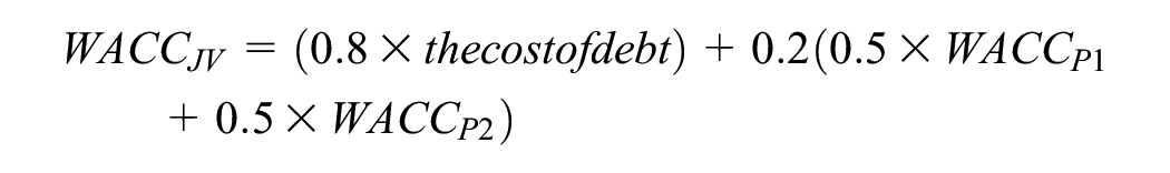
W A C C_{J V} = (0.8 \times t h e c o s t o f d e b t) + 0.2 (0.5 \times W A C C_{P 1} + 0.5 \times W A C C_{P 2})

where

WACC_JV is the weighted average cost of capital of the project-financed joint venture project,

WACC_P1 is the equity investment into the joint venture project from parent company#1, and

WACC_P2 is the equity investment into the joint venture project from parent company#2.

Clearly, WACC_JV doesn’t equal WACC_P1 or WACC_P2, and this is why the Coasian IOS yields erroneous results when applied to project financing. Similarly, it yields erroneous results when answering Coase’s two seminal questions: 1) Which business opportunities should be internalized by a firm, and 2) What is the extent or boundary of a firm?

The Modified IOS

To address this problem, this paper introduces a new investment ranking mechanism that is designed for ranking and internalizing project-financed investments: the Modified IOS. Like the Coasian IOS, its roots are in marginal utility theory, and like the Coasian IOS, it is based on a comparison of marginal costs and marginal benefits. The Modified IOS (MIOS) differs from the traditional IOS in that it considers each project’s specific WACC rather than the WACC of the investing company.

The Modified IOS ranks, from highest to lowest, the project-financed investment opportunities available to a firm based upon a ratio of their IRR to WACC. Thus, where the Coasian IOS first ranks the investment opportunities based solely on their respective IRR and then compares this ranking against the firm’s WACC (as shown in Figure 1), this new MIOS first calculates the IRR to WACC ratio for each project (an indication of each project’s expected utility) and then ranks their ratios. Under the Coasian IOS, the source of funding (debt and equity) for each investment opportunity comes through and from a single source – the parent company. The MIOS, in contrast, recognizes that the funding (debt and equity) for each project-financed investment opportunity comes through and from multiple sources (equity from the parent company(s) and debt from the project finance lenders). In a sense, each project is its own firm with its own WACC, and the investor is rank-ordering the expected utility of the different firms. (N.B. This analogy borrows from, but is different from, the well-studied case of a firm using its WACC to invest in a portfolio of companies.) Thus, while the Coasian IOS remains an effective tool to rank investment opportunities that are financed based on the balance sheet of a company (Brigham & Ehrhardt, 2017; Ross et al., 2016), the MIOS appears to be the proper ranking of project-financed investment opportunities because it takes into account the individual project’s own WACC prior to rank-ordering so that the ranking is based on the projects’ expected utility, not their IRR as per Coase. Doing so yields a correct ranking for project-financed investments, even when viewed from the perspective of the investing company.

The View from the Perspective of the Investing Company

To illustrate the view from the perspective of the investing company, assume a parent company that owns electric power projects in a deregulated market. As is typical for this context, all of the company’s projects make use of project financing that is non-recourse to the parent company. At this time, the company has four potential power plant investment opportunities. The IRR and WACC for each of the four opportunities are presented in Table 1 along with a calculation of their IRR:WACC ratios.

Table 1.

MIOS Ranking Example.

Project	IRR	WACC	IRR:WACC	MIOS Rank
A	20	25	0.8	4
B	15	12	1.25	2
C	15	15	1.0	3
D	10	5	2.0	1

Source: Authors’ own work.

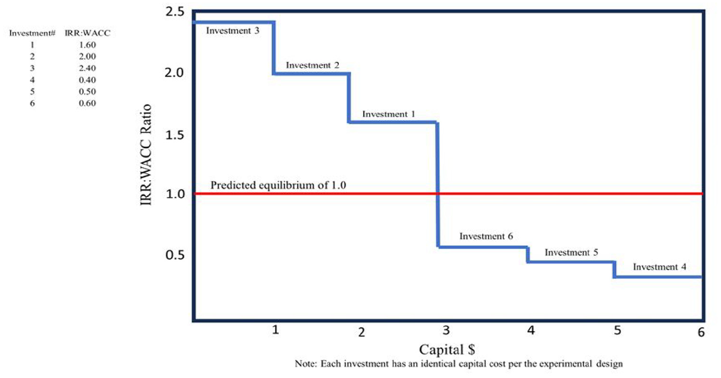
Project A has the highest IRR and would have therefore been ranked first on the Coasian IOS, but project A provides the least expected utility (actually, negative) and is thus ranked last by the MIOS. Project D with an IRR of 10% would be ranked last on the Coasian IOS but is ranked first here because it provides the highest expected utility. Projects A and D thereby illustrate why the Coasian IOS cannot be used for project-financed projects. Both the Coasian IOS and the MIOS arrive at the same conclusion that the parent company should be indifferent about investing in project C which has an IRR:WACC ratio of unity. See Figure 2 which depicts the four projects. Note that the vertical axis in Figure 2 differs from that in Figure 1 as “percent” has been replaced by “IRR:WACC ratio.”

Figure 2.

The modified investment opportunity schedule.

Projects D, B, and C (in that order) have an IRR:WACC ratio equal to or higher than 1.0 and thus should be internalized by the company, while project A should be kept external as its IRR:WACC ratio is less than unity. Project C sets the extent or boundary of the firm as its IRR:WACC ratio is unity. This leads to the following two hypotheses which parallel the two questions posed by Coase:

H1: When making use of project financing, as opposed to balance sheet financing, the boundary or extent of the firm is established at an IRR:WACC ratio of unity.

H2: When making use of project financing, as opposed to balance sheet financing, those investment opportunities for which the IRR:WACC ratio is greater than or equal to unity should be internalized by the firm.

Methodology

If the proposed theoretical construct is correct (i.e., that the MIOS appears to be a more appropriate ranking mechanism for project-financed investment opportunities), then it should be possible to observe behavior that aligns with this theoretical construct. Private data from multiple companies is not expected to be reasonably available. On the other hand, it is possible to design an experiment that replicates the decision-making environment, enables the quantification of this behavior, and generates sufficient data for quantitative analysis.

There has been an experimental strand in economics that is traceable back to Bernoulli’s work in 1738 and Hume’s work in 1739. Along the way, there have been other notable economics studies using experimental design such as Jevons in 1871 and Edgeworth in 1881 (Bardsley et al., 2010), and later von Neumann and Morgenstern in 1944 (Levin, 1999). Since the 1980s, the use of experimental methods in economics research has grown significantly, has been carried out by economists globally, was recognized through several Nobel awards (Bardsley et al., 2010; Nobel, 2023), and is now considered mainstream economics (Levin, 1999; Nermend & Latuszynska, 2016). It is adept at describing the decision-making of individuals and it broadens traditional economics research by allowing the study of individual human choices that are difficult to observe in natural environments (Levin, 1999; Nermend & Latuszynska, 2016). Such is the case here.

Ranked Preferences Methods for Experimental Analyses

The IOS and the MIOS reflect the rank-ordering preferences of decision-making individuals within a firm. To that end, an experimental design method that yields rank ordering was sought. There are various experimental design methods that yield ranked preferences (Bardsley et al., 2010; Hawkins et al., 2014; Lehmann, 2011; Marley & Louviere, 2005; Nermend & Latuszynska, 2016), including Conjoint Ranking methods (Gamel et al., 2016; Mahajan et al., 1982) and MaxDiff (Cohen & Orme, 2004; Rausch et al., 2021; Tanaka et al., 2022).

Another method is Paired Comparison Best-Worst Scaling (PCBWS) which dates to Fechner in 1860 and has been further developed over time (Kingsley & Brown, 2013). Sometimes referred to as the Paired Comparison Method, it is “a straightforward way of presenting items for comparative judgment” (USDA, 2023, p. 1) and can provide an interval-scale ordering of items (USDA, 2023). PCBWS is often used to compare a benefit, as one dimension, and price, as the other dimension, thus yielding estimates of monetary value or the willingness to pay (Kingsley & Brown, 2013; USDA, 2023).

There is a long list of precedents in economics and finance literature for the use of PCBWS in willingness-to-pay analyses (Louviere & Islam, 2008; Rausch et al., 2021; Samarzija, 2019; Tanaka et al., 2022). This relates directly to this paper’s analysis because the willingness to pay (or purchase or invest in) a financial investment that yields a future payment stream is a specific subset of the more general willingness of a purchaser to pay for any good or service that provides, or is expected to provide, utility.

It is this logic that underpins the valuation of debt and equity securities (Brigham & Ehrhardt, 2017; Ross et al., 2016). Specifically, the willingness-to-pay point is the same as the equilibrium point in the IOS and the MIOS, and the equilibrium point represents the maximum price that investors should be willing to pay for an investment. As such, investors should be willing to invest when IRR is greater than the cost of capital (i.e., IRR > WACC) and not willing to invest when IRR is less than the cost of capital (i.e., IRR < WACC).

PCBWS respondents are given a series of direct comparisons between only two items and are asked to select their preference in each set (Kingsley & Brown, 2013; USDA, 2023). In each direct comparison, the respondent’s selected preference is the “best” in that set and the unselected item is the “worst” in that set (Cohen & Orme, 2004; Massey et al., 2015). It is a binary choice.

Conjoint analyses and MaxDiff analyses can work well for decision sets that contain more than two dimensions of choice. This paper’s analysis, however, has only two dimensions, IRR and WACC, so there is no advantage in using them over PCBWS. In addition, there are T(T– 1)/2 direct comparisons that can be made in a PCBWS experiment having T manipulated scenarios (Brown & Peterson, 2009), and when the direct comparisons include all possible permutations, it is said to be balanced. A balanced PCBWS introduces less error than an unbalanced PCBWS, less error than MaxDiff, and less error than conjoint analyses because all comparisons are direct and there are no inferred (transitive) comparisons (Kingsley & Brown, 2010). PCBWS, therefore, has an advantage whenever there are two dimensions of choice, and this points to its use for this study. Further, the many precedents of using PCBWS in economics and finance literature for willingness-to-pay analyses also suggests its use here over other methods.

PCBWS Experimental Manipulations

To employ PCBWS for this paper’s analysis, each respondent was presented with six scenarios that manipulated the IRR and WACC of a project-financed investment across conditions to measure the test subjects’ willingness to provide equity financing. The six scenarios formed a 2x3 experimental design which, along with the six choices of “do not invest,” required 21 direct comparisons to form a balanced PCBWS analysis. The direct comparisons against the “no investment” choice were included because the willingness-to-pay point is the point of indifference (or equilibrium point) between investment and no investment.

The experiment was repeated with three groups of respondents using three different variations of the 2 × 3 manipulation matrix. This enabled a greater number of manipulations. See Table 2 for the three sets of manipulations (identified as Matrix A, Matrix B, and Matrix C). Specifically, this allowed for multiple combinations where the IRR:WACC ratio was less than, greater than, and equal to unity, which is important because the willingness-to-pay point under Expected Utility Theory (EUT) is equal to unity. Thus, this PCBWS analysis was designed to yield both the extent of the firm and identify which investments should be internalized by the firm.

Table 2.

The Manipulated Experimental Conditions

			IRR%
Matrix A			Low	High
		Low	10/7	15/7
WACC%		Medium	10/10	15/10
		High	10/17	15/17
		IRR%
Matrix B		Low	Medium	High
WACC,%	Low	8/5	10/5	12/5
	High	8/20	10/20	12/20
		IRR%
Matrix C		Low	Meditun	High
WACC%	Low	8/7	10/7	12/7
	High	8/11	10/11	12/11

Source: Authors’ own work.

Experimental Validity

Experimental design analysis provides high internal validity, replicability, and causality because only the manipulated variables are changed and, to the extent there may be confounding variables, they are spread evenly across all groups (Bougie & Sekaran, 2020; Levin, 1999). In this paper’s analysis, all external influences were held constant and only the IRR and WACC were varied.

A balanced PCBWS increases internal validity because all comparisons are direct and there are no inferred comparisons (Kingsley & Brown, 2010). This requires each respondent to answer a higher number of comparisons, but the advantage is that statistically reliable results can be obtained with smaller sample sizes (Bougie & Sekaran, 2020; Brown & Peterson, 2009) which can increase validity. In addition, the experiment was repeated with three groups of respondents using three different variations of the 2 × 3 manipulation matrix which increased analysis validity through triangulation and parallel-form reliability (Bougie & Sekaran, 2020).

Internal validity is increased with PCBWS because its binary choice provides greater discrimination by eliminating extreme response bias and middle response bias (Lee et al., 2007; Massey et al., 2015; Rausch et al., 2021). Binary choice also reduces cognitive error because it is simpler for respondents than ranking multiple items or making a selection along a continuum such as a Likert scale (Marley & Louviere, 2005; Massey et al., 2015). Binary choice has also been found to reduce cultural response style biases in comparison to more common rating scales (Auger et al., 2007; Furlan & Turner, 2014; Lee et al., 2007). Another inherent advantage of a balanced PCBWS analysis is that any deviance from true economic behavior such as from a response patten, cognitive error, or cultural response styles shows up as a “circular triad” (Brown & Peterson, 2009; Kingsley & Brown, 2010, 2013; Peterson & Brown, 1998). Each circular triad in the study’s data was reviewed, and using the methodology set forth in Peterson and Brown (1998), the data was determined to have a very high “coefficient of consistency.”

Question order randomization eliminated order bias, anchoring bias, and pattern recognition, as well as minimizing researcher-induced influence (Brown & Peterson, 2009; Kingsley & Brown, 2010). Researcher measurement bias is also eliminated because PCBWS presents a binary choice that leaves no room for measurement or interpretation error.

Sample selection bias was reduced by setting a minimum level of financial investment knowledge and experience (Bansal, 2017). Respondents require an academic degree in Economics or Finance (bachelor’s degree and above) and a minimum of five years of business investment work experience. Screener questions were used in the survey to ensure each respondent’s understanding of financial concepts. In addition to reducing sample selection bias, this also worked to increase external validity by experimentally duplicating as close as practical the population of people that make real-life project-financing decisions. Project-finance decisions are only made by people within large corporations with specific financial expertise. Project financing is not available to small companies and the general public (Refinitiv, 2024).

Experimental design scenarios by their nature require respondents to imagine how they would react to stimuli that have been presented in a controlled format which can act to reduce external validity. Reactions of people to real-life stimuli may exhibit more variability because they are being made while subject to more variability, and possibly subject to the influence of co-workers in a team setting. Thus, answers provided by respondents in a controlled environment may not reflect real-life decision-making (Portney, 1994). On the other hand, this can be partially offset by employing manipulated scenarios that exhibit high ecological validity (Bougie & Sekaran, 2020). In this paper’s analysis, however, the selected manipulations may not reflect ecological validity. Rather, specific manipulations were chosen to ensure that specific conditions were tested to assess if there was support for the model.

Findings and Data Analysis Results

Description of the Survey Instrument and Data Collection

An online survey instrument was created using a commercially available platform. The use of online surveys for academic research is commonplace and well-accepted (Berinsky et al., 2014; Sharpe-Wessling et al., 2017; Strickland & Stoops, 2020), however, certain protections such as screening questions and attention checks are encouraged ensure that the respondents to a survey hold specific expertise and ensure data validity (Berinsky et al., 2014; Danilova et al., 2022; Desimone et al., 2015; Sharpe-Wessling et al., 2017; Strickland & Stoops, 2020; Toich et al., 2021; Verbree et al., 2020). The survey instrument disqualified all respondents not holding the minimum academic requirements and work experience discussed in the previous section, as well as incorrectly answering any one of the five financial-knowledge screener questions.

Respondents were then presented with the survey instructions, which included specific instructions to focus the respondent on project-financing, and this was followed by the PCBWS direct comparisons. Attention checks were interspersed within the direct comparisons, and an incorrect answer on any attention check resulted in disqualification.

An anonymous online link to each of the three versions of the survey was generated, and these links were distributed online by a market research firm to its survey panelists within the U.S. Data from the respondents was retrieved online and reviewed to confirm the absence of duplicate IP addresses. A total of 378 responses were collected between August 28 and September 11, 2023, which included 124 responses for Matrix A, 126 for Matrix B, and 128 for Matrix C. Of these, 193 were rejected (64 rejections for Matrix A, 66 rejections for Matrix B, and 63 rejections for Matrix C) due to failure to consent to voluntary participation, failure to meet the academic and work experience requirements, failure to correctly answer all five screener competency questions, and the failure of the attention checks, as well as for low-quality responses such as incomplete surveys, “long-stringing” and “Christmas tree” responses (DeSimone et al., 2015; DeSimone & Harms, 2017). One hundred and eighty-five responses were retained as qualified completed surveys (60 for Matrix A, 60 for Matrix B, and 65 for Matrix C) which satisfied the pre-established minimum of 60 qualified respondents for each matrix (Bougie & Sekaran, 2020; Brown & Peterson, 2009).

Demographics

Of the 185 qualified responses, 41% self-reported a degree in Economics and 59% self-reported a degree in Finance. For both Economics and Finance, the median level of academic attainment was a Masters (MA, MS, MBA) degree. For general business investment work experience, the median response was 11 to 15 years (60% of the responses) followed by 5 to 10 years (32%), and then by 16+ years (8%). The median response of 11 to 15 years of experience was consistent across all three of the data manipulation sets. Furthermore, all respondents indicated experience with project financing with a median of 6 to 10 years. This median response of 6 to 10 years of project finance experience was also consistent across all three of the data manipulation sets.

The respondents also self-reported a high level of responsibility regarding investment decision-making. A significant majority (80.0%) responded that they are a “decision-maker” regarding potential investments, while 10.8% selected that they make recommendations for submittal to the decision-makers and 9.2% reported that they perform investment analyses for submittal to the decision-makers.

Data Reduction

The data for each respondent’s 21 direct comparisons was used to create an output matrix of ranked preferences as shown in Figure 3. These ranked preferences were summed over all the respondents within each matrix and then divided by the number of respondents to obtain the average ranked preferences for each matrix as per Brown and Peterson (2009) and Kingsley and Brown (2010). This data was then plotted as Ranking versus IRR:WACC Ratio for each matrix for both predicted and experimental values, and regressed lines were fitted to both the predicted and experimental values. See Figures 4 –6. These regressed lines were then used to calculate the experimentally determined equilibrium point.

Figure 3.

Typical survey respondent output matrix of ranked preferences.

Figure 4.

The experimental versus predicted rankings matrix A (N = 60).

Figure 5.

The experimental versus predicted rankings matrix B (N = 60).

Figure 6.

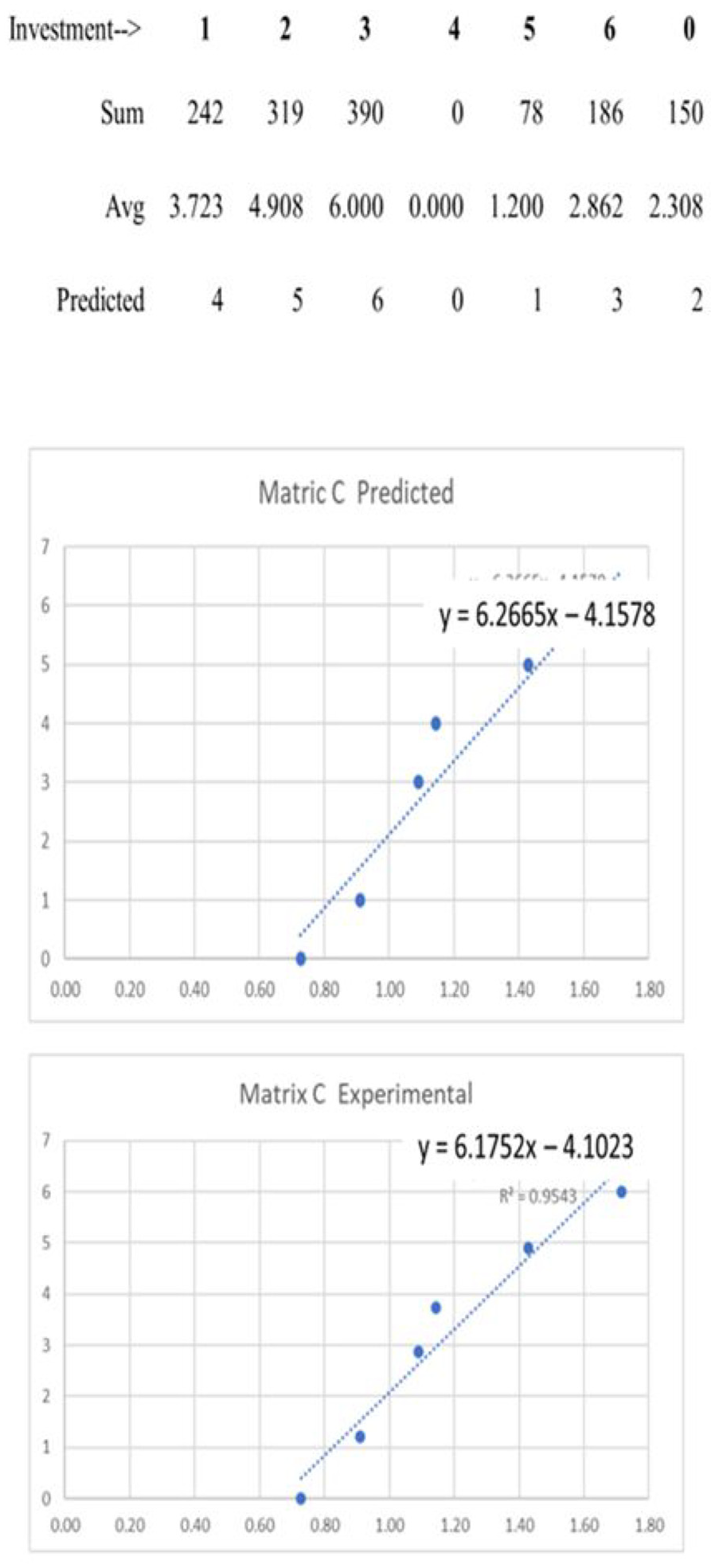
The experimental versus predicted rankings matrix C (N = 65).

The output matrix of ranked preferences for each respondent was then used to plot Ranking versus IRR:WACC Ratio for each individual respondent. A regressed line was fit to each, and the slope of each individual regressed line was calculated.

The slope (β) of the line that fits this data is statistically compared to the slope of the line that is predicted by the MIOS to test the following hypotheses (separately for each of the three maitrices):

H₀: β equals the slope of the line as predicted by the MIOS.

H_alt: β does not equal the slope of the line as predicted by the MIOS.

Respondents should be indifferent towards an investment when it has an IRR:WACC ratio of unity as this is the MIOS equilibrium point developed from EUT. However, in accordance with Prospect Theory, some people are risk averse and perceive losses and gains asymmetrically rather than linearly (Kahneman & Tversky, 1979; Tversky & Kahneman, 1986, 1991). To test this, Matrix A included a potential investment with an IRR:WACC ratio equal to unity as one of the treatments. In accordance with Prospect Theory, the survey data can be expected to show the MIOS equilibrium point positioned more conservatively (IRR:WACC > 1) than what would be predicted by EUT alone (IRR:WACC = 1). Its exact position is experiment-specific, cannot be known in advance, and is revealed through experiment (Tversky & Kahneman, 1986). Therefore, for Matrix A, a comparison was also made against the slope of the MIOS-predicted line incorporating Prospect Theory to test the following hypotheses:

H₀: β equals the slope of the line as predicted by the MIOS when incorporating Prospect Theory.

H_alt: β does not equal the slope of the line as predicted by the MIOS when incorporating Prospect Theory.

Statistical Analysis

The numerical values of these individually calculated slopes were populated into Excel CSV files for use in a statistical software package (JASP 18.1). A Shapiro-Wilks test indicated that this data was not normally distributed and was visually confirmed by looking at the Distribution plots and the Q–Q plots (Frost, 2020). A nonparametric test, such as the Wilcoxon signed rank test, is recommended when data is not normally distributed or when ordinal data is used (Frost, 2020; Harris & Hardin, 2013; Kitani & Murakami, 2022; Neuhäuser, 2015; Rosenblatt & Benjamini, 2018). Under instances of non-normality, the Wilcoxon signed rank test is more powerful than the t-test (Neuhäuser, 2015; Rosenblatt & Benjamini, 2018). Similarly, Kitani and Murakami (2022) provide an overview of various studies that indicate the Wilcoxon signed rank test shows increased performance over the t-test when normality cannot be assumed.

Furthermore, the calculated slopes of Ranking versus IRR:WACC Ratio are based on ordinal preference rankings. This results in a discrete set of possible values for the slopes, and this also points to the use of the nonparametric Wilcoxon signed rank test. Therefore, because of non-normality and because the paired comparison rankings are ordinal, the non-parametric Wilcoxon signed rank test was used to compare the experimentally derived slopes to the MIOS predicted slopes.

Findings

For Matrix A, the results of the Wilcoxon test suggest rejecting the null hypothesis for both boundary conditions, and thus conclude that 1) there is a significant difference (α = .05) between the slope of the experimentally calculated line and the slope of the predicted MIOS line, 2) there is a significant difference (α = .05) between the slope of the experimentally calculated line and the slope of the predicted MIOS line when incorporating risk aversion per Prospect Theory, and 3) these results provide statistical support that the slope of the experimentally calculated line lies between the boundary conditions of a) the slope of the predicted MIOS line and b) the slope of the predicted MIOS line when incorporating Prospect Theory. See Figure 7 which contains the statistical results including the p values. This is the expected outcome based on Prospect Theory, that is, that the experimental results would lie between the two boundary conditions. Therefore, this supports the prediction in section “Data reduction,” that the slope of the experimental line should fall somewhere between the two, and thus the MIOS accurately predicted the ranking of the project-financed investments.

Figure 7.

Wilcoxon test results for matrix A.

For Matrix B, the results of the Wilcoxon test suggest that the null hypothesis cannot be rejected (α = .05), and thus conclude that there isn’t a significant difference between the slope of the experimentally calculated line and the slope of the MIOS predicted line. See Figure 8 which contains the statistical results including the p values. This supports the prediction that the slope of the experimental line should equal that of the predicted line, and thus, as with Matrix A, the MIOS accurately predicted the ranking of the project-financed investments in Matrix B.

Figure 8.

Wilcoxon test results for matrix B.

For Matrix C, the Wilcoxon test suggests that the null hypothesis cannot be rejected (α = .05) and thus conclude that there is not a significant difference between the slope of the experimentally calculated line and the slope of the MIOS line. See Figure 9 which contains the statistical results including the p values. This test supports the prediction that the slope of the experimental line should equal that of the predicted line, and thus, as with Matrix A and Matrix B, the MIOS accurately predicted the ranking of the project-financed investments in Matrix C.

Figure 9.

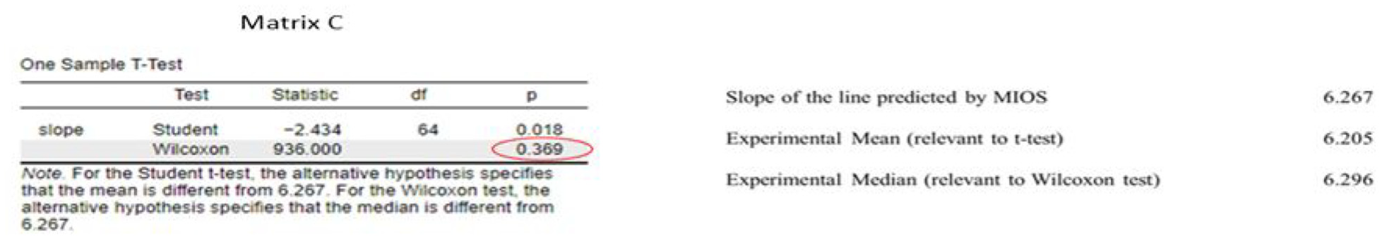
Wilcoxon test results for matrix C.

To summarize, the analysis was repeated using three different sets of 2 × 3 manipulations. Each time, statistical support was found for the MIOS as an appropriate method for ranking project-financed investments.

Observations Regarding the Data

Certain specific tests were designed into the manipulations. In Matrix A, one of the direct comparisons was between an investment having an IRR:WACC Ratio equal to unity (Investment #2; IRR = 10%; WACC = 10%) and the “no investment” choice. When the IRR equals the WACC, this is the MIOS-predicted equilibrium point in the absence of Prospect Theory. Prospect Theory states that some percentage of the respondents will select Investment #2 over the “no investment” option and some percentage, being those that are more risk-averse, will prefer the “no investment” option, thus pushing the experimental equilibrium point higher than IRR:WACC = 1.

The MIOS predicted that the experimental equilibrium point for the specific manipulations contained in Matrix A would lie somewhere between an IRR:WACC Ratio of 1.0 and 1.257. As noted previously, the exact percentage of respondents that will choose one way versus the other, and thus the exact location of the experimental equilibrium point, cannot be known in advance and is revealed through experiment (Tversky & Kahneman, 1986). The data for Matrix A shows that 80% (48 out of 60) of the respondents selected Investment #2 as their preference while 20% (12 out of 60) selected the more risk-averse choice of “no investment” per Prospect Theory. This resulted in an experimental equilibrium point of IRR:WACC = 1.062 which lies between the values of 1.0 and 1.257 as predicted by the MIOS.

In Matrix B, consistent with the MIOS predictions, the respondents presented clear preferences for investing in those projects with the higher IRR:WACC Ratios, clear preferences for those investments with IRR:WACC Ratios greater than unity, and a “no investment” preference for those projects with IRR:WACC Ratios less than unity.

Unlike Matrix B where the IRR:WACC choices were spread numerically further apart and perhaps easier for the respondents to mentally calculate while taking the survey, Matrix C contained a direct comparison where the IRR:WACC Ratios were close together. Specifically, the MIOS predicted that Investment #1 (IRR = 8; WACC = 7) with an IRR:WACC Ratio of 1.14 would be preferred over Investment #6 (IRR = 12; WACC = 11) with an IRR:WACC Ratio of 1.09. However, 13.8% (9 of 65) of the respondents selected Investment #6 over Investment #1 even though it had a slightly lower IRR:WACC Ratio.

This type of inconsistency tends to occur in paired comparison analyses when choices are close in value (Brown & Peterson, 2009; Choi et al., 2013; Johanson & Gips, 1993; Kingsley & Brown, 2010). This effect has been recorded as far back as Fechner in 1860 (Kingsley & Brown, 2010) and is attributed to the Law of Comparative Judgment which states that smaller degrees of “discriminal difference” increase the inconsistency of a test subject’s responses (Thurstone, 1994:266). Such is the case here where the choice was between two investments having IRR:WACC Ratios that were close together and the economic incentive for a respondent to complete a survey quickly was not aligned with completing the survey accurately.

Finally, each of the matrices included specific direct comparisons to determine if the respondents were making selections based on the IRR and not the IRR:WACC Ratio. There were eight such tests in total: Matrix A included two, and Matrices B and C each included three.

Without exception, all of the respondents in Matrix A and Matrix B made all their selections based on the IRR:WACC Ratio in support of the MIOS and not based on the IRR. However, in Matrix C, the responses were mixed. When the choice was between an IRR:WACC Ratio > 1 against an IRR:WACC Ratio <1, all of the respondents in Matrix C made their selection based on the IRR:WACC Ratio and not on the IRR. When both investments had an IRR:WACC Ratio > 1, and one ratio was significantly greater than the other, all but one person out of 65 chose the investment with the higher IRR:WACC Ratio. However, as discussed previously, when the IRR:WACC Ratios were close together (1.09 vs. 1.14) making it more difficult to ascertain which investment had the higher IRR:WACC Ratio without using a calculator, 13.8% (9 of 65) selected the investment with the higher IRR and not the higher IRR:WACC Ratio.

In summary, of the 495 selections involving the eight specific direct comparisons noted above, there were only 10 instances where a respondent selected the investment with the higher IRR rather than the higher IRR:WACC Ratio, and nine of these occurred when the IRR:WACC Ratios were close together. This represents a very high “coefficient of consistency” for a paired comparison analysis (Peterson & Brown, 1998). Thus, in general, it appears that respondents made their selections based on the IRR:WACC Ratio in support of the MIOS and not based on the IRR.

Calculation of the Experimental Equilibrium Point

To calculate the experimental equilibrium point, the experimentally derived average ranking for the “no investment” option (2.333 for Matrix A, 3.017 for Matrix B, and 2.308 for Matrix C) was inputted as “y” into the equation of the regressed line fitting the experimental data for each matrix. The equation of the regressed line for each matrix is provided in Figures 4 –6. This equation was solved for “x” which is the IRR:WACC Ratio that represents the experimental equilibrium point for each matrix. The results for each matrix are shown in Figures 10 –15.

Figure 10.

Matrix A: predicted ranking versus capital budget.

Figure 11.

Matrix A: experimental ranking versus capital budget.

Figure 12.

Matrix B: predicted ranking versus capital budget.

Figure 13.

Matrix B: experimental ranking versus capital budget.

Figure 14.

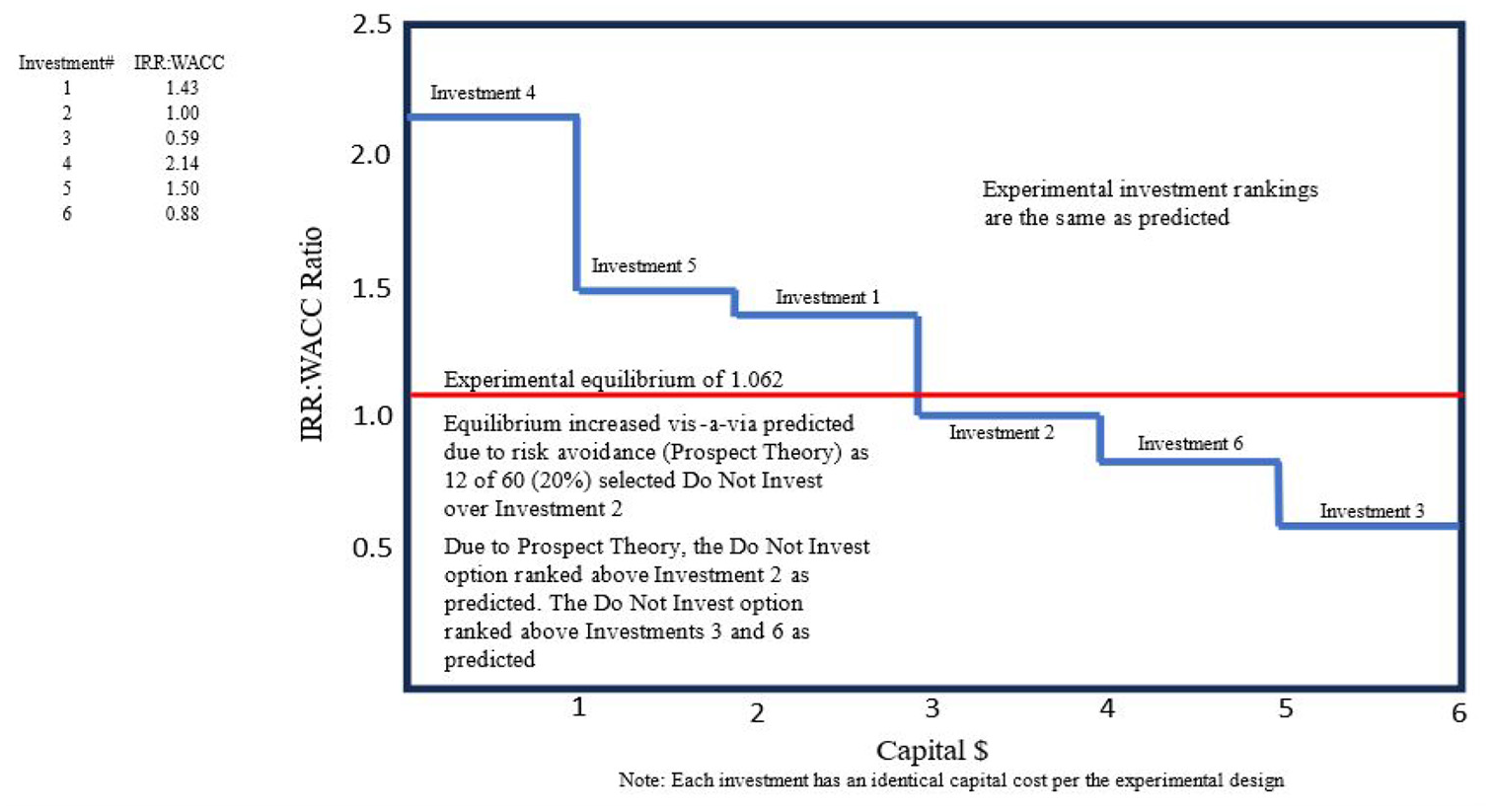
Matrix C: predicted ranking versus capital budget.

Figure 15.

Matrix C: experimental ranking versus capital budget.

These graphs are similar to those described by Coase (1937) to demonstrate his investment opportunity schedule (IOS) for balance sheet financing, except that the vertical axis is IRR:WACC in lieu of IRR. It is a key finding of this study that the specific rank ordering of the experimentally derived investment choices shown in Figures 10 –15 are identical to the predicted rank ordering, thus providing support for the MIOS ranking mechanism.

In Matrix A, as predicted, the experimentally derived equilibrium of IRR:WACC = 1.065 appears to show the impact of risk avoidance (Prospect Theory) as 20% (12 of 60) respondents selected the “no investment” option over Investment 2 (having an IRR:WACC Ratio = 1). In Matrix C, the experimentally derived equilibrium of 1.038 also appears to show the impact of risk avoidance as 32% (21 of 65) respondents selected the “no investment” option over Investment 6 (an IRR:WACC Ratio of 1.09) as well as 11% (7 of 65) selected the “no investment” option over Investment 1 (an IRR:WACC Ratio of 1.14). Evidence of risk avoidance did not appear in Matrix B likely because the numerical distance between Investment 1 (an IRR:WACC Ratio of 1.6) and the “no investment” option was too large. The data suggests that once the IRR:WACC Ratio reaches approximately 1.5, the expectation of profitable returns appears sufficient to overcome any risk aversion.

As shown in Figures 10 –15:

For all three matrices, the experimentally derived investment rankings are the same as the rankings predicted by the MIOS.

For all three matrices, the placement of the equilibrium point within the rankings is the same as predicted by the MIOS.

Therefore, all investments situated to the left of the equilibrium point should be internalized by the firm. Those situated to the right should remain external to the firm. In summation, quantitative support is found for the previously stated hypotheses:

H1: When making use of project financing, as opposed to balance sheet financing, the boundary or extent of the firm is established at an IRR:WACC ratio of unity.

Conclusions and Recommendations

Conclusions

This paper unearthed a theoretical assumption in Coase (1937) that limits the applicability of the Coasian IOS to balance-sheet financing. By shedding light on this limitation, this paper fills a gap in the literature by showing that the process by which economic utility theory gets applied to Internalization Theory is contingent on the method of financing. Coase’s underlying financing assumption causes the long-standing Investment Opportunity Schedule (IOS) to yield erroneous results when applied to project-financed investments.

The paper’s two hypotheses were supported, and the results suggest that the proposed new investment ranking mechanism, the MIOS, is the proper ranking mechanism for project-financed investment opportunities. Support for the new investment ranking mechanism is found using a paired comparison methodology which yields the ranking of the potential investments to be internalized as well as the placement of the equilibrium point. As shown in Figures 10 –15, the rankings for the various investments within the three matrices were as predicted by the MIOS and the locations of the equilibrium points were as predicted by the MIOS.

Finally, and perhaps most importantly for its theoretical implications, the answers to Coase’s two seminal questions (Which business opportunities should be internalized by a firm?, and What should be the extent or boundary of a firm?) are shown to be contingent on the method of financing. We now know that the Coasian IOS is not universal and cannot be used as the foundation for Internalization Theory studies that include any project-financed investments. Internalization Theory cannot stand on the IOS alone but requires a broader foundation. However, the IOS and MIOS, working in tandem, one for balance-sheet financing and one for project-financing, provide this broader foundation.

Practical Implications

This paper fills a 40-year gap in Internalization Theory literature by putting forth a new investment ranking mechanism, the MIOS, that is shown to be the proper ranking mechanism for project-financed investment opportunities. When project-financing is used, analysts should replace the IOS with the MIOS. This holds whenever project-financing is used and is independent of industry type (e.g., power plants, real estate, petroleum).

The MIOS provides financial decision-makers with a useful tool for corporate strategic planning to be used in parallel with the IOS; one tool for analyzing balance sheet investments and the other for project-financed investments. The IOS and the MIOS operate and function similarly, however, the assumption made by Coase in his development of the traditional IOS prevents it from being used for project-financed investments, and the assumptions used to develop the MIOS limit its use to project-financed investments. These underlying assumptions prevent either method from being used for the analysis of both types of financings.

Limitations

This paper made use of an experimental design analysis which provide high internal validity, replicability, and causality. The balanced PCBWS also increased internal validity by eliminating transitive assumptions, and the experiment increased validity through triangulation and parallel-form reliability. However, experimental design scenarios require respondents to imagine how they would react to stimuli that have been presented in a controlled format. Such data may not reflect real-life decision-making (Portney, 1994), and losing real money may lead to a different experimental outcome than losing hypothetical money (Bleichrodt & L’Haridon, 2023).

The manipulations selected for the analysis were selected to ensure that specific conditions were tested; specifically, combinations where the IRR:WACC ratio was less than, greater than, and equal to unity because the MIOS equilibrium point is equal to unity. The manipulations were not selected to reflect ecological validity.

For online surveys, the use of screener questions is considered best practice to ensure that respondents hold specific expertise, and this study’s screener questions were tested to be effective at weeding out those respondents who did not possess a certain level of financial expertise. However, the screener questions were not intended to guarantee that a respondent held a specific employment position. For this, our study relied on self-reported data.

Recommendations for Future Research

As noted previously, the demographic data was self-reported. It is recommended that the analysis be re-performed using participants whose credentials and experience can be verified through their place of employment.

The study made use of an experimental design analysis where the manipulations were varied at specific intervals to ensure that specific conditions were tested. Now that support for the model has been found, a follow-up study using manipulations having greater ecological validity can be performed. In addition, the analysis may be performed using actual investment data collected from corporations which would increase external validity, although we recognize the difficulty of obtaining the requisite data in a sufficiently large quantity to support a quantitative analysis.

Recommendations for Past Research

Given the very large size of the global project-financing market, and given the now-exposed critical difference between the rival assumptions of balance-sheet and project-financing and the effect of these assumptions on internalization outcomes, Internalization Theorists may wish to review whether their data sets comingled balance-sheet and project-financed investments because any co-mingling may have affected the validity of their research. Specifically, the outcomes of past research may be based on data which include project-financed investments for which the traditional IOS does not apply, and as shown herein, the co-mingling of balance-sheet and project-financed data yields erroneous results.

Footnotes

ORCID iD

Stephen Dansky

Ethical Considerations

The research protocol was reviewed and approved by the Florida Institute of Technology IRB (Date: May 18, 2023; IRB Number: 23-072), and voluntary informed consent was provided by each survey participant. Finally, artificial intelligence (AI) was not used for the research and authorship of this article.

Funding

The author(s) received no financial support for the research, authorship, and/or publication of this article.

Declaration of Conflicting Interests

The author(s) declared no potential conflicts of interest with respect to the research, authorship, and/or publication of this article.

Data Availability Statement

Data sharing not applicable to this article as no datasets were generated or analyzed during the current study.

References

Auger

Devinney

Louviere

(2007). Using best–worst scaling methodology to investigate consumer ethical beliefs across countries. Journal of Business Ethics, 70(3), 299–326.

Baldauf

Jochem

(2024). Project finance or corporate finance for renewable energy? An agent-based insight. Journal of Economic Interaction and Coordination, 19, 759–805. https://doi.org/10.1007/s11403-024-00425-z

Bansal

(2017). Survey sampling. Alpha Science International Limited.

Baumol

W. J.

Malkiel

B. G.

(1967). The firm’s optimal debt-equity combination and the cost of capital. The Quarterly Journal of Economics, 81(4), 547–578. https://doi.org/10.2307/1885578

Berinsky

Margolis

Sances

(2014). Separating the shirkers from the workers? Making sure respondents pay attention on self-administered Surveys. American Journal of Political Science, 58(3), 739–753.

Bardsley

Cubitt

Loomes

Moffatt

Starmer

Sugden

(2010). Experimental economics: Rethinking the rules. Princeton Univ. Press.

Bleichrodt

L’Haridon

(2023). Prospect Theory’s loss aversion is robust to stake size. Judgment and Decision Making, 18(e14), 1–21. https://doi.org/10.1017/jdm.2023.2

Bougie

Sekaran

(2020). Research methods for business: A skill building approach, 8th ed. Wiley.

Brigham

E. F.

(1979). Financial management: Theory and practice (2 ed.). Dryden Press.

10.

Brigham

E. F.

Ehrhardt

M. C.

(2017). Financial Management: Theory and Practice, 15th ed. Cengage.

11.

Brown

T. C.

Peterson

G. L.

(2009). An enquiry into the method of paired comparison: Reliability, scaling, and Thurstone’s law of comparative judgment. United States Department of Agriculture, Rocky Mountain Research Station, General Technical Report RMRS-GTR-216WWW, 98p.

12.

Buckley

P. J.

(1988). The limits of explanation: Testing the internalization theory of the multinational enterprise. Journal of International Business Studies,19(2), 181-191.

13.

Buckley

P. J.

Casson

M. C.

(2009). The internalization theory of the multinational enterprise: A review of the progress of a research agenda after 30 years. Journal of International Business Studies, 40(9): 1563–1580.

14.

Buscaino

Caselli

Corielli

Gatti

(2012). Project finance collateralised debt obligations: An empirical analysis of spread determinants. European Financial Management, 18(5), pp.950–969. https://doi.org/10.1111/j.1468-036X.2010.00560.x

15.

Caves

R. E.

(1996). Multinational enterprise and economic analysis, 2nd ed. Cambridge University Press.

16.

Choi

K.C.

W.K.W.

P. W.C.

Lau

S.F.

J.C.K.

(2013). Consistency in paired comparisons of information needs questionnaires (INQ) among Hong Kong Chinese breast cancer patients. European Journal of Oncology Nursing, 17, 170-175.

17.

Clifford

P. D.

(2020). Project finance: Applications and insights to emerging markets infrastructure. Wiley & Sons. https://ebookcentral.proquest.com/lib/fit/detail.action?docID=6380283.

18.

Coase

R. H.

(1937). The nature of the firm. Economica, 4(16), 386–405. https://doi.org/portal.lib.fit.edu/10.2307/2626876

19.

Cohen

Orme

(2004). What’s your preference? Marketing Research, 16(2), 32–37.

20.

Danilova

Horstmann

Smith

Naiakshina

(2022). Testing Time Limits in Screener Questions for Online Surveys with Programmers. In International Conference on Software Engineering (ICSE ’22), May 21–29, 2022, Pittsburgh, PA, USA. https://doi.org/10.1145/3510003.3510223

21.

DeSimone

Harms

(2017). Dirty data: The effects of screening respondents who provide low-quality data in survey research. Journal of Business Psychology, 33, 559–577. https://doi.org/10.1007/s10869-017-9514-9

22.

DeSimone

Harms

DeSimone

(2015). Best practice recommendations for data screening. Journal of Organizational Behavior, 36, 171–181. https://doi.org/10.1002/job.1962

23.

Fight

(2006). Introduction to project finance. Butterworth-Heinemann.

24.

Frost

(2020). Hypothesis Testing. Statistics by Jim Publishing.

25.

Furlan

Turner

(2014). Maximum difference scaling. International Journal of Market Research, 56(3), 367–385.

26.

Gamel

Menrad

Decker

(2016). Is it really all about the return on investment? Exploring private wind energy investors’ preferences. Energy Research & Social Science, 14, 22-32. https://doi.org/10.1016/j.erss.2016.01.004

27.

Harris

Hardin

(2013). Exact Wilcoxon signed-rank and Wilcoxon Mann–Whitney rank sum tests. The Stata Journal, 13(2), 337–343

28.

Hawkins

G. E

Marley

A. A. J

Heathcote

Flynn

T. N.

Louviere

J. J.

(2014). The best of times and the worst of times are interchangeable. Decision, 1(3), 192–214. https://doi.org/10.1037/dec0000012

29.

Hennart

J-F.

(1988). A transaction costs theory of equity joint ventures. Strategic Management Journal, 9(4), 361–374.

30.

Jadidi

Firouzi

Rastegar

M. A.

Zandi

(2020). Bayesian updating of solar resource data for risk mitigation in project finance. Solar Energy, 207, 1390–1403.

31.

Johanson

G. A.

Gips

C. J.

(1993). Paired comparison intransitivity: Useful information or nuisance?Annual Meeting of the American Educational Research Association.

32.

Kahneman

Tversky

(1979). Prospect theory: An analysis of decision under risk. Econometrica, 47, 263–291. https://doi.org/10.2307/1914185

33.

Kaminker

C. R.

(2017). The role of institutional investors in financing sustainable energy. PhD Dissertation, University of Oxford, Kellogg College.

34.

Kay

(2015). Coase and the contribution of ‘The Nature of the Firm’. Managerial and Decision Economics, 36, 44–54.

35.

Kingsley

D. C.

Brown

T. C.

(2010). Preference uncertainty, preference learning, and paired comparison experiments. Land Economics, 86(3), 530–544.

36.

Kingsley

D. C.

Brown

T. C.

(2013). Estimating willingness to accept using paired comparison choice experiments: Tests of robustness. Journal of Environmental Economics and Policy, 2(2), 119–132. DOI: 10.1080/21606544.2013.775602

37.

Kitani

Murakami

(2022). One-sample location test based on the sign and Wilcoxon signed-rank tests. Journal of Statistical Computation and Simulation, 92(3), 610–622. https://doi/org/10.1080/00949655.2021.1968399

38.

Klompjan

Wouters

(2002). Default risk in project finance. The Journal of Structured Finance, 8(3), 10-21.

39.

Lee

J. A.

Soutar

G. N.

Louviere

(2007). Measuring values using best-worst scaling: The LOV example. Psychology & Marketing, 24(12), 1043-1058.

40.

Lehmann

Erich

. (2011). Fisher, Neyman, and the creation of classical statistics.

41.

Levin

I. P.

(1999). Relating statistics and experimental design: An introduction. Quantitative applications in the social sciences (Vol. 125). SAGE Publications, Inc.

42.

Louviere

J. J.

Islam

(2008). A comparison of importance weights and willingness-to-pay measures derived from choice-based conjoint, constant sum scales and best-worst scaling. Journal of Business Research, 61, 903–911. https://doi.org/10.1016/j.jbusres.2006.11.010

43.

Mahajan

Green

Goldberg

(1982). A conjoint model for measuring self-and cross-price/demand relationships. Journal of Marketing Research, 19(3), 334–342.

44.

Marley

A. A. J.

Louviere

J. J.

(2005). Some probabilistic models of best, worst, and best–worst choices. Journal of Mathematical Psychology, 49(6), 464–480. https://doi/org/10.1016/j.jmp.2005.05.003

45.

Massey

G.R.

Wang

P. Z.

Waller

D.S.

Lanasier

E.V.

(2015). Best–worst scaling: A new method for advertisement evaluation. Journal of Marketing Communications, 21(6), 425–449. https://doi/org/10.1080/13527266.2013.828769

46.

Mora

Spelling

van der Weijde

Pavageau

E-M.

(2019). The effects of mean wind speed uncertainty on project finance debt sizing for offshore wind farms. Applied Energy, 252, 113419. https://doi.org/10.1016/j.apenergy.2019.113419

47.

Narula

Asmussen

C. G.

Chi

Kundu

S. K.

(2019). Applying and advancing internalization theory: The multinational enterprise in the twenty-first century. Journal of International Business Studies, 50(8), 1231–1252. https://doi/org/10.1057/s41267-019-00260-6

48.

Nermend

Latuszynska

(2016). Selected issues in experimental economics. Proceedings of the 2015 Computational Methods in Experimental Economics (CMEE) Conference. Springer, 385 pp.

49.

Neuhäuser

(2015) Combining the t test and Wilcoxon’s rank-sum test. Journal of Applied Statistics, 42(12), 2769-2775. https://doi/org/10.1080/02664763.2015.1070809

50.

Nobel (2023). The Sverges Risbank prize in economic sciences in memory of Alfred Nobel. The Nobel Prize. Retrieved February 6, 2023, from https://www.nobelprize.org/prizes/economic-sciences/

51.

Peterson

Brown

(1998). Economic valuation by the method of paired comparison, with emphasis on evaluation of the transitivity axiom. Land Economics, 74(2), 240–261.

52.

Portney

P. R.

(1994). The contingent valuation debate: Why economists should care. Journal of Economic Perspectives, 8(4): 3–17. https://doi/org/10.1257/jep.8.4.3

53.

Rausch

T. M.

Baier

Wening

(2021). Does sustainability really matter to consumers? Assessing the importance of online shop and apparel product attributes. Journal of Retailing and Consumer Services, 63, 1–16. https://doi.org/10.1016/j.jretconser.2021.102681

54.

Refinitiv (2024). Global project finance review full year 2022. Retrieved November 5, 2024, from https://www.lseg.com/en/data-analytics/reports-2022-q4-global-project-finance-review.pdf

55.

Rosenblatt

Benjamini

(2013). Another argument in favour of Wilcoxon’s Signed Rank test. arXiv:1311.5354v1, https://doi.org/10.48550/arXiv.1311.5354

56.

Ross

S. A.

Modigliani

Westerfield

R. W.

(2016). Fundamentals of corporate finance, 11th ed. Richard D. Irwin, Inc. Publishers,

57.

Rugman

A. M.

(1986). New theories of the multinational enterprise: An assessment of internalization theory. Bulletin of Economic Research, 38(2), 101–118.

58.

Samarzija

N. D.

(2019). Determining the marginal willingness to pay for the cervical cancer screening program in Croatia: A best-worst scaling approach. Society and Economy, 41(4), 433–447. https://doi/org/10.1556/204.2019.016

59.

Sharpe-Wessling

Huber

Oded

(2017). MTurk character misrepresentation: –Assessment and solutions. Journal of Consumer Research, 44(1), 211–230. https://doi/org/10.1093/jcr/ucx053

60.

Strickland

Stoops

(2020). Utilising content-knowledge questionnaires to assess study eligibility and detect deceptive responding. The American Journal of Drug and Alcohol Abuse, 46(2), 149–157. https://doi.org/10.1080/00952990.2019.1689990

61.

Tanaka

Nelson

McCullar

Parulekar

(2022). Citizens’ preferences on green infrastructure practices and their enhancement in Portland, Oregon. Journal of Environmental Management, 318, 1–13. https://doi.org/10.1016/j.jenvman.2022.115415

62.

Thurstone

L. L.

(1994). A law of comparative judgment. Psychological Review, 101(2), 266–270. https://doi.org/10.1037/0033-295X.101.2.266

63.

Toich

Schutt

Fisher

(2021). Do you get what you pay for? Preventing insufficient effort responding in MTurk and student samples. Applied Psychology, 71, 640–661. https://doi/org/10.1111/apps.12344

64.

Tversky

Kahneman

(1986). Rational choice and the framing of decisions. Journal of Business, 59(4), 251–278.

65.

Tversky

Kahneman

(1991). Loss aversion in riskless choice: A reference-dependent model. The Quarterly Journal of Economics, 106(4), 1039–1061. https://doi.org/10.2307/2937956

66.

Ugboma

(2021). Developing sustainable energy projects in emerging markets. Business Expert Press.

67.

USDA (2023). The method of paired comparisons. Retrieved February 14, 2023, from https://www.fs.usda.gov/rmrs/method-paired-comparisons.

68.

Verbeke

(2005). Internalization, international diversification and the multinational enterprise. JAI Press.

69.

Verbree

Toepoel

Perada

(2020). The effect of seriousness and device use on data quality. Social Science Computer Review, 38(6), 720–738. https://doi/org/10.1177/0894439319841027

70.

Williamson

O.E.

(1975). Markets and hierarchies: Analysis and antitrust implications: A study in the economics of internal organizations. Free Press, Macmillan, New York.

71.

Yescombe

E. R.

(2002). Principles of project finance. Academic Press.

Rethinking Internalization Theory due to Coase’s “Hidden in Plain Sight” Assumption

Abstract

Plain Language Summary

Keywords

Introduction

Conceptual Development

Internalization Theory

The Change from Balance Sheet to Project Financing

Identification of the Problem

The Modified IOS

The View from the Perspective of the Investing Company

Methodology

Ranked Preferences Methods for Experimental Analyses

PCBWS Experimental Manipulations

Experimental Validity

Findings and Data Analysis Results

Description of the Survey Instrument and Data Collection

Demographics

Data Reduction

Statistical Analysis

Findings

Observations Regarding the Data

Calculation of the Experimental Equilibrium Point

Conclusions and Recommendations

Conclusions

Practical Implications

Limitations

Recommendations for Future Research

Recommendations for Past Research

Footnotes

ORCID iD

Ethical Considerations

Funding

Declaration of Conflicting Interests

Data Availability Statement

References