Sage Journals: Discover world-class research

Abstract

There has always been a pressing need to provide semantic information for words in high-frequency word lists, but technical limitations have hindered this goal. This study addresses this challenge by leveraging a large language model, such as BERT, to semantically annotate large corpora and identify the high-frequency senses of headwords from the General Service List (GSL). We aim to explore three key questions: (1) Can BERT automatically annotate large corpora and accurately calculate sense frequencies? (2) What are the high-frequency senses of GSL words? (3) Can this approach be verified? Using a BERT-based framework, we annotated 1,891 GSL headwords (10,925 senses) in the 100-million-word British National Corpus (BNC), representing each sense with a 1,024-dimensional vector. From this, we identified 3,695 high-frequency senses for the GSL words. Three main conclusions are drawn from this study. First, BERT demonstrates high accuracy in sense annotation, achieving 92% precision when disambiguating the senses of GSL words. Second, a relatively small number of high-frequency senses account for a significant portion of corpus coverage. Specifically, these high-frequency senses (33.8% of the total) cover approximately 60% of all GSL word occurrences in the BNC. Third, the high-frequency senses selected via this method can be verified by their consistent coverage across different corpora. This study illustrates a pioneering method for semantic annotation in large corpora, which can be easily applied to calculate semantic frequencies for other word lists.

Plain language summary

Understanding common word meanings: Using large language model to analyze word frequency

This research utilizes a BERT model to analyze how often different meanings of common words, listed in the General Service List (GSL), appear in large collections of texts. By assigning a numerical value to each meaning, the study calculates their frequency in the British Nation Corpus (BNC). It finds that a small number of meanings cover a large portion of text, suggesting their importance for language learners. The study also reveals consistent usage patterns across different time periods, providing valuable insights for language teaching and learning.

Keywords

word lists semantic annotation semantic frequency BERT large language model

Introduction

For beginners learning a foreign language, it is out of the question to master every word of it due to the vastness of the vocabulary of most languages. Instead, they are advised to optimize their learning by concentrating on the high-frequency words first (Nation, 2016). Consequently, several high-frequency word lists have been created.

One of the most influential lists is West’s (1953)“A General Service List of English Words” (GSL). It has served as the foundation for the development of new word lists (Brezina & Gablasova, 2015; Coxhead, 2000), a standard for evaluating lexical suitability in learning materials (C. Y. Liu, 2023; Vuković-Stamatović, 2022), as well as a guide for vocabulary learning (Vilkaitė-Lozdienė & Schmitt, 2020). Although created in the 1950s, it remains among the best word lists available (Schmitt & Schmitt, 2020).

One important reason for its lasting influence is that the GSL provides information about the frequency of each word’s meanings (Nation & Waring, 1997). Beyond simply listing the spelling forms, it explicitly describes various senses and sense frequencies. For example, it not only identifies that “capital” is a commonly used English word, but also emphasizes that its “city” sense is significantly more prevalent than its “letter” sense. As explicitly stated in the GSL, 47% of the instances of “capital” are associated with the meaning of “city,” while only 1% of the occurrences are related to the meaning of “letter” (West, 1953: 69). Likewise, the GSL indicates that “air” is a common word, but its use in the sense of “manner” represents only 5% of all cases. This particular meaning is enclosed in square brackets in the GSL, indicating that it is not widely used or recommended for teaching (West, 1953: 13).

Such semantic information is particularly valuable for language learners using these word lists. Since many English words are polysemous, learners or even teachers often find it challenging to determine which meaning(s) to focus on when consulting these lists. If we acknowledge that high-frequency words should be learned first, then high-frequency senses should also receive early attention, with less frequent senses saved for later study. As pointed out by West (1953), although “air” is a common word, its meaning of “manner” might not be crucial for younger learners. If we want to prioritize frequent senses over rarer ones, one critical question arises: how do we identify which senses are most common?

Different efforts have been made to update the GSL in recent years. Notable recent word lists include Nation’s (2012) BNC/COCA List, Browne et al. (2013) New General Service List (NGSL), Brezina and Gablasova’s (2015) New General Service List (New-GSL), and Schmitt et al.’s (2021) Knowledge-based Vocabulary Lists (KVL). These new lists have never tried to provide any semantic information for their selected words.

Semantic frequency information, which is absent in existing word lists, cannot be found in English dictionaries either. English dictionaries frequently stress the importance of ranking senses in order of frequency. Cambridge Learners’ Dictionary explicitly stated that the “most common meaning” was featured first in their entries. Oxford Learners’ Dictionary stated that the different meanings of a word were usually given in order of frequency, with the most frequent meaning given first. Longman Dictionary of Contemporary English upheld a similar frequency-based principle, stating that “meanings are organized by frequency.” Despite similar claims, it is interesting to note that different dictionaries arrange the senses in quite different orders. It is hard to tell which dictionary is correct because no dictionary provides detailed data on semantic frequency.

Semantic frequency has not been adequately calculated mainly due to methodological constraints. While current corpora techniques allow us to count word forms easily, they are unable to distinguish different senses. In West’s time, the semantic frequency was manually counted. However, as modern corpora become increasingly large, manual counting of 10,000 senses of approximately 2,000 words in a large corpus becomes practically impossible. Fortunately, the large language models that appeared in recent years provide a possible way to explore semantic frequency.

In this article, we will use Bidirectional Encoder Representations from Transformers (BERT), a large language model developed by Google, to calculate the semantic frequency of the GSL words in modern English corpora. This will involve annotating corpora semantically, selecting high-frequency senses, checking their coverage, and ultimately discussing theoretical implications. The method of calculating the semantic frequency of the GSL words in the BNC, as will be discussed later, can be easily applied to calculate the semantic frequency for any word list.

This study is guided by three research questions designed to address the methodological and pedagogical gaps in semantic frequency analysis:

(1) Can BERT automatically annotate large corpora and accurately calculate sense frequencies? (Addressed in Section 4.1: Semantic Frequency of GSL Words and Annotation Accuracy)

(2) What are the high-frequency senses of GSL words? (Addressed in Section 4.2: Selection of High-frequency Senses)

(3) Can this approach be justified? To be specific, can these senses achieve similar coverage with much fewer items than previous lists, and can they remain stable across various corpora? (Addressed in Section 4.3: Verification of Selected Senses)

By systematically answering these questions, this study, by demonstrating how to identify high-frequency senses of the GSL words, introduces a replicable framework for calculating semantic frequency in large corpora automatically.

Literature Review

Since the creation of the GSL, several updated word lists, including New-GSL and NGSL, have been developed. In this section, we will examine the progress made by these new lists as well as the challenges they face. We will also review the main methods for semantic annotation used in previous studies.

Previous Development of General Service Word Lists

West’s (1953) GSL is a list of about 2,000 words considered suitable as the basis for learning English as a foreign language. These words are organized alphabetically and include concise definitions as well as example sentences. Each word is assigned a number indicating how many times it appears in a corpus of 5 million words. What is more important, semantic frequency is provided for each meaning. GSL has had a wide influence for many years.

Despite its impact, GSL has faced criticism for being outdated and for its conflicting selection criteria. Richards (1974) argued that GSL no longer met contemporary instructional needs, as language use has changed since the creation of GSL in the first decades of the 20th century. Additionally, the challenges of expanding or updating the GSL were highlighted in several studies (Brezina & Gablasova, 2015; Gilner & Morales, 2008). In addition to the quantitative measure of word frequency, West (1953) also used some qualitative criteria, including ease of learning, necessity, cover, and stylistic and emotional neutrality (West, 1953: ix–x). Brezina and Gablasova (2015) pointed out that there was a strong tension between the quantitative and the qualitative principles, and some of the principles were highly subjective and dependent on the compiler’s preferences.

In response to these criticisms, two updated GSL lists, both titled the New General Service List, have been developed. To distinguish between them, the list created by Brezina and Gablasova (2015) is frequently referred to as New-GSL, while the one compiled by Browne et al. (2013) is referred to as NGSL.

Brezina and Gablasova (2015) used a combination of three quantitative measures: frequency, dispersion, and distribution. No subjective criteria were used. The New-GSL includes a total of 2,494 lemmas and achieves similar coverage to the original GSL. This list covers about 80% of the texts in BNC. This marks a significant reduction from the 4,100 lemmas required by West’s GSL to achieve comparable coverage.

The NGSL, developed by Browne et al. (2013), expanded and refined West’s GSL. First created in 2013 from a 273 million-word subset of the Cambridge English Corpus, it has been updated in 2016 and 2023. The 2,809 words of the NGSL offer more coverage with fewer words than the original GSL. It gives an average of 92% coverage of most texts of general English and even higher coverage in other situations. According to the authors’ official website, NGSL contains the most essential words for everyday English and is particularly beneficial for second language learners.

In addition to the two lists called New General Service Lists, many other high-frequency word lists have been created, including Davies and Gardner’s (2010) A Frequency Dictionary of Contemporary American English and Nation’s (2012) BNC/COCA List. Although these lists have different names, they are developed using similar principles and serve comparable purposes to GSL.

These recent word lists are based on large and contemporary corpora, but none provides information about sense frequency information. Regrettably, GSL is still the only high-frequency word list that provides semantic frequency. The lack of progress is mainly due to technical constraints.

Previous Methods of Calculating Sense Frequency

While traditional and semi-automated approaches have laid the foundation for sense frequency analysis, their reliance on manual annotation, rule-based systems, or shallow statistical methods has limited their scalability and adaptability to diverse linguistic contexts. Early methods, such as those based on WordNet (Miller, 1995) or corpus-based frequency counts, provided valuable insights into lexical semantics but struggled to capture the nuanced, context-dependent nature of word senses. These limitations became increasingly apparent with the growing complexity of natural language data and the demand for more robust, automated solutions. The advent of neural language models, particularly BERT (Devlin et al., 2018), marked a paradigm shift in semantic analysis by leveraging deep learning to model contextualized word representations. This section first reviews traditional and semi-automated approaches (Section 2.2.1), followed by a detailed discussion of how neural language models, especially BERT, have addressed the shortcomings of earlier methods (Section 2.2.2).

Traditional and Semi-Automated Approaches

Previous studies of sense frequency have relied on manual counting or semi-manual counting until the recent development of large language models such as BERT.

Traditionally, sense frequencies are manually counted. To obtain the semantic frequency of GSL words, the 13-volume of the Oxford English Dictionary (OED) was split into folios of 32 pages. Each person doing the counting was specially trained. He read the materials and whenever he found a word in his section of the dictionary he made a record of it. He then studied its apparent meaning in the context to assign its proper meaning. Each person doing the counting usually read all of the 5 million words. This approach is labor-intensive and time-consuming.

The advancement of modern corpora has simplified this procedure. Thanks to modern corpus techniques, researchers can now retrieve concordance lines containing specific words much more easily than before. However, sense annotation still requires manual effort. Due to the large volume of instances, it is impossible to analyze every one in detail. As a common practice, researchers typically analyze only a subset of instances, which are selected either randomly or through systematic sampling methods. Lin and Wang (2019) investigated the semantic changes of the adverb “again.” After gathering all instances of “again” from the Corpus of Historical American English (COHA), they randomly selected 479 samples at a ratio of 600:1 for manual annotation.

In recent years, many new approaches to identifying the correct meaning of words in large corpora have been proposed. They can mainly be divided into two groups: supervised methods (Iacobacci et al., 2016; Melamud et al., 2016; Raganato et al., 2017a; Yuan et al., 2016; Zhong & Ng, 2010) and knowledge-based methods (Agirre & Soroa, 2009; Luo et al., 2018; Moro et al., 2014; Raganato et al., 2017b). Supervised methods perform better than knowledge-based methods, but they need large sense annotated corpora first, while knowledge-based methods are usually unsupervised and require no sense annotated data. The accuracy of knowledge-based methods is generally around 65%, while that of supervised methods is around 70%. Although this level of accuracy is useful for preliminary exploration and research, it is indeed insufficient to support applications that require high precision, such as semantic annotation.

Neural Language Models and BERT Breakthroughs

With the introduction of deep neural network-based language models like ELMo (Peters et al., 2018), GPT (Radford et al., 2018), and BERT (Devlin et al., 2018), dynamic representations of words became feasible. These models compute different vectors for a target word based on the specific context, enabling the word vectors to express the commonalities and individualities of words in different contexts. In computational linguistics, a vector representation translates linguistic units (words, phrases, or senses) into numerical arrays, enabling machines to process semantic relationships. For instance, the word “king” might be represented as [0.71, −0.32, 0.45,…], where each dimension captures latent features like gender (“king” vs. “queen”) or royalty (“king” vs. “commoner”). BERT generates such vectors dynamically based on context—for example, “bank” in “river bank” versus “bank account” receives distinct vectors. In the vector space, words with similar meanings tend to cluster together, allowing for the computation of similarities and differences between words through mathematical operations.

Of these models, BERT performs better at distinguishing different meanings. As shown in Figure 1, BERT relies on a bidirectional multi-layer Transformer (Vaswani et al., 2017) to enable bidirectional context interaction. The Transformer architecture is entirely based on self-attention mechanisms, as opposed to the recurrent neural networks (RNNs) and convolutional neural networks (CNNs) commonly used in sequence modeling. The self-attention mechanism is designed to consider various positions within a sequence simultaneously to capture its representation. OpenAI’s GPT uses a unidirectional Transformer from left to right, while ELMo combines independently trained left-to-right and right-to-left Long Short-Term Memory networks (LSTMs). Among these models, only BERT’s representation is determined by the context from both the left and right across all layers. This approach revolutionized the conventional left-to-right computation methods used in earlier text analysis and representation models.

Figure 1.

Differences in pre-trained model architectures (Devlin et al., 2018).

As depicted in Figure 2, the input to the BERT model consists of three parts: token embeddings, segment embeddings, and position embeddings. The special token [CLS] represents the initial token and can symbolize the entire sentence. The special token [SEP] is used at the end of a sentence, enabling the generation of separate segment embeddings for two sentences, thus allowing the model to handle inter-sentence relationships. The word “playing” is split into “play” and “##ing” due to the WordPiece algorithm (Wu et al., 2016). Segment embeddings differentiate between different sentences, with the first sentence in the diagram having the segment embedding EA and the second sentence having EB. Position embeddings represent different position information.

Figure 2.

BERT input representation (Devlin et al., 2018).

During the pre-training phase, BERT employs two tasks: the masked language model (MLM) task and the next sentence prediction (NSP) task. The MLM task is akin to cloze tests in examinations where a sentence is given with one or more words being randomly masked, and the model predicts the masked words based on the remaining vocabulary. The NSP task involves determining whether an ensuing sentence in the same corpus is the right one to follow the first, a binary classification task with possible answers of yes or no. This task resembles paragraph ordering questions seen in examinations. The pre-training process of BERT, which combines both tasks, allows the model to learn vocabulary-related knowledge through the MLM task and acquire sentence-to-paragraph-level semantic information through the NSP task. The combined tasks enable the model’s word vectors to depict the input text’s information as comprehensively and profoundly as possible. Pre-training essentially involves continuously adjusting the model parameters to enhance the model’s understanding of language.

Many scholars have found through probing tasks that BERT word vectors encode multiple levels of linguistic knowledge. For instance, Tenney et al. (2019) demonstrated that BERT’s layers capture hierarchical linguistic features, with lower layers encoding syntactic information and higher layers focusing on semantic understanding. Similarly, N. F. Liu et al. (2019) showed that BERT effectively models syntactic dependencies, such as part-of-speech tagging and parsing. Goldberg (2019) further confirmed BERT’s capability to handle subject-verb agreement, a key syntactic phenomenon. Additionally, Ettinger (2020) revealed that BERT can represent semantic roles, though it struggles with more complex linguistic phenomena.

In parallel, researchers have fine-tuned BERT and tested its performance on word sense disambiguation (WSD) tasks across different languages. Huang et al. (2019) achieved 77.0% accuracy on WSD datasets using BERT-based model, outperforming traditional LSTM-based models (68.4%). Wiedemann et al. (2019) demonstrated that BERT achieves state-of-the-art results in SensEval-2 and SensEval-3 WSD tasks, outperforming traditional models. Du et al. (2019) fine-tuned BERT on WSD tasks, demonstrating BERT’s powerful capabilities in WSD and proving that incorporating external knowledge (such as sense definitions) can significantly enhance model performance. Wang and Wang (2020) proposed a novel Synset Relation-Enhanced Framework approach to optimize sense embeddings, further improving BERT’s WSD performance. Pawar et al. (2021) addressed the challenges of WSD in low-resource languages, leveraging BERT’s transfer learning capabilities. Loureiro et al. (2021) highlighted BERT’s limitations in handling low-frequency senses, while still acknowledging its overall effectiveness in WSD tasks. Finally, X. Zhou et al. (2024) extended BERT’s application to cross-lingual semantic analysis, demonstrating its potential to handle semantic shifts across languages.

BERT has also been applied to diachronic semantic analysis, which involves tracking semantic changes over time. Beck (2020) proposed a novel approach leveraging pre-trained BERT to generate contextualized word embeddings for Task 1 of SemEval-2020, a lexical semantic change task proposed by Schlechtweg et al. (2020), demonstrating that the system effectively detects semantic shifts in English, German, Latin, and Swedish with an accuracy of 0.728. W. Zhou et al. (2023) empirically demonstrated that enhancing contextual models through fine-tuning tasks significantly improves their effectiveness in detecting semantic change. The integration of multiple linguistic information in fine-tuning tasks notably enhances model performance, particularly when processing historical texts. This finding provides a new direction for future semantic change research and underscores the importance of incorporating rich linguistic information into models.

BERT’s Impact on Lexical Semantic Analysis

The model’s ability to capture sense-specific frequencies operationalizes call for usage-based lexical prioritization (D. Gardner, 2007; Nation, 2001; Schmitt, 2010). These theoretical and practical advancements highlight BERT’s potential to bridge the gap between computational linguistics research and applied language pedagogy. However, despite its success in semantic analysis, BERT’s application in pedagogical lexicography remains underexplored, particularly in the context of second language (L2) vocabulary instruction.

While BERT has demonstrated remarkable performance in tasks such as word sense disambiguation and semantic similarity, its direct application to pedagogical lexicography faces several challenges. First, BERT’s embeddings are computationally intensive and require significant resources for fine-tuning and deployment. Second, its sense representations, though contextually rich, may not align with the specific needs of L2 learners, such as stylistic appropriateness or frequency-based prioritization. Third, existing methods for semantic frequency analysis often lack scalability and replicability, limiting their utility in large-scale pedagogical contexts.

To address these challenges, our study innovates by:

(1) Scaling BERT to pedagogical lexicography through sense vector averaging (cf. Section 3.2.1). By aggregating BERT’s contextualized embeddings, we create robust sense representations that capture both frequency and semantic nuances, enabling more accurate and efficient vocabulary analysis.

(2) Introducing OED-based stylistic filtering for L2 relevance (cf. Table 3). We integrate stylistic annotations from the Oxford English Dictionary to ensure that the selected vocabulary aligns with the communicative needs of L2 learners, addressing a critical gap in existing computational approaches.

(3) Establishing the first replicable method for semantic frequency analysis. Our framework provides a systematic solution for analyzing semantic frequencies.

Table 3.

Examples of Stylistically Marked Senses.

Lemma	Pos	Register	Sense definition
Affair	Noun	Informal	An object of a particular type
Aloud	Adverb	Archaic	Loudly
Baby	Noun	Informal	A lover or spouse (often as a form of address)
Bear	Verb	Formal, literary	Give birth to (a child)
Chicken	Noun	Informal, derogatory	A cowardly person; a coward.
Regard	Verb	Archaic	(Of a thing) relate to; concern.

These innovations bridge the gap between computational linguistics research and practical vocabulary instruction needs, offering a powerful tool for enhancing L2 vocabulary teaching and learning.

Methodology

To systematically address the three research questions outlined in Section 1, we designed a three-stage computational framework. First, we mapped each sense of GSL headwords to a 1,024-dimensional vector, calculated frequency of each sense in the 100-million-word BNC corpus. We finally checked the annotation accuracy rate to answer RQ1. Second, to identify high-frequency senses (RQ2), we applied a quantitative threshold (cumulative 90% coverage) and qualitative OED-based stylistic filters (e.g., excluding archaic or domain-specific senses), balancing statistical rigor with practical relevance for language learners. Finally, to verify the method and the senses we identified (RQ3), we compared coverage across the BNC (1990s), LOB (1960s), and CLOB (2000s). The methodology emphasizes transparency through open tools (e.g., BERT-WWM model) and replicable protocols, addressing critiques of subjectivity in traditional word list updates (Brezina & Gablasova, 2015).

Terms, Corpora, and Tool

Terms

“GSL words” in this study refers to the headwords in GSL. In GSL, “word” refers to word families. Different lemmas such as “act,” “actor,” “actress,” “action,” “active,” “actively,” and “activity” all fall under the “ACT” entry. At first, we plan to analyze all these related items, which amount to around 4,000 lemmas. However, we later find lemmas in GSL are mixed with phrases and even bound morphemes. As a result, we decide to focus solely on the 1,891 headwords, words which are written in block capitals (such as “ACT”) in GSL.

We choose to study the sense frequency of GSL words instead of more recent word lists such as NGSL because GSL is the only word list that provides semantic information. It can serve as a reference for comparison.

“Senses” refers to the sense entries of GSL words in OED. Different dictionaries have different ways of defining the meanings of a word. We use the OED as our primary source of senses mainly for two reasons. First, the OED was the sense source for GSL. Using the same dictionary, though of different versions, will facilitate possible comparisons. Second, the OED provides many more examples for each sense definition than other dictionaries we have access to. The OED organizes senses in two hierarchical levels, with broader general senses encompassing more specific sub-senses. This study adopts the general-level senses because our pilot experiments revealed that the BERT model had difficulty distinguishing subtle sub-senses (L. Liu et al., 2024). Phrasal verbs are treated separately from other senses and counted as distinct senses because they have unique meanings as a whole. However, there is much debate about what constitutes phrasal verbs. For pragmatic reasons, we include all and only the phrasal verbs listed in the OED.

Corpora

Several corpora, namely the BNC, LOB, CLOB, and a collection of dictionary example sentences are used.

BNC is made up of 100 million words of written and spoken language, collected from a vast and diverse range of sources to provide a representative snapshot of British English in the 1990s. The BNC is used as the main corpus because it is the only large corpus whose entire text can be freely downloaded now. In contrast, larger, more contemporary corpora such as “BNC 2014” can only be accessed through online interfaces, rendering them unsuitable for semantic annotation by BERT. In this study, the XML edition of the BNC is used.

Two additional corpora are employed to check the coverage of high-frequency senses. The LOB comprises 500 texts of approximately 2,000 words each, distributed across 15 text categories. These texts were written and initially published in 1961. CLOB is a term coined by combining the initials of China and LOB, and its framework is fashioned after that of the LOB. CLOB includes 15 text categories of publications dated around 2009.

Tool

Google has open-sourced multiple BERT models (Devlin et al., 2018), which generate BERT vectors—context-sensitive numerical representations of words. Unlike static embeddings (e.g., Word2Vec), BERT vectors adapt to sentence context. For example, in “The pitcher threw a ball” (baseball context) versus “She drank from a pitcher” (container context), the word “pitcher” receives two distinct vectors, allowing the model to disambiguate meanings. The model used in this study is “wwm_uncased_L-24_H-1024_A-16,” the largest one released by Google, which consists of 24 layers, 1,024 hidden units, and 16 self-attention heads with 340 million parameters.

The 1,024-dimensional vector representation is an inherent feature of the BERT architecture we adopted, where the hidden layer dimension (H = 1,024) is predefined during model pre-training. This dimensionality was empirically validated by Devlin et al. (2018) to balance computational efficiency and semantic expressiveness: larger dimensions (e.g., 2,048) marginally improve accuracy but exponentially increase resource costs, while smaller ones (e.g., 768 in BERT-Base) may inadequately capture fine-grained sense distinctions.

To confirm its suitability for our task, we conducted pilot experiments comparing vectors from BERT-Base (768D) and BERT-Large (1,024D) on 500 randomly selected GSL words. The 1,024D model achieved 89.3% accuracy versus 84.1% for 768D, demonstrating its superior capacity to disambiguate subtle sense differences (e.g., “bank” as financial institution vs. river edge). We therefore retained the 1,024D configuration as optimal for semantic annotation.

Research Procedures

We first annotated semantically all GSL words in the BNC, which involves assigning each word a corresponding sense entry from the OED. We then tallied all the occurrences of each sense within the corpus, calculated the frequency of each sense, and identified the high-frequency senses. We finally investigated the coverage of these high-frequency senses across different corpora.

Semantic Annotation

After regular steps of corpus cleaning, as specified in L. Liu et al. (2024), we used BERT to annotate the BNC corpus semantically.

First, we used BERT to generate a 1,024-dimensional vector for each sense of every GSL word. For instance, the word “address” has seven senses in OED. The first sense which is related to the meaning “place” contains 20 example sentences. We input 14 example sentences into the BERT model. BERT processed each of these example sentences, locating every “address” and representing each one with a vector. The average value of these 14 vectors was used to represent the sense (“place”). Following the same approach, we obtained a vector for each of the remaining six senses of the word “address.” This annotation process was applied then to each sense of every GSL word. Ultimately, each sense of all the GSL words was represented by a 1,024-dimensional vector.

Second, we used BERT to generate a vector for each occurrence of a GSL word in the BNC.

Third, each vector representing a word in the corpus which was obtained in step 2 was matched against the vectors generated from OED definitions obtained in step 1. The similarity between these vectors is evaluated using cosine similarity, a mathematical measure that calculates the cosine of the angle between two vectors, which quantifies how closely the contextual usage of a word aligns with its predefined senses. For example, if the vector for “bank” in the sentence “I sat by the river bank” has a cosine similarity of 0.92 with the OED’s “river edge” sense vector but only 0.15 with the “financial institution” sense, the former is selected as the correct meaning.

To illustrate this process, we transformed a 1,024-dimensional vector into a two-dimensional point and drew a simple diagram (Figure 3). In the first step, the six meanings of “address” were represented by six vectors labeled “address1” through “address6.” In the second step, a specific instance of “address” in the BNC was represented as a vector as well. We then measured the distance between this vector and each of the six sense vectors, selecting the closest sense as the correct interpretation. In the example illustrated in Figure 3, the vector for address1 is found to be most similar to the target word’s vector. Therefore, it was chosen as the meaning of the target word.

Figure 3.

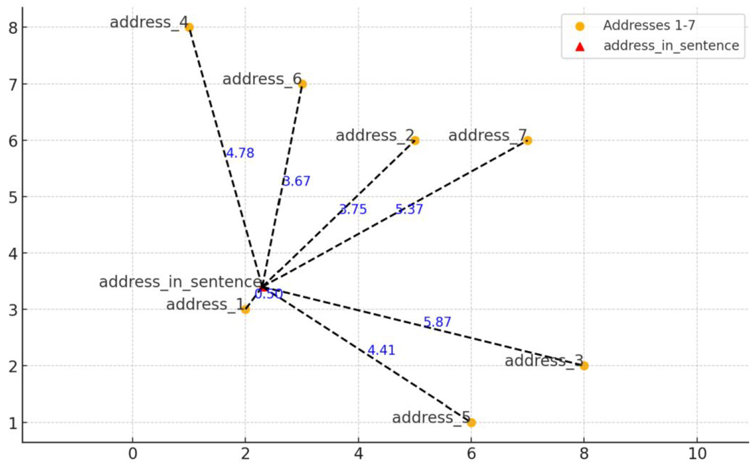
A simplified diagram of semantic annotation.

The fourth step involved counting the frequency of each sense and computing the percentage. Once all instances of a word in the BNC were semantically annotated, different senses of the same word were treated as different items. As a result, we could count senses and calculate their frequency as effortlessly as we count words in conventional methods.

Accuracy Check

After semantic annotation, we evaluated annotation accuracy. In previous studies, accuracy is commonly assessed through inter-rater consensus. The annotated texts are submitted to two experts, who will determine whether the result is correct or not. The extent to which the two experts are in agreement with each other will be reported. It is impossible to adopt similar manual methods because about 70 million instances of 11,000 senses are annotated and thus need to be checked in this study.

We adopted the train-test split technique, a machine learning practice where data is divided into two subsets: a training set (70% of OED examples) to teach BERT how to map senses to vectors, and a test set (30%) to evaluate its performance on unseen data. The example sentences from the OED are divided into two groups: a training group and a test group. The test group, which represents 30% of the example sentences, was mixed with sentences from the BNC to undergo unbiased annotation by BERT. After annotation, the example sentences were extracted and their annotations were compared with their original definitions. The accuracy rate for each word was then computed and reported.

High-Frequency Sense Selection

A large number of English words have multiple meanings. A high-frequency word list offering semantic description can be of greater help. In response to Szudarski’s (2017) doubt about what beginning learners should start with when consulting a word list, we identified high-frequency senses for each GSL word.

Following the selection criteria for creating GSL, the selection of high-frequency senses followed a structured four-phase process to ensure methodological transparency and pedagogical relevance.

First, a quantitative thresholding approach was applied: senses of each word were ranked in descending order of frequency, and their percentages were cumulatively summed until reaching 90% of the word’s total occurrences. This threshold, informed by prior pedagogical lexicography studies (D. Gardner & Davies, 2014; Garnier & Schmitt, 2015), balances coverage breadth with list conciseness.

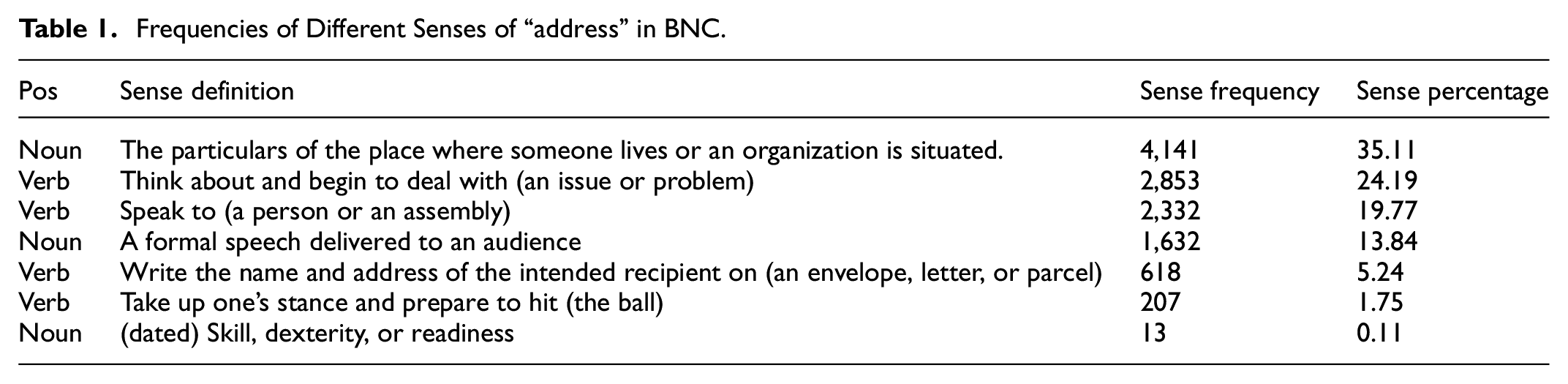
In this adding-up process, only senses exceeding 10% would be calculated. To illustrate this process, let’s consider the example of the word “address” in the BNC corpus. Table 1 presents the frequency and percentage of its different senses. The most prevalent sense is the “place” sense, which appears 4,141 times in the BNC and accounts for 35.11% of its total occurrences. It is followed by the senses of “dealing with a problem,” “speaking to,” and “a formal speech.” The percentage of each sense was added up cumulatively until it reached 90% (35.11% + 24.19% + 19.77% + 13.84% = 92.91%). Consequently, only the first four senses were identified as high-frequency senses.

Table 1.

Frequencies of Different Senses of “address” in BNC.

Pos	Sense definition	Sense frequency	Sense percentage
Noun	The particulars of the place where someone lives or an organization is situated.	4,141	35.11
Verb	Think about and begin to deal with (an issue or problem)	2,853	24.19
Verb	Speak to (a person or an assembly)	2,332	19.77
Noun	A formal speech delivered to an audience	1,632	13.84
Verb	Write the name and address of the intended recipient on (an envelope, letter, or parcel)	618	5.24
Verb	Take up one’s stance and prepare to hit (the ball)	207	1.75
Noun	(dated) Skill, dexterity, or readiness	13	0.11

Second, a minimum individual contribution criterion was enforced: only senses constituting at least 10% of a word’s frequency were eligible for inclusion. This excluded marginal senses (e.g., “address-skill” at 0.11%) that add minimal pedagogical value.

Exceptions occurred when cumulative coverage remained below 90% even after including all eligible senses (e.g., “around” retained three senses totaling 54.1%). This can be illustrated by the word “around” in Table 2. Of the 10 senses listed, only three have a percentage higher than 10%. In such cases, only these three senses are considered as high-frequency senses.

Table 2.

High-frequency Senses of “Around.”

Pos	Sense definition	Sense frequency	Sense percentage
Preposition	On every side of	11,549	26.63
Adverb	(used with a number or quantity) approximately	7,257	16.73
Adverb	Present, living, in the vicinity, or in active use	4,660	10.74

Third, qualitative filtering removed senses labeled in OED as archaic, dialectal, derogatory, or domain-specific (e.g., “city = London financial district”), adhering to West’s (1953) principle of stylistic neutrality but replacing subjective judgment with dictionary-based objectivity.

There is always debate about whether frequency alone is adequate to produce a satisfactory word list. In addition to frequency, several other factors, including difficulty of learning, necessity, coverage, stylistic level, and emotional neutrality were considered during the creation of GSL (West, 1953: x). Brezina and Gablasova (2015) argued that the inclusion of such subjective measures made the result hard to check and reproduce.

In response to both arguments, we incorporate some subjective considerations, such as register (“formal” or “informal”). However, unlike previous studies, we did not rely on human judgment. Rather, we used labels provided in the OED as a criterion. To be specific, any senses labeled in OED as “formal,” “literary,” “informal,” “archaic,” “dated,” “vulgar slang,” “rare,” “dialect,” or “derogatory” were excluded from our high-frequency sense list (see Table 3). In this way, although we used some qualitative standards as West (1953) did, the whole process can still be easily replicated and the result can be easily verified or updated.

Removing such stylistically marked senses, in some cases, leads to the entire disappearance of certain GSL words. For example, all senses of the word “thus” in OED are classified as “formal” and “literary” (see Table 4). Consequently, the word “thus” in GSL is excluded from our final list of high-frequency senses.

Table 4.

Senses of “Thus” in the OED.

Lemma	Pos	Register	Sense definition
Thus	Adverb	Formal, literary	As a result or consequence of this; therefore.
Thus	Adverb	Formal, literary	In the manner now being indicated or exemplified; in this way.
Thus	Adverb	Formal, literary	To this point; so.

When creating GSL, West (1953) adopted stylistic and emotional neutrality as a criterion in addition to frequency. He removed such words as “personage,” “fellow” and “chap” because “personage is the written and rather literary equivalent of person,” and “fellow or chap is the colloquial equivalent” (West, 1953: x). He argued that the foreign learner did not at this stage need either high or low equivalent in his conversation but should keep a middle path.

However, each sense of “thus” is labeled as “formal” in the OED nowadays. It does not necessarily mean that West did not adhere to his criterion of stylistic neutrality. The perception of what is considered formal may have changed over time. What may have been deemed formal in contemporary times was not considered as such in West’s era.

Fourth, the draft list was submitted to two professors who specialized in foreign language education for a thorough assessment. They reached a consensus that senses primarily used in specific academic fields or technical areas were not necessary for beginning learners and had better be eliminated. For each sense included, we closely read the corresponding definition in the OED and eliminate senses labeled with an academic discipline or primarily used in specific fields. A few examples can be found in Table 5.

Table 5.

Examples of Technical Senses.

Lemma	Sense definition
Idea	Philosophy (in Platonic thought) an eternally existing pattern of which individual things in any class are imperfect copies.
Elastic	Economics (of demand or supply) sensitive to changes in price or income.
City	= the City of London

Verification

To verify the validity of this list, we calculated the coverage of the high-frequency senses and then compared it with the coverage of all GSL headwords in different corpora. The term “coverage” refers to the percentage of words in a corpus covered by items from a particular word list. It is used as the most important criterion in previous studies evaluating high-frequency word lists (Brezina & Gablasova, 2015; Dang et al., 2022; Dang & Webb, 2016). We hypothesize that though high-frequency senses make up a small percentage of the GSL list, they can achieve a significant coverage comparable to the entire list.

It is not adequate to check the coverage of a word list only in the corpus which it is derived from. Therefore, we further assessed the coverage of both GSL words and high-frequency senses in another two English Corpora, namely LOB and CLOB.

Result and Discussion

After semantic annotation using BERT, each word in the BNC was tagged with a “sense label” in addition to its original labels, which include “source_file,” “text_type,” “sent_num,” “word,” “lemma,” “pos,” and “C5.” This update is illustrated in Figure 4, where the last column represents the newly added sense label. For example, “mono” means that the word has only one meaning in the OED, while “0” means that the first sense of the word in the OED is selected as the correct meaning. With a semantically annotated corpus, we can treat each word associated with a specific sense as a distinct item. This allows us to count the various senses and identify those that occur frequently.

Figure 4.

A snapshot of the BNC after semantic annotation.

Semantic Frequency of GSL Words and Annotation Accuracy (Addressing RQ1)

The study produced a comprehensive list of senses for GSL words. This might be the first time to re-calculate the semantic frequencies of GSL words after they were originally calculated in 1953. Our list is consciously structured to resemble the original arrangement of GSL. Words are organized alphabetically, accompanied by detailed data for each sense. To be specific, each sense entry includes information on “lemma,” “pos”, “sense definition,” “example,” “sub-sense definition,” “lemma frequency,” “semantic frequency,” “percentage,” “accuracy,” etc.

The information on “sense definition,” “sub-sense definition,” “example,” and “register” have all been sourced from the OED. To ensure greater accuracy, we used the general-level senses when annotating corpora. Nevertheless, we also provide sub-senses for readers’ reference. “Lemma frequency” refers to the overall frequency of a word in the BNC. “Semantic frequency,” the most important information in this article, indicates the number of occurrences that specifically correspond to a particular sense, and “percentage” represents the proportion of each sense in relation to the total number of instances. “Accuracy” refers to the percentage of how many testing sentences are correctly annotated.

Table 6 presents some key data on the semantic frequency of the word “act.” Within the BNC corpus, “act” appears 38,425 times. Of these occurrences, 17,686 instances are associated with the meaning of “a written law,” making up 46.03% of the total. The second most common meaning is “taking action,” which occurs 5,073 times, representing 13.2%. The least frequent sense (excluding phrasal verbs) is that of “pretense,” present in only 439 instances, accounting for a mere 1.14%. The three senses can be illustrated with the following examples respectively.

(1) the 1989 Children Act

(2) They urged Washington to act.

(3) She was putting on an act and laughing a lot.

Table 6.

Semantic Frequency of “Act.”

Lemma	Pos	Sense definition	Sub senses	Sense frequency	Lemma frequency	Percentage (%)
Act	Verb	Take action; do something.		5,073	38,425	13.2
Act	Verb	Behave in the way specified.		1,843	38,425	4.8
Act	Verb	Take effect; have a particular effect.		4,332	38,425	11.27
Act	Verb	Perform a role in a play, film, or television.	1. Behave so as to appear to be; pretend to be.	2,248	38,425	5.85
Act	Noun	A thing done; a deed.	1. A New Testament book immediately following the Gospels and relating the history of the early Church.	4,696	38,425	12.22
Act	Noun	A pretense.	1. A particular type of behavior or routine.	439	38,425	1.14
Act	Noun	A written law passed by Parliament, Congress, etc.	1. A document attesting a legal transaction.	17,686	38,425	46.03
Act	Noun	A written law passed by Parliament, Congress, etc.	2. The recorded decisions or proceedings of a committee or an academic body.	17,686	38,425	46.03
Act	Noun	A main division of a play, ballet, or opera.	1. A set performance.	1,771	38,425	4.61
Act	Noun	A main division of a play, ballet, or opera.	2. A performing group.	1,771	38,425	4.61
Act on	Phrasal verb			68	38,425	0.18
Act up	Phrasal verb			25	38,425	0.07
Act out	Phrasal verb			244	38,425	0.64

Phrasal verbs are counted separately in this study. Unlike previous studies where words within phrasal verbs were matched with a standard sense entry in the dictionary, we address a phrasal verb as a whole unit. For instance, the meaning of “act” in “act on” was traditionally interpreted based on one of the first eight senses in Table 6. We, however, list them separately alongside the standard sense entries. While acknowledging that phrasal verbs can have multiple meanings, we treated each phrasal verb listed in the OED as a distinct entry without delving into its various sub-senses. We make such a compromise because we find, after several experiments, that BERT cannot accurately disambiguate the meanings of phrasal verbs compared to single words.

After annotating all the GSL words in BNC, we get a comprehensive list of about 11,000 senses. This list is carefully reviewed. It is found that 10 words, such as “farmer,” “victory,” “village,” and “wife,” have two entries in the OED. One is uncommon and has no example sentences. For example, one homonym of “victory” is defined as “The flagship of Lord Nelson at the Battle of Trafalgar, launched in 1765.” BERT relies on example sentences to extract vectors. In the absence of example sentences, BERT is unable to perform any analysis on these words. These 10 senses are rather uncommon and are therefore deleted, and the percentage of the remaining sense is designated as “≈100”. The final list now includes 1,875 words with 10,925 senses.

BERT demonstrates 92% accuracy when annotating the GSL words. This accuracy result is similar to previous studies (Hu et al., 2019; L. Liu et al., 2024), and is higher than those of previous sense disambiguation studies (Kilgarriff, 2001; Snyder & Palmer, 2004).

As specified in Section 3.2, 30% of the example sentences from the definition of the GSL words in the OED are mixed in the BNC for BERT to annotate indiscriminately. There are a total of 1,875 headwords in GSL and the test set contains 80,330 example sentences. On average, 43 example sentences are used to check the annotation accuracy of one word. When compared with the original definition in OED, 73,781 sentences are found to be correctly annotated, resulting in an overall accuracy of 92%.

Descriptive statistics of annotation accuracy can be found in Table 7. The minimum is 0.63, the maximum is 1, and the mean is 0.94.

Table 7.

Descriptive Statistics of Accuracy.

Variable	n	Mean	sd	Median	Min	Max
Accuracy	1,859	0.94	0.06	0.95	0.63	1.00

The histogram of annotation accuracy is shown in Figure 5. It can be observed that approximately 75.26% (24.1 + 51.16) of the words have a classification accuracy of 90% or higher. Approximately 97.48% (6.46 + 15.76 + 24.1 + 51.16) of the words have a classification accuracy of 80% or higher.

Figure 5.

Histogram of accuracy.

This shows that BERT can annotate large corpora automatically and count sense frequency with high precision.

Selection of High-Frequency Senses (Addressing RQ2)

A list of 3,695 senses are identified as high-frequency senses after applying the criteria specified in Section 3.2.

We deliberately make a long list. We set the cut-off line at 90%, while Garnier and Schmitt’s (2015) cut-off point for creating a phrase list is at 75%. There is no universally agreed threshold value in studies of high-frequency vocabulary. Different researchers typically select their value after extensive experimentation. Garnier and Schmitt (2015) opted for a threshold of 75%, stating that this decision was made after careful examination of the data yielded by the corpus search. D. Gardner and Davies (2014) stated this clearly when discussing their threshold values. They pointed out that “there is nothing particularly special about the 1.5 Ratio, as there is no commonly accepted value for this measure” (D. Gardner & Davies, 2014: 315). As we settle upon the threshold of 90%, our list may potentially include a greater number of senses than strictly required for beginning learners. The rationale behind constructing a long list lies in its flexibility for future modification: it is much easier to delete what you think is unnecessary from a long list than to add what you think is necessary to a short list. The complete list of high-frequency senses of GSL words is attached as an appendix to this article.

After reviewing the list, we want to highlight three important features of these high-frequency senses of GSL words.

First, a limited number of senses account for a large proportion of a word’s meaning. While many English words have many senses, they usually have only a limited number of high-frequency senses. Specifically, for approximately 50% of the GSL words, a single sense encompasses no less than 70% of their overall meaning. For example, the word “about” has six senses in the OED. The sense of “on the subject of; concerning” alone takes up 73.14%, while four other senses collectively amount to less than 10%. Similar examples can be found in Table 8.

Table 8.

Examples of High-Frequency Senses.

Lemma	Sense	Sub-sense	Percentage (%)
Able	Having the power, skill, means, or opportunity to do something.		96.26
Abroad	In or to a foreign country or countries.		65.72
Admit	Confess to be true or to be the case.	1. Confess to (a crime or fault, or one’s responsibility for it)	78.63
Admit	Confess to be true or to be the case.	2. Acknowledge (a failure or fault)	78.63
Age	The length of time that a person has lived or a thing has existed.	1. A particular stage in someone’s life.	64.58
Age		2. The state of being old.	64.58

Among the 11,000 senses of GSL headwords, approximately one-third of the senses cover about 90% of all occurrences. It has been repeatedly pointed out that high-frequency words take up a large portion of corpora while words of lower frequency provide a progressively smaller coverage. The distribution of semantic frequency is similar to that of word frequency: high-frequency senses hold a considerable proportion.

Second, many figurative or extended meanings are frequently used. Take, for instance, the verb “aim,” which has two senses (see Table 9). The extended interpretation of “having the intention of achieving” occurs frequently in the BNC.

Table 9.

Semantic Frequency of “Aim.”

Lemma	Pos	Sense	Percentage (%)
Aim	Noun	A purpose or intention; a desired outcome.	44.8
Aim	Verb	Have the intention of achieving.	32.4
Aim	Verb	Point or direct (a weapon or camera) at a target.	18.05

Likewise, as shown in Table 10, the “defeat” meaning of “beat” occurs almost three times more frequently than the “strike” meaning, while the meaning of “be important to” in “key” is significantly more common than its literal “instrument” meaning. Examples of different meanings of “beat” and “key” can be found in sentences 4 to 7 below. These metaphorical meanings of some common words are often neglected in existing middle school teaching guideline documents.

(4) She beat him easily at chess.

(5) A man was found beaten to death.

(6) She became a key figure in the suffragette movement.

(7) There were two keys to the cupboard.

Table 10.

Comparison of Metaphorical and Literal Senses.

Lemma	Pos	Sense	Percentage (%)
Beat	Verb	Defeat (someone) in a game or other competitive situation.	46.56
Beat	Verb	Strike (a person or an animal) repeatedly and violently so as to hurt or injure them, typically with an implement such as a club or whip.	15.99
Key	Adjective	Of crucial importance.	51.49
Key	Noun	A small piece of shaped metal with incisions cut to fit the wards of a particular lock, which is inserted into a lock and turned to open or close it.	14.83

Third, a large number of high-frequency senses stay generally stable through time. Many frequent senses in the GSL remain highly frequent in the BNC. The GSL is frequently criticized for being out of date. However, Brezina and Gablasova (2015) found that a majority of the first 1,000 words in their New-GSL are also included in GSL. It means that a large part of high-frequency words remain stable. Similarly, we find that many high-frequency senses in the GSL remain frequent in the BNC. Some senses such as the “foreign country” sense of “abroad” or the “disaster” sense of “accident” can be confidently claimed according to common sense. On the other hand, some senses, such as that of “apply” and “argue” in Table 11, might not have been asserted without support from the investigation.

Table 11.

Examples of Stable High-Frequency Senses.

Lemma	Sense	GSL (%)	BNC (%)
Abroad	In or to a foreign country or countries.	80	65.72
Accident	An unfortunate incident that happens unexpectedly and unintentionally, typically resulting in damage or injury.	72	71.09
Apply	Be applicable or relevant.	52	60.28
Argue	Give reasons or cite evidence in support of an idea, action, or theory.	57	89.26

Moreover, even some percentage figures remain relatively stable. For instance, the percentage of the two senses of “familiar” is similar between the GSL and the BNC (see Table 12).

Table 12.

Constant Sense Percentages.

Lemma	Sense	GSL (%)	BNC (%)
False	Not according with truth or fact	40	51.31
False	Made to imitate something in order to deceive.	20	28.77
Familiar	Well known from long or close association.	60	62.58
Familiar	In close friendship; intimate.	38	36.52

On the other hand, we also find that certain meanings of words vary in frequency over time. Such changes, similar to word frequency changes, are usually a result of societal changes. For example, it is found that the senses that are associated with computer science are increasing. Some computer-related senses which are not even included in the GSL began to account for more than 10% of the BNC. Some senses related to religion or political life became less frequent. The “parliament” sense of “bill” and the “principal site” sense of “seat” have diminished over time. Some other declined senses were once associated with formal style. These senses are now labeled as “old use or formal” in modern dictionaries and are less commonly used. For example, the “except” meaning of “save” occupies a significant portion (14%) in the GSL, yet it is nearly negligible (0.02%) in the BNC.

At the beginning of our study, we planned to compare our semantic frequency data with that of the GSL on a sense-by-sense basis. The aim was to determine which senses remain stable and how large a percentage they account for. However, we quickly found that a direct comparison was not possible due to the different sense entries used in the two studies. West relied on Lorge and Thorndike’s semantic frequency count, which drew its sense entries from the OED (1933). For potential comparison, we purposefully opt to use the OED as well. Nevertheless, West took it upon himself to “group the meanings more coarsely” to make the information more accessible to users (West, 1953: vii). For example, the 22 senses of the word “game” in the OED were lumped into 4 senses in the GSL. West did not specify the methodology or principles behind his sense grouping. Whatever it might be, it was not applied systemically. Some regular polysemy words like “bottle” or “cup” can express both “container ” or “quantity.” Such regular polysemy can be categorized as a single sense as in Cambridge Learners’ Dictionary or as two different senses as in Oxford Learners’ Dictionary. However, in the GSL, “bottle” has two senses while “cup,” “bowl,” and “box” each contain only one sense. It is therefore impossible to apply West’s sense grouping rule. This constitutes the major obstacle to a systematic comparison.

As a result of the difference in sense entries used in the two studies, we read both lists in person and identified which senses are most stable and which senses are most different. While we can not provide exact numbers, we find a significant number of high-frequency meanings of commonly used English words remain relatively stable.

Verification of Selected Senses (Addressing RQ3)

In various corpora, the high-frequency senses make up approximately 60% of the total coverage. This percentage is significant when compared to the coverage of all the senses of GSL headwords.

The GSL headwords, in total, have 10,925 senses, of which 3,695 are high-frequency senses, taking up about one-third of all the senses. When considering the coverage in the BNC, all these senses together cover 71.83%, whereas the high-frequency senses alone cover 62.14%. This means that by removing two-thirds of the senses, we only lose 10% of the overall coverage.

As also shown in Table 13, the coverage of these high-frequency senses is stable in different corpora. It is 62.14% in the BNC, 59.78% in LOB, and 58.15% in CLOB respectively. Even though these corpora represent various periods in the development of the English language, the coverage of high-frequency senses remains relatively constant at approximately 60%. The coverage in the BNC is a bit higher. This may be because the BNC is the corpus where these high-frequency senses are derived. The percentage is high when compared with the coverage of all the senses. The coverage of all the senses of the 1,875 headwords is approximately 71.87% in LOB, 71.83% in the BNC, and 71% in CLOB respectively.

Table 13.

Coverage of High-frequency Senses and All Senses in the BNC, LOB, and CLOB.

Corpus	Coverage of high-frequency senses (%)	Coverage of all senses (%)
Number of senses	3,695	10,925
BNC	62.14	71.83
LOB	59.78	71.87
CLOB	58.15	71

To sum up, these high-frequency senses achieve significant coverage with far fewer items, and they achieve consistent coverage across different corpora

Theoretical Implication

In this study, we use a BERT model to represent words with vectors and compute the frequency of senses. It shows a pioneering way to annotate large corpora with semantic information and compute semantic frequency.

It addressed the long-standing need to investigate semantic frequency in large corpora. D. Gardner (2007) pointed out that corpus research based on the frequency of word forms, without consideration of word meanings, will invariably result in problems. D. E. E. Gardner and Davies (2007) similarly argued for ranking the semantic frequency of phrasal verbs, thus prioritizing high-frequency senses for language learning. They advocated a counting unit that combines a single form with a single sense, rather than considering words with multiple unrelated meanings as a single entity. Such proposals have never been implemented due to technical constraints. To treat different senses individually, we have to construct semantically annotated corpora first. Until the development of recent large language models like BERT, this mission has been “much easier talked about than done” (D. E. E. Gardner & Davies, 2007: 353).

This study shows a pioneering way to semantically annotate large corpora. Once a corpus is annotated, each sense can be treated as a distinct item. Consequently, we can count senses in large corpora and identify high-frequency senses. To illustrate the annotation process, we calculate the sense frequency of the GSL words in the BNC. Some may express concerns that the BNC does not accurately represent contemporary language features, given that it was created in the 1990s. We choose to use the BNC because the full text of more recent corpora, such as the “BNC 2014”, is not yet accessible, which makes the BNC the second-best choice. This compromise does not diminish the pedagogical value of our list; in fact, the consistent coverage of high-frequency senses across different corpora indicates that they remain relatively stable over time.

Two advantages of this method can be highlighted. First, it can be easily applied to studies examining the sense frequency of other word lists. None of the large corpora, such as the COCA or the BNC, has been semantically annotated. None of the existing word lists like Nation’s (2012) BNC/COCA List, Browne et al. (2013) NGSL, or Brezina and Gablasova’s (2015) New-GSL provides semantic frequency data. When the full texts of these corpora are available, the method outlined in this study can be readily applied. Second, the process is easily replicable, which facilitates the verification of results. West’s GSL has faced criticism because its findings can be hard to expand or update due to the underlying methodology. Previous studies (Brezina & Gablasova, 2015; Gilner & Morales, 2008) have pointed out that the combination of quantitative and qualitative criteria used in creating the GSL complicates updates. We also highlighted above that West grouped the sense entries in the OED without consistent principles. In contrast, the method from this study is clear and straightforward, allowing for step-by-step replication and making it easy to verify or update results.

In addition to identifying high-frequency senses, this method can help to solve many theoretical issues. First, we can track semantic changes in a large sample of words over a long period. Previous studies of semantic change usually relied on manual counting, and have therefore focused on only a limited number of words. A semantically annotated corpus allows us to describe semantic changes in a large sample of words. We are now annotating the Corpus of Historical American English (COHA) and calculating the sense frequency of words in different periods, aiming to find out those true stable words, words that remain stable in both form and meaning during a long period. Second, we can solve the controversy of whether a common word such as “paper” is an academic word or not. Previous research presented two contrasting viewpoints on this issue. Some studies argue that academic word lists should exclude common words because learners at the beginner level often encounter these words in daily life and may have already mastered them. On the other hand, some other studies argue that academic word lists should include such common words because these words often carry specific “academic meanings” in scholarly texts that differ significantly from their everyday usage. Once different senses of common words are distinguished and counted as different items, this controversy will be solved.

Conclusion

High-frequency word lists have been created to help foreign language learners identify which words to prioritize for their studies. However, most of these lists do not specify which meanings are most important.

We use a BERT model to calculate the frequencies of different senses for words from the GSL. We analyzed the sense frequency of the GSL words and identified a total of 3,695 high-frequency senses. It is found that BERT can annotate senses accurately, achieving a 92% accuracy when annotating the GSL words, and the high-frequency senses we identified achieve stable coverage in several corpora. What’s more, no manual intervention is involved in semantic annotation and sense calculation. Therefore, this method can be easily applied in future studies.

While we acknowledge that both the GSL and the BNC are not modern resources, we still believe that identifying high-frequency senses enhances the pedagogical value of the GSL. First, the BNC is the most recent corpus of which full texts can be downloaded today. More recent corpora are not available for semantic annotation. Second, high-frequency senses tend to remain generally stable, as demonstrated by their consistent coverage across various corpora and our manual comparisons with the original GSL.

The field of large language models has seen notable advancements, particularly since the year 2022. Along with these technical advances, semantic frequency studies will be resumed and carried out at a faster pace and with higher accuracy.

Supplemental Material

sj-xlsx-1-sgo-10.1177_21582440251333182 – Supplemental material for Calculating Semantic Frequency of GSL Words Using a BERT Model in Large Corpora

Supplemental material, sj-xlsx-1-sgo-10.1177_21582440251333182 for Calculating Semantic Frequency of GSL Words Using a BERT Model in Large Corpora by Liu Lei, Gong Tongxi, Shi Jianjun and Guo Yi in SAGE Open

Footnotes

Acknowledgements

Thank you to the anonymous reviewers for their insightful comments, which have greatly improved the quality of the manuscript.

ORCID iDs

Liu Lei

Gong Tongxi

Ethics Approval and Informed Consent Statements

This article does not contain any studies with human or animal participants.

Author Contributions

LL: Data curation, Writing – original draft & review. GT: Writing – original draft. SJ: Conceptualization, Writing – review & editing. GY: Validation, Writing – review & editing.

Funding

The author(s) disclosed receipt of the following financial support for the research, authorship, and/or publication of this article: This work was supported by Shanghai Philosophy and Social Science Planning Fund Project [grant number 2021ZYY003], National Social Science Fund of China [grant number 22AYY024], Ministry of Education Industry-University Collaborative Education Program [grant number 241001713140345], and Henan Province Philosophy and Social Science Project [grant number 2024BYY014], Postgraduate Education Reform and Quality Improvement Project of Henan Province [YJS2025AL15].

Declaration of Conflicting Interests

The author(s) declared no potential conflicts of interest with respect to the research, authorship, and/or publication of this article.

Data Availability

The datasets presented in this article are not readily available because they can be used for academic purpose only. Requests to access the datasets should be directed to the corresponding author.

Supplemental Material

Supplemental material for this article is available online.

References

Agirre

Soroa

(2009, March). Personalizing pagerank for word sense disambiguation [Conference session]. Proceedings of the 12th Conference of the European Chapter of the ACL (EACL 2009). https://doi.org/10.3115/1609067.1609070

Beck

(2020). DiaSense at SemEval-2020 task 1: Modeling sense change via pre-trained BERT embeddings [Conference session]. Proceedings of the Fourteenth Workshop on Semantic Evaluation.

Brezina

Gablasova

(2015). Is there a core general vocabulary? Introducing the new general service list. Applied Linguistics, 36(1), 1–22. https://doi.org/10.1093/applin/amt018

Browne

Culligan

Phillips

(2013). The new general service list. http://www.newgeneralservicelist.org

Coxhead

(2000). A new academic word list. TESOL Quarterly, 34(2), 213–238. https://doi.org/10.2307/3587951

Dang

T. N. Y.

Webb

(2016). Evaluating lists of high-frequency words. ITL - International Journal of Applied Linguistics, 167(2), 132–158. https://doi.org/10.1075/itl.167.2.02dan

Dang

T. N. Y.

Webb

Coxhead

(2022). Evaluating lists of high-frequency words: Teachers’ and learners’ perspectives. Language Teaching Research, 26(4), 617–641. https://doi.org/10.1177/136216882091118

Davies

Gardner

(2010). A frequency dictionary of contemporary American English. Routledge.

Devlin

Chang

M. W.

Lee

Toutanova

(2018). Bert: Pre-training of deep bidirectional transformers for language understanding. arXiv preprint arXiv:1810.04805.

10.

Sun

(2019). Using BERT for word sense disambiguation. arXiv preprint arXiv:1909.08358.

11.

Ettinger

(2020). What BERT is not: Lessons from a new suite of psycholinguistic diagnostics for language models. Transactions of the Association for Computational Linguistics, 8(1), 34–48. https://doi.org/10.1162/tacl_a_00298

12.

Gardner

(2007). Validating the construct of word in applied corpus-based vocabulary research: A critical survey. Applied Linguistics, 28(2), 241–265. https://doi.org/10.1093/applin/amm010

13.

Gardner

Davies

(2014). A new academic vocabulary list. Applied Linguistics, 35(3), 305–327.

14.

Gardner

Davies

(2007). Pointing out frequent phrasal verbs: A corpus-based analysis. TESOL Quarterly, 41(2), 339–359. http://www.jstor.org/stable/40264356

15.

Garnier

Schmitt

(2015). The PHaVE list: A pedagogical list of phrasal verbs and their most frequent meaning senses. Language Teaching Research, 19(6), 645–666. https://doi.org/10.1177/13621688145597

16.

Gilner

Morales

(2008). Corpus-based frequency profiling: Migration to a word list based on the British National Corpus. The Buckingham Journal of Language and Linguistics, 1, 41–57. https://doi.org/10.5750/bjll.v1i0.3

17.

Goldberg

(2019). Assessing BERT’s syntactic abilities. arXiv preprint arXiv:1901.05287.

18.

Huang

Sun

Qiu

Huang

(2019). GlossBERT: BERT for word sense disambiguation with gloss knowledge [Conference session]. Proceedings of the 2019 Conference on Empirical Methods in Natural Language Processing and the 9th International Joint Conference on Natural Language Processing (EMNLP-IJCNLP).

19.

Liang

(2019). Diachronic sense modeling with deep contextualized word embeddings: An ecological view [Conference session]. Proceedings of the 57th Annual Meeting of the Association for Computational Linguistics. https://doi.org/10.18653/v1/P19-1379

20.

Iacobacci

I. J.

Pilehvar

M. T.

Navigli

(2016). Embeddings for word sense disambiguation: An evaluation study [Conference session]. 54th Annual Meeting of the Association for Computational Linguistics, ACL 2016-Long Papers.

21.

Kilgarriff

(2001, July). English lexical sample task description [Conference session]. Proceedings of SENSEVAL-2 Second International Workshop on Evaluating Word Sense Disambiguation Systems. https://doi.org/10.5555/2387364.2387368

22.

Lin

Wang

(2019). A corpus-driven study of semantic changes of English adverb AGAIN: A diachronic perspective. Foreign Languages and Their Teaching, 2(34), 73–83.

23.

Liu

C. Y.

(2023). A corpus-based study of vocabulary in massive open online courses (MOOCs). English for Specific Purposes, 72(1), 40–50.

24.

Liu

Gong

Shi

Guo

(2024). A high-frequency sense list. Frontiers in Psychology, 15, 1430060.

25.

Liu

N. F.

Gardner

Belinkov

Peters

M. E.

Smith

N. A.

(2019). Linguistic knowledge and transferability of contextual representations. arXiv preprint arXiv:1903.08855.

26.

Loureiro

Rezaee

Pilehvar

M. T.

Camacho-Collados

(2021). Analysis and evaluation of language models for word sense disambiguation. Computational Linguistics, 47(2), 1–443.

27.

Luo

Liu

Xia

Sui

Chang

(2018). Leveraging gloss knowledge in neural word sense disambiguation by hierarchical co-attention [Conference session]. Proceedings of the 2018 Conference on Empirical Methods in Natural Language Processing.

28.

Melamud

Goldberger

Dagan

(2016, August). context2vec: Learning generic context embedding with bidirectional lstm [Conference session]. Proceedings of the 20th SIGNLL Conference on Computational Natural Language Learning.

29.

Miller

G. A.

(1995). WordNet: A lexical database for English. Communications of the ACM, 38(11), 39–41. https://doi.org/10.1145/219717.219748

30.

Moro

Raganato

Navigli

(2014). Entity linking meets word sense disambiguation: A unified approach. Transactions of the Association for Computational Linguistics, 2, 231–244.

31.

Nation

I. S. P.

(2001). Learning vocabulary in another language (Vol. 10). Cambridge University Press.

32.

Nation

I. S. P.

(2012). The BNC/COCA word family list. https://www.wgtn.ac.nz/lals/resources/paul-nations-resources/paul-nations-publications/publications/documents/Information-on-the-BNC_COCA-word-family-lists.pdf

33.

Nation

I. S. P.

(2016). Making and using word lists for language learning and testing. John Benjamins Publishing.

34.

Nation

I. S. P.

Waring

(1997). Vocabulary size, text coverage, and word lists. In Schmitt

Michael

(Eds.), Vocabulary: Description, acquisition and pedagogy (pp. 6–19). Cambridge University Press.

35.

Pawar

Thombre

Mittal

Ponkiya

Bhattacharyya

(2021). Tapping BERT for preposition sense disambiguation. arXiv preprint arXiv:2111.13972.

36.

Peters

Neumann

Iyyer

Gardner

Clark

Lee

Zettlemoyer

(2018). Deep contextualized word representations [Conference session]. Proceedings of the 2018 Conference of the North American Chapter of the Association for Computational Linguistics: Human Language Technologies, Volume 1 (Long Papers). https://doi.org/10.18653/v1/N18-1202

37.

Radford

Narasimhan

Salimans

Sutskever

(2018). Improving language understanding by generative pre-training. https://cdn.openai.com/research-covers/language-unsupervised/language_understanding_paper.pdf

38.

Raganato

Bovi

C. D.

Navigli

(2017a, September). Neural sequence learning models for word sense disambiguation [Conference session]. Proceedings of the 2017 Conference on Empirical Methods in Natural Language Processing.

39.

Raganato

Camacho-Collados

Navigli

(2017b). Word sense disambiguation: a uinified evaluation framework and empirical comparison [Conference session]. Proceedings of the 15th Conference of the European Chapter of the Association for Computational Linguistics: Volume 1, Long Papers.

40.

Richards

J. C.

(1974). Word lists: Problems and prospects. RELC Journal, 5(2), 69–84. https://doi.org/10.1177/0033688274005002

41.

Schlechtweg

McGillivray

Hengchen

Dubossarsky

Tahmasebi

(2020). SemEval-2020 task 1: Unsupervised lexical semantic change detection. arXiv preprint arXiv:2007.11464.

42.

Schmitt

(2010). Researching vocabulary: A vocabulary research manual. Springer.

43.

Schmitt

Dunn

O’Sullivan

Anthony

Kremmel

(2021). Introducing knowledge-based vocabulary lists (KVL). TESOL Journal, 12(4), 1–10. https://doi.org/10.1002/tesj.622

44.

Schmitt

(2020). Vocabulary in language teaching. Cambridge University Press.

45.

Snyder

Palmer

(2004, July). The English all-words task [Conference session]. Proceedings of SENSEVAL-3, the Third International Workshop on the Evaluation of Systems for the Semantic Analysis of Text. https://aclanthology.org/W04-08

46.

Szudarski

(2017). Corpus linguistics for vocabulary: A guide for research. Routledge.

47.

Tenney

Xia

Chen

Wang

Poliak

McCoy

R. T.

Pavlick

(2019). What do you learn from context? Probing for sentence structure in contextualized word representations. arXiv preprint arXiv:1905.06316.

48.

Vaswani

Shazeer

Parmar

Uszkoreit

Jones

Gomez

A. N.

Polosukhin

(2017). Attention is all you need [Conference session]. Proceedings of the 31st International Conference on Neural Information Processing Systems. https://doi.org/10.48550/arXiv.1706.03762

49.

Vilkaitė-Lozdienė

Schmitt

(2020). Frequency as a guide for vocabulary usefulness: Hi-, mid-, and low-frequency words. In Webb

(Ed.), The Routledge handbook of vocabulary studies (pp. 81–96). Routledge.

50.

Vuković-Stamatović

(2022). Suitability of science & technology documentaries for EAP and EST listening. Journal of English for Academic Purposes, 58, 101137.

51.

Wang

(2020, November). A synset relation-enhanced framework with a try-again mechanism for word sense disambiguation [Conference session]. Proceedings of the 2020 Conference on Empirical Methods in Natural Language Processing (EMNLP).

52.

West

(1953). A general service list of English words: With semantic frequencies and a supplementary word-list for the writing of popular science and technology. Longman.

53.

Wiedemann

Remus

Chawla

Biemann

(2019). Does BERT make any sense? Interpretable word sense disambiguation with contextualized embeddings. arXiv preprint arXiv:1909.10430.

54.

Schuster

Chen

Q. V.

Norouzi

Macherey

Dean

(2016). Google’s neural machine translation system: Bridging the gap between human and machine translation. arXiv preprint arXiv:1609.08144.

55.

Yuan

Richardson

Doherty

Evans

Altendorf

(2016). Semi-supervised word sense disambiguation with neural models. arXiv preprint arXiv:1603.07012.

56.

Zhong

H. T.

(2010, July). It makes sense: A wide-coverage word sense disambiguation system for free text [Conference session]. Proceedings of the ACL 2010 System Demonstrations. https://aclanthology.org/P10-4014

57.

Zhou

Tahmasebi

Dubossarsky

(2023). The finer they get: Combining fine-tuned models for better semantic change detection [Conference session]. Proceedings of the 24th Nordic Conference on Computational Linguistics (NoDaLiDa).

58.

Zhou

Huang

Chi

Ren

Gao

(2024). RS-BERT: Pre-training radical enhanced sense embedding for Chinese word sense disambiguation. Information Processing & Management, 61(4), 103740.

Supplementary Material

Please find the following supplemental material available below.

For Open Access articles published under a Creative Commons License, all supplemental material carries the same license as the article it is associated with.

For non-Open Access articles published, all supplemental material carries a non-exclusive license, and permission requests for re-use of supplemental material or any part of supplemental material shall be sent directly to the copyright owner as specified in the copyright notice associated with the article.

0.00 MB

0.62 MB