
Abstract
We study how campaign funding influences winning chances of candidates using the US House of Representatives elections in all 50 states and Washington D.C. from 2000 to 2018. We find a positive and statistically significant relationship between campaign expenditure, campaign contributions and winning probability. However, incumbent spending is less effective than contender spending due to diminishing returns for the former. We also scrutinize the gap between campaign expenditure and contributions made by special interest groups. The winning probability of incumbent candidates does not necessarily decrease even if they spend less than the funds received for the election campaigns. Obtained results are robust to alternative econometric specifications, estimation methods, the correction of possible endogeneity of campaign funding and sample sizes. Our results, therefore, show the variation in the effectiveness of campaign spending contingent on incumbency status and imply the social welfare diminishing effects of spare funds received by incumbents from special interest groups.
Keywords
Introduction
Outcome of an electoral contest is heavily influenced by numerous factors in any democracy. Citizens elect their representatives to run a state in their best interests. Politicians of different political ideologies, from social democratic left to libertarian right, try to persuade voters to vote for them in different ways, including spending a remarkable amount of money on campaigning (Evans et al., 2014). For example, the Google Transparency Report (https://adstransparency.google.com/political?topic=political®ion=AU) discloses that Australian politicians have spent over $3.18 million only for YouTube advertisements from November 2020 to November 2021 for the federal election. Canadian, US, and British parties have also skyrocketed their campaign expenses over time in a similar manner (Nassmacher, 2019). According to the Harvard Political Review, the US presidential and congressional elections in 2020 shattered campaign fundraising and spending records, surpassing the figures seen in 2012 and 2016. A significant portion of this campaign spending come from special interest groups (SIGs). There has been much research on how SIGs influence political processes and policy formation, and how these groups buy influence (see, for instance, Baron, 1994; Fouirnaies & Hall, 2018; Grossman & Helpman, 1994, 1996; Herrnson, 2004; Herrnson et al., 2019; Powell & Grimmer, 2016). Consequently, the significance of money in politics, the extent to which it influences election outcomes, and the role of SIGs in policy-making are among the most important questions that attract attention from academics, practitioners and policy-makers.
Throughout history, SIGs have actively participated in designing public policy in many democratic countries. Lobbying politicians, who are running for election, has been one of the most effective ways through which these groups influence policy-making. With lobbying activities, SIGs seek certain policy concessions from politicians in the form of a promised policy implementation upon winning the election. In return, they provide politicians with financial incentives in the form of contributions towards their electoral campaigns. Political candidates, because of their financial constraints, find this an efficient way to raise funds for their expensive advertising and campaigning (see, for instance, Austen-Smith, 1987; Baron, 1989; Besley & Coate, 2001; Fouirnaies, 2018; Fouirnaies & Hall, 2018; Grossman & Helpman, 1994; Kalla & Broockman, 2016; Le & Yalcin, 2018, 2023a, 2023b).
In general, all candidates have to strategically envision how their announced policies affect the votes before launching any costly campaign advertising. In order to finance an electoral campaign, candidates often raise contributions from interest groups with a promise to support their policies after winning the election. During the campaign, these contributions will mostly be spent on influencing uninformed voters. This is because informed voters are often aware of policy positions of candidates and cast their votes according to their ideological standpoint, even if significant information asymmetries are observed before an election (Lamb & Perry, 2020). Meanwhile, uninformed voters know little about those positions and generally cast their votes based on information they receive during the campaign, which could be influenced by campaign expenditures (Fowler & Margolis, 2014). In this respect, contributions play a vital role in making any vote swings possible through campaign advertising.
The present study examines the relationship between campaign expenditure of candidates and their winning history. Using a dataset on the US House of Representatives elections during 2000 to 2018 period in all 50 states and Washington D.C., this paper shows that campaign spending positively and significantly affects winning probability of political candidates. However, the degree of influence of this expenditure differs between incumbent and contender candidates. While incumbents have several advantages in terms of recognition and constituency connections, which usually give them an advantage for the election, they are faced with diminishing returns for the money spent on campaigning. Contenders, on the other hand, enjoy significantly higher returns on their campaign expenditure. This paper also investigates the role of monetary contributions made by SIGs on election outcomes for both incumbents and contenders. Since most candidates are financially constrained and campaigning is a costly investment, receiving more contributions from SIGs means a more generous budget for the candidates. Thus, a greater contribution from SIGs to political campaigns substantially enhances the probability of electoral success.
Interestingly, when we focus on the gap between campaign spending and contributions, we observe that a reduced expenditure relative to the contributed amount is correlated with an increased likelihood of electoral success. This might be reflecting the fact that those who can afford spending less than contributions received tend to be incumbent candidates. Lastly, this paper also provides further evidence on the impact of demographic factors, such as candidate’s age, gender, party membership, and incumbency status, on electoral outcomes. The results obtained are robust to different econometric specifications and estimation techniques such as logit estimation, linear probability model, and instrumental variable (IV) estimation using heteroscedasticity-based instruments (i.e., the Lewbel’s (2012) IV estimation approach) as well as different sample sizes.
Our paper is related to a rich literature examining how money matters in politics. The first strand of this literature is concerned with the effect of campaign spending on policy-making or ballot results. As for ballot elections, while Stratmann (2006) finds a significant effect of campaign expenditures on ballot measures, Bowler and Donovan (1998) and Garret and Gerber (2001) report an insignificant effect. Regarding the impact on policy-making process, Stratmann (1998, 2002) document that an increase in campaign contribution is translated into a higher chance of passing a bill. However, according to the survey of literature conducted by Ansolabehere et al. (2003), the effect of contribution is largely insignificant.
The second literature strand focuses on the way campaign spending affects a candidate’s success. Besides studying the effect of total spending, papers in this group delve deeper by comparing the effect of contender spending with that of incumbent spending. In general, campaign spending can be a vital component to electoral success across a variety of electoral systems (Benoit & Marsh, 2010; Da Silveira & De Mello, 2011; Samuels, 2001). More importantly, spending by contenders appears to be more effective than spending by incumbents (Benoit & Marsh, 2008; Johnson, 2013; Pattie et al., 1995; Samuels, 2001). This is because the law of diminishing marginal returns differentiates the spending effectiveness between incumbents and contenders (Bonneau & Cann, 2011).
A particularly challenging aspect of dealing with voting data, as identified by many existing studies in the literature, is that there are often a large number of factors that drive voters’ behavior, such as party competition, candidate selections and individual characteristics. Since Rothschild (1978) and Jacobson (1985), political scientists have scrutinized the influence of campaign expenditures on aggregate vote shares. Their findings often diverge, leading to significantly different conclusions regarding the importance of campaign spending in shaping votes through information dissemination, voter motivation, and persuasion. It is partly because identifying relevant and valid instruments is difficult, and thus these inconclusive results exist (Gerber, 1998; Green & Krasno, 1988). A number of challenges to this research agenda are discussed by Gordon et al. (2012), who highlight the importance of using historically under-utilized empirical analyses from marketing researchers. In addition to structural approaches, an extensive empirical body of work has examined the influence of campaign expenditures on vote shares using natural and field experiments (Toth & Chytilek, 2018). The value of these studies lies in their ability to demonstrate how different formats of campaign advertising affect voters’ behavior.
While the literature on the nexus between campaign spending and electoral outcomes is rich and expanding, cross-country studies are rather rare, with the exception of Johnson (2013) on three separate countries; Brazil, Ireland and Finland. Meanwhile, single-country studies on non-US context appear to be limited to a few countries, such as Brazil (e.g., Da Silveira & De Mello, 2011; Samuels, 2001), Ireland (e.g., Benoit & Marsh, 2008, 2010) and the United Kingdom (e.g., Pattie et al., 1995).
Within the US context, so far, researchers have mostly focused on Congress elections, perhaps due to the popularity and data availability across years and states. Bonneau and Cann (2011) is among a few studies that examine US judicial elections instead. For example, exploring the bargaining process between politicians and local special interest groups, Bombardini and Trebbi (2011) discover an inverted U-shaped relationship between votes and monetary contribution in US congressional elections that took place in 1990 and 2000. Their results indicate that each politician needs to spend around $145 to secure one more vote through advertising and other forms of campaigning. Among studies that come closest to our paper, using data on the US House of Representatives elections during 1996 to 2000, Stratmann (2009) finds that while incumbent spending has either no impact or even a negative and significant effect on incumbents’ vote shares, contender spending increases contenders’ vote shares. According to Gerber (1998), the puzzle of incumbent spending impact on the incumbent’s election chances is due to possible endogeneity of campaign spending. As such, the true effects of spending may be mismeasured due to treating spending levels as exogenous. He then proposes the use of a two stage least squares (2SLS) estimation method of which the instrumental variables are either contender wealth, state voting age population or lagged spending levels by incumbents and contenders (the 2SLS method is also used by Benoit & Marsh, 2008, 2010 when analyzing Irish elections in 2002). Similarly, empirical results conducted on a dataset spanning Senate elections during 1974–1992 reveal different patterns for OLS and 2SLS results. In particular, the OLS estimation produces a result that is mostly reported in the literature (e.g., Abramowitz & Saunders, 1998); although incumbent spending helps, it is far less effective (about half) than contender spending. By contrast, the 2SLS estimation confirms that the marginal effects of incumbent and contender spending are roughly equal.
Against this background, our paper contributes to the related literature in several ways. Firstly, following a logit regression analysis, we show the differing effects of campaign spending on winning probabilities of incumbent as opposed to contender candidates. Secondly, we further analyze the impact of contributions made by SIGs on election outcomes for incumbents and contenders, thereby adding to the extant literature which focuses only on spending amount of candidates. And finally, we scrutinize the gap between campaign expenditure and contributions, and hypothesize about the social welfare diminishing effects of spare funds received by incumbents from SIGs. We also show differing results of this gap on election outcomes when exogeneity is assumed, thus highlighting the importance and necessity of correcting for possible endogeneity in similar empirical models. As such, our analysis and the findings offer a novel perspective on the nexus between campaign donations and winning probabilities of incumbents against contenders.
This paper proceeds as follows. The next section briefly describes data sources and identification strategies used for our empirical analysis. In section “Results and Discussions,” we present regression results and offer interpretation associated with those results. Finally, section “Concluding Remarks” concludes the paper.
Data and Empirical Strategies
Data Sources and Summary Statistics
To analyze the effect of SIGs’ donation on American voters’ decisions, a panel dataset is constructed containing information on winner and runner-up candidates who took part in the United States House of Representatives elections from 2000 (for the 106th Congress) to 2018 (for the 116th Congress) in all 50 states and Washington D.C. During this period, there were ten major election years for the US House of Representatives since the length of a House term is 2 years. Any intermediate election due to an existing House member’s demise or resignation is not considered because elections of this type are small in number and less representative.
The dependent variable in our analysis is a binary one representing the outcome of an election. There are many potential drivers of a candidate’s election success. One of the primary determinants is campaign expenditure (Jacobson, 1985) and this will be our key variable of interest in this research. To this end, data have been collected on the amount of funds candidates received for electoral campaigns and how much money they spent for this purpose.
The effectiveness of the monetary spending on electoral success is often impacted by specific characteristics of politicians (Muller & Page, 2016). Voters may have a perception of better political skills and greater political achievements for those candidates who are from a certain age range or of a particular gender (Besley et al., 2017). Party affiliation is also another factor that offers an advantage for the House candidates to enter into the Congress (Katz & Kolodny, 1994). Historically, the US Congress has witnessed very high incumbent re-election rates (Diermeier et al., 2005). This suggests that a candidate’s chance of winning a seat depends on his or her incumbency status. Hence, to control for all these variables, this study includes demographic (age and gender) and political (party membership and incumbency status) information for each observation in the dataset. The dataset, therefore, comprises three types of candidates: incumbent, contender, and open candidates from any participating political party. Open seat elections are those in which no incumbent (i.e., the current officeholder) is running for re-election.
Most of the data comes from the website of Our Campaigns. After the collection stage, the data have been rechecked with information presented on the website of History, Art and Archives, the United States House of Representatives. Upon excluding candidates from political parties having too few observations, our final dataset comprises candidates from Democratic and Republican parties only, with a total of 14,198 observations. Each candidate is observed for one to ten different election years and many candidates are observed participating in multiple elections.
Table 1 presents the descriptive statistics of all winner and runner-up candidates in the US House elections (2000–2018) for all states. The average age of running candidates is 54, with the youngest being 21 and the oldest being 94. The wide range of the minimum and the maximum age suggests that politicians usually run for the US Congress multiple times during their career. However, the high average age of candidates (i.e., around 54 years) implies that candidates with longer political experience are more likely to get party’s nomination to run in elections (Hassell, 2016). Approximately 85% of candidates are male. In the sample, the proportion of Democratic and Republican candidates are 51% and 49%, respectively. Around 66% of sample politicians are incumbents, participating in elections repeatedly in consecutive years. The percentage of contender candidates is 25.8 while open candidates account for only 8.2%. The dataset also has information on campaign expenditures of candidates and contributions of donor groups. The average expenditure is slightly lower than the average contribution. The last two statistics in Table 1 provide some comparative information between donations and candidates’ spending. During the sample period, around 41% of candidates spent less than donor contributions received.
Descriptive Statistics.

Note. Log is natural logarithm. Contribution and expenditure are measured in a thousand of dollars.
The Empirical Models
The main purpose of this study is to evaluate the effect of money spent by candidates for electoral campaigns on probability of winning an election. As such, we estimate the following model:

In this formulation, yit is a binary variable for candidate i in election year t, which takes the value of 1 if the candidate is successful in an election, and 0 otherwise. The independent variable, log(Expenditure it ) is the logarithm of funds spent by the political candidate during an election campaign. Xit is a vector of control variables and ε it is an error term assumed to be identically and independently distributed. The control variables include age, gender, incumbency status (incumbent, contender, open), party membership (Democrats, Republicans), and dummy variables representing all states in the sample. Age is a continuous variable while the rest of the controls are all categorical variables. Gender is represented by the Female dummy variable. For party membership and incumbency status, corresponding dummy variables are created.
In the next step, the following equation is utilized to predict the probability of winning based on the funds contributed by SIGs. Here, log(Contribution it ) is the logarithm of the funds contributed by SIGs for election campaigns. All other variables are the same as in equation (1).

Lastly, we use the equation below to predict the probability of winning an election based on the comparison between spending and contribution of campaign funds. Under-spending it is a binary independent variable where 1 refers to the situation when candidate i spends less than the funds contributed by SIGs, and 0 otherwise. Our aim is to capture the effect of under-spending on the election outcome. To obtain a robust result, log(Expenditure it ) is included as an additional control variable in this regression:

For each equation, our empirical procedure comprises three models. In the first model, control variables include age, female, party, and incumbency status. In the second model, an interaction term for female and party affiliation is included along with other existing controls. In the third model, interaction terms between the main variable of interest and incumbency status variables are also added.
All these three regressions are first estimated using a logit model (with additional results using linear probability model as robustness checks). However, one concern that comes to our attention is that the baseline models in equations (1) to (3) may be subject to the reverse causality between monetary variables (i.e., expenditure, contribution or under-spending) and the winning probability variable. On the one hand, monetary variables may help increase the chance of winning an election through campaign advertising. On the other hand, having a higher chance of winning an election potentially encourages SIGs to contribute more to a candidate’s campaigning fund. To address these potential endogeneity issues, we plan to re-estimate the models in equations (1) to (3) using an instrumental variable (IV) specification.
Generally speaking, the use of an instrument specification requires the establishment of an IV that satisfy the exclusion restrictions and relevance (e.g., Bach, Harvie, & Le, 2021; Bach, Le, & Bui, 2021; Pham et al., 2021). In our context, first, the IV must be correlated with the monetary variables. Second, this IV should not exert any effect on the winning probability other than via the monetary variables. Existing studies (e.g., Benoit & Marsh, 2008, 2010; Gerber, 1998) suggest the use of a lagged variable as an IV. However, in our case, this would lead to a significant reduction in the number of observations due to the fact that those candidates that participate in elections only once would be dropped. Thus, instead of using lagged variables as IVs, we make use of the method put forward by Lewbel (2012). This method generates instruments from each of the exogenous regressors in the regression equation and, thus, allows us to keep the maximum number of data points in the sample. In the absence of traditional identifying information, such as external instruments, the Lewbel’s method identifies structural parameters in regression models with endogenous regressors. In models where the error correlation occurs because of an unobserved common factor, the identification can be achieved with regressors uncorrelated with the heteroscedastic error product. For a detailed discussion on this, see Lewbel (2012).
Results and Discussions
Baseline Results
In this section, we estimate equations (1) to (3) and report the obtained results in Tables 2 to 4 respectively. In each table, there are three different models, each of which is estimated first by the logit estimation method and then by the linear probability method. For every model, the first two columns are devoted to reporting results from the logit estimation. Specifically, marginal effects of explanatory variables are reported together with their coefficients to aid result interpretation. Meanwhile, the last column displays the coefficients obtained from the linear probability estimation. In comparison, both estimation methods yield qualitatively similar results, especially for the variables of interest (in terms of sign and significance): the campaign funding variables. This implies that estimated results are robust to alternative estimation methods. Given that the logit estimation is often considered the superior technique with regard to statistical inferences in case of limited dependent variables such as election success, in this paper, we use it as the basis for our methodology, results and interpretation. Obtained results from linear probability regressions will, therefore, serve as a robustness check.
Campaign Spending and Electoral Victory.

Note. The base for the incumbency variables is contender. Marginal effects are measured at the mean of the corresponding control variable for continuous variables, and as the difference in predicted probability of switching from 0 to 1 for dummy variables. Robust standard errors, adjusted for clustering on candidate, are in parentheses. β = coefficient; ME = marginal effect; LPM = linear probability model.
, **, and *** denote 10%, 5%, and 1% level of significance respectively.
Campaign Contribution and Electoral Victory.

Note. The base for the incumbency variables is contender. Marginal effects are measured at the mean of the corresponding control variable for continuous variables, and as the difference in predicted probability of switching from 0 to 1 for dummy variables. Robust standard errors, adjusted for clustering on candidate, are in parentheses. β = coefficient; ME = marginal effect; LPM = linear probability model.
, **, and *** denote 10%, 5%, and 1% level of significance respectively.
Under-Spending and Electoral Victory.
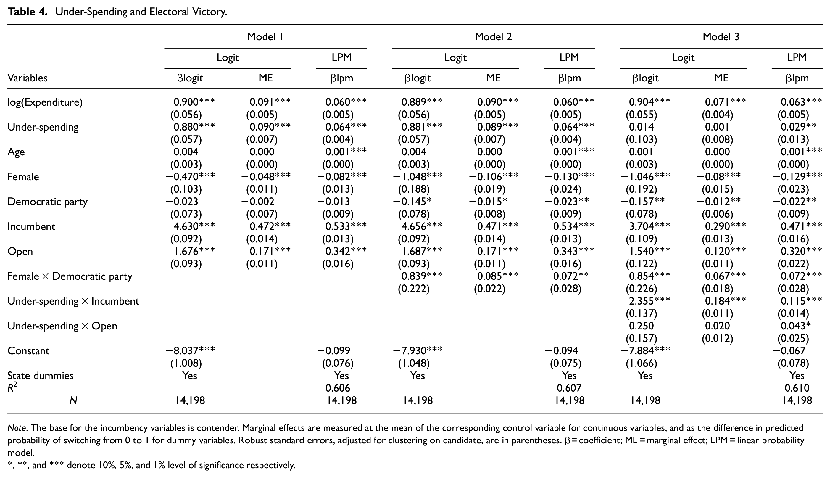
Note. The base for the incumbency variables is contender. Marginal effects are measured at the mean of the corresponding control variable for continuous variables, and as the difference in predicted probability of switching from 0 to 1 for dummy variables. Robust standard errors, adjusted for clustering on candidate, are in parentheses. β = coefficient; ME = marginal effect; LPM = linear probability model.
, **, and *** denote 10%, 5%, and 1% level of significance respectively.
Table 2 displays results of regressions based on equation (1), which examines the effect of campaign expenditure on a candidate’s probability to win a seat. All models show a positive and significant association between winning probability and the amount of money spent by candidates. In Model 1, a 1% increase in campaign expenditure corresponds to a 0.065 marginal effect, indicating that candidates are 6.5 percentage points more likely to win, all other variables held constant. Besides the expenditure variable, the categorical variables for female and incumbency status are also statistically significant. Female candidates are 4.1 percentage points less likely to win than their male counterparts. Incumbents and open candidates are roughly 46.6 and 16.9 percentage points more likely to win than contender candidates, respectively. Interestingly, age and party membership do not significantly affect the winning probability of candidates.
In Model 2, the relationship between candidates’ gender and party affiliation is scrutinized with the inclusion of an interaction term. The interesting finding is that when a female candidate runs an election under the flag of Democratic party, she is 8.3 percentage points more likely to win such an election than a female Republican candidate. Meanwhile, a male candidate from Democratic party is 1.5 percentage points less likely to win an election than his male Republican counterpart. Age continues to be an insignificant factor in affecting the election outcome.
In Model 3, the interaction between candidates’ expenditure and incumbency status is added to the regression. A significant negative marginal effect for the interaction term of expenditure-incumbent suggests that spending money is less effective for incumbents to improve their chances of winning than contenders. Holding current office, incumbents usually generate significant recognition in the US (Stone et al., 2004). Their achievements and press releases appear in newspapers regularly. They have plenty of constituency connections as part of their regular office duties. These resources are themselves campaigns for incumbents for re-election. Nevertheless, at a certain stage, the campaigning and recognition reach a point of diminishing marginal return (Bonneau & Cann, 2011). At that point, spending money can do little to increase incumbent candidates’ recognition further (Green & Krasno, 1988). On the other hand, spending is more effective for contenders due to the increasing marginal returns for each dollar spent on campaigning (see for instance, Pastine & Pastine, 2012). In this respect, our result highlights the differing effect of expenditure on the winning probability for a contender versus an incumbent. Meanwhile, campaigning is less effective in open seat elections (i.e., those in which there is no incumbent candidate involved) as evidenced by a negative and significant marginal effect for the interaction term between expenditure and open election variables. This may be because in these open elections, such a difference between contender spending and incumbent spending no longer exists.
Table 3 shows how SIGs’ contributions can affect the probability of winning for political candidates. It reports the results from the logit estimation of equation (2) as well as those from the linear probability estimation for robustness checks. It can be seen that the corresponding marginal effect for SIG contributions is positive and statistically significant across the models. As evident in both Models 1 and 2, candidates who receive an additional 1% in contributions from SIGs are approximately 5.9 percentage points more likely to secure victory, with all other factors held constant. Thus, the winning probability of a candidate will increase if SIGs contribute more to that candidate. Findings for the control variables are quite similar to the previous results from Table 2.
In Model 3, the interaction between SIG’s contributions and candidates’ incumbency status is added to the regression. Here, the probability of winning a seat increases dramatically by 16.1 percentage points for contenders but falls by 25 percentage points (equal to 16.1–41.1) for incumbents for every 1 percentage point increase in contribution from SIGs. Usually, uninformed, as well as non-partisan voters, are reluctant to cast their ballots for a contender, who is little known to them (Baron, 1994). Hence, campaign activities are crucial for contenders to achieve electoral success in comparison to incumbents. From Table 2, we have seen that contenders’ likelihood of winning increases when they spend more on campaigning. To finance this spending, they need contributions, which mostly come from SIGs. As such, the results in Table 3 are in line with those in Table 2, showing that contenders’ likelihood of winning increases if they receive more campaign contributions from SIGs. However, the negative marginal contribution effect for incumbents suggests a different story. As in Table 2, incumbents do not need to spend much on electoral campaign activities to raise their winning probability. Results in Table 3 shed further light into this picture by indicating that more contributions from SIGs do not necessarily enhance the probability of wining for incumbents.
So far, we have shown how spending and contributions for a campaign can impact the winning probability of candidates. What remains to be seen is the implication of the gap between campaign spending and contribution on candidates’ chance of being elected. Table 4 reports results from the logit regressions of equation (3) (and with linear probability results for robustness checks). Here, Under-spending is a binary variable capturing the case when campaign spending is less than contributed amount. It receives the value of 1 if spending is less than contribution and 0 otherwise. Table 4 shows a mostly positive and statistically significant relationship between this variable and election success. In particular, Model 1 and Model 2 suggest that candidates who spend less than the amount of contributions received are roughly 9 percentage points more likely to win. Given that the majority of candidates are incumbents, the law of diminishing marginal returns leads them to spend less than the total amount of SIGs’ contributions. Thus, the Under-spending dummy variable might be reflecting a strong association between incumbency and electoral success.
To gain more insight into the relationship between under-spending and candidates’ incumbency status, we add their interaction terms to the regression in Model 3. The corresponding coefficients are positive and significant for both interaction terms with incumbent candidates and open candidates. Meanwhile, the effect of under-spending for the contender is negative but statistically significant. All these suggest that while spending less than total amount of contribution received may not be a good strategy for contender candidates, this works well for incumbent and open candidates.
Addressing the Endogeneity
As discussed earlier, the monetary variables may be endogenous due to the potential reverse causality from the winning probability variable to monetary variables. In Table 5, we reproduce the regressions presented in Table 2, however, this time using the Lewbel’s (2012) method to control for the potential endogeneity of Expenditure. Given that the Lewbel’s method is only applied to linear models, in Table 5 (and other tables to follow), we will only present the IV-augmented linear regression results. Since the linear probability results produce qualitatively the same results as those obtained under the logit regressions, the Lewbel’s IV-augmented linear regression results are deemed sufficient.
Campaign Spending and Electoral Victory (Lewbel’s Method Estimation).

Note. Robust standard errors are in parentheses.
, **, and *** denote 10%, 5%, and 1% level of significance, respectively.
All F-statistics of weak identification tests are highly significant indicating relevant instruments. The estimated coefficient for log of Expenditure is positive and significant across all models. This reiterates the positive effect of campaign expenditure on candidates’ winning probability in the baseline specifications presented in Table 2. The results also validate the earlier finding that the positive effect diminishes for incumbent candidates.
With the aim of addressing the potential endogeneity between contribution amount and candidates’ probability of winning, Table 6 replicates Table 3 using Lewbel’s IV estimation method. Again, all F-statistics of weak identification test are highly significant meaning that the generated instruments are relevant. The positive effect of Contribution on candidates’ winning probability is reaffirmed in all model specifications. In addition, campaign contribution plays a more crucial role in enhancing success of contenders than incumbents in an election.
Campaign Contribution and Electoral Victory (Lewbel’s Method Estimation).
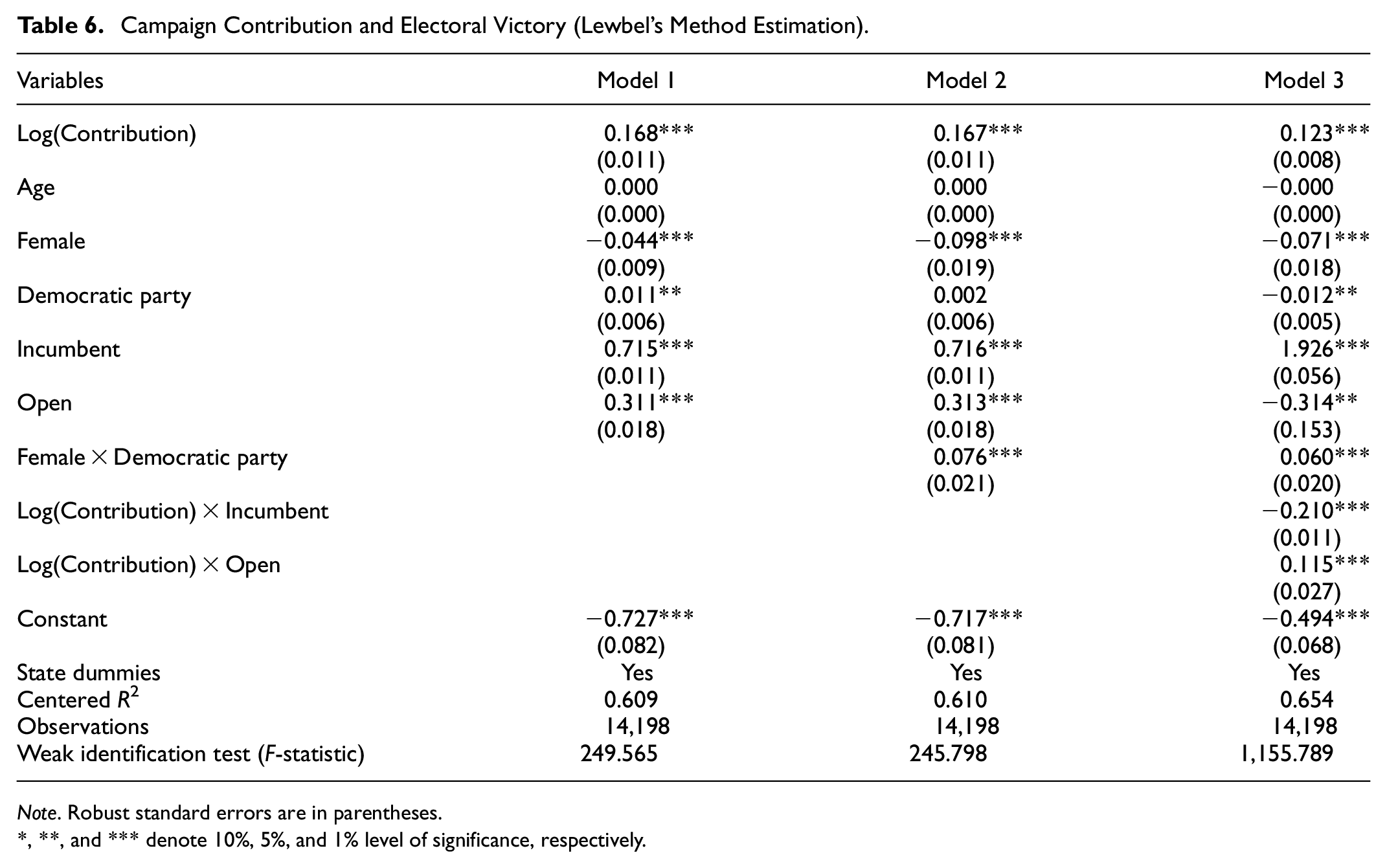
Note. Robust standard errors are in parentheses.
, **, and *** denote 10%, 5%, and 1% level of significance, respectively.
Similarly, Table 7 reproduces the results reported in Table 4 using the Lewbel’s IV estimation method. Again, F-statistics of weak identification tests are significant indicating the relevance of generated instruments. Obtained results are qualitatively similar to the baseline results with coefficients of Expenditure and Under−spending being positive for Models 1 and 2. In Model 3 we observe slight differences compared to Table 4. In particular, the interaction between Under−spending and Open is insignificant. In addition, the coefficient of Under−spending is positive and statistically insignificant (in Table 4, this coefficient is negative and insignificant). This means that even though the endogeneity problem might present in our data, it is not so severe.
Under-Spending and Electoral Victory (Lewbel (2012)’s Method Estimation).

Note. Robust standard errors are in parentheses.
, **, and *** denote 10%, 5%, and 1% level of significance, respectively.
Further Robustness Checks
In the previous section, we provided the first robustness test of our logit estimation results with the conduct of the linear probability estimation. In this section, we continue to examine the sensitivity of our results by re-estimating equations (1) to (3) using a sample of a different size. Obtained results are then compared and contrast with those previously discussed in section “Results and Discussions.”
It might be argued that in elections where there are no incumbents running for reelection (i.e., open seat elections), candidates behave differently leading to different effectiveness of monetary spending on electoral success. To accommodate this possibility, in Tables 8 to 13, we report results for regressions on a sub-sample established by excluding open elections. It can be seen that the number of observations decreases from 14,198 to 13, 095. However, obtained results are qualitatively the same as those previously included in Tables 2 to 7 in terms of signs and significance, although the marginal effects have smaller magnitudes. This may be because of the decrease in sample size when we removed all open elections. Overall, both spending and contributions for a campaign positively and significantly affect candidates’ winning probability. The effectiveness of the impact depends on candidates’ incumbency status. This implies that our results are not sensitive to the inclusion or exclusion of open seat elections.
Campaign Spending and Electoral Victory (Excluding Open Elections).

Note. The base for the incumbency variables is contender. Marginal effects are measured at the mean of the corresponding control variable for continuous variables, and as the difference in predicted probability of switching from 0 to 1 for dummy variables. Robust standard errors, adjusted for clustering on candidate, are in parentheses. β = coefficient; ME = marginal effect; LPM = linear probability model.
, **, and *** denote 10%, 5%, and 1% level of significance respectively.
Campaign Contribution and Electoral Victory (Excluding Open Elections).

Note. The base for the incumbency variables is contender. Marginal effects are measured at the mean of the corresponding control variable for continuous variables, and as the difference in predicted probability of switching from 0 to 1 for dummy variables. Robust standard errors, adjusted for clustering on candidate, are in parentheses. β = coefficient; ME = marginal effect; LPM = linear probability model.
, **, and *** denote 10%, 5%, and 1% level of significance respectively.
Under-Spending and Electoral Victory (Excluding Open Elections).
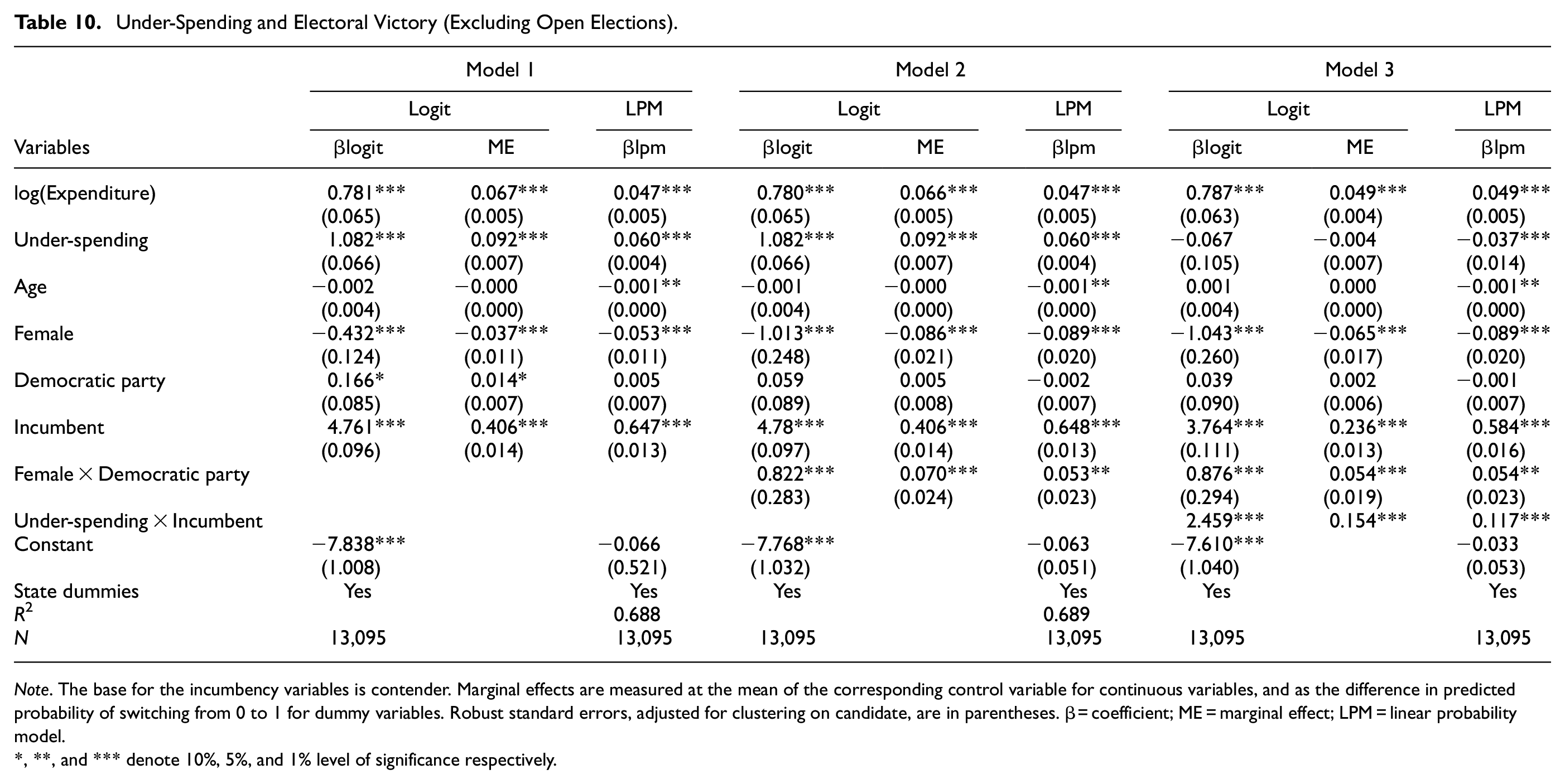
Note. The base for the incumbency variables is contender. Marginal effects are measured at the mean of the corresponding control variable for continuous variables, and as the difference in predicted probability of switching from 0 to 1 for dummy variables. Robust standard errors, adjusted for clustering on candidate, are in parentheses. β = coefficient; ME = marginal effect; LPM = linear probability model.
, **, and *** denote 10%, 5%, and 1% level of significance respectively.
Campaign Spending and Electoral Victory (Lewbel (2012)’s Method Estimation, Excluding Open Elections).

Note. Robust standard errors are in parentheses.
, **, and *** denote 10%, 5%, and 1% level of significance, respectively.
Campaign Contribution and Electoral Victory (Lewbel (2012)’s Method Estimation, Excluding Open Elections).
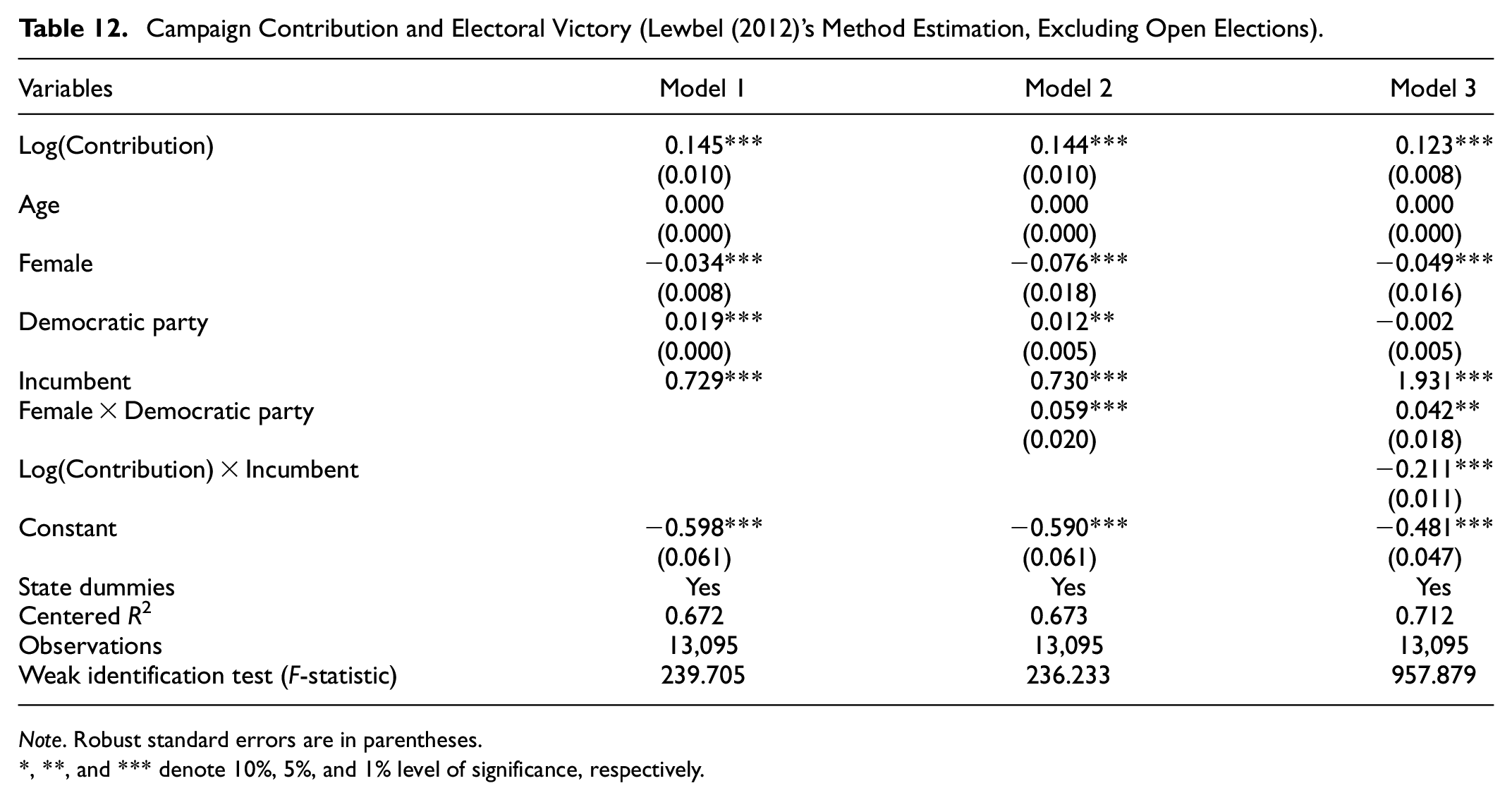
Note. Robust standard errors are in parentheses.
, **, and *** denote 10%, 5%, and 1% level of significance, respectively.
Under-Spending and Electoral Victory (Lewbel (2012)’s Method Estimation, Excluding Open Elections).

Note. Robust standard errors are in parentheses.
, **, and *** denote 10%, 5%, and 1% level of significance, respectively.
Overall, the obtained results converge to the point that money spending plays an important role in politics, particularly through its impact on electoral outcomes. Notably, the strength of the impact varies according to candidates’ incumbency status. These results are robust to different estimation methods, econometric specifications and sample sizes. The use of robust standard errors in our regressions fixes the inherent heteroscedasticity in the logit and linear probability models. In addition, having a bigger sample helps trivialize the non-normality of the standard errors.
Concluding Remarks
In this paper, we have examined how money, in the form of campaign contribution, made by SIGs, and its spending, affects electoral outcomes. We collected data on the House of Representatives elections from all 50 states and Washington D.C. in the US over the period of 2000 to 2018. Based on the logit estimations (and also the linear probability estimations), we show that campaign expenditure and electoral success are positively correlated. We also find that party membership, but not age, of candidates impacts the winning probability, whereas the impacts of gender and incumbency status are more profound. A Republican female candidate is observed to face more difficulties to win than a Democratic one. An interesting aspect of the relationship between campaign spending and winning probability is that the effectiveness of campaign expenditure varies according to different incumbency status (Benoit & Marsh, 2008). Our finding is in line with existing results in the literature regarding the US House elections that incumbent candidates gain less from spending, compared to their contender counterparts. This is due to diminishing returns that occur at a certain point, after which incumbent candidates can increase the winning probability only marginally (Green & Krasno, 1988). However, this finding is in contrast with other studies considering electoral systems in Brazil, Japan, or India, where spending effectiveness is equally applicable for both incumbents and contenders (Johnson, 2013; Lee, 2020; Samuels, 2001). Our finding, therefore, implies that incumbent candidates do not necessarily need to use up all funds they receive from donors for campaigns during an election. It signals that when incumbents get more funds from donors than what is needed for campaign expenditure, they may then enjoy the luxury of choosing how to deal with the spare money. Herrnson et al. (2019) also describe that many incumbents spend campaign funds in alternative avenues other than their own campaigns. They use it to deter potential challengers, dissuading them from entering the race. They use the resources supporting their party as well as their fellow candidates. These contributions to party entities and House candidates assist incumbents not only in ascending the ranks of House leadership but also in securing coveted committee assignments and advancing their political careers.
Generally, all candidates, including incumbents and contenders, ask for contributions from different interest groups to finance their electoral advertisements (Ashworth, 2006). In exchange for the contributions, candidates promise to do favors for the contributors if they get elected. As with the previous literature, contributors believe that it is more attractive to invest in incumbents than in contenders due to two different reasons (Ashworth, 2006; Benoit & Marsh, 2008; Johnson, 2013). Firstly, incumbents already have established name recognition and benefited substantially from prior office holding strategies and stronger networks. Therefore, they usually have a better chance of winning. The present study has empirically shown that higher campaign spending does not help incumbents much to secure a seat. Hence, incumbents do not have as much a demand for SIGs’ contributions as contenders do. Secondly, interest groups find contenders less advantageous to start with as their winning chance is uncertain. This is also shown by our results. Moreover, because the accessibility of contenders to uninformed voters is more expensive, the outcome of contributing the same amount of money to contenders is more uncertain than incumbents (Bombardini & Trebbi, 2011). Therefore, SIGs tend to supply more contributions to incumbents than contenders. This can create an overflow of funds for incumbents. This overflow may lead to incumbents’ expropriation of public resources for their personal purposes rather than election (see, for instance, Le & Yalcin, 2018, 2023a, 2023b). Moreover, it can facilitate the entrenchment of incumbents in their positions by distorting policy to suit donor preferences. In that respect, incumbents’ alternative ways of using the spare funds that they receive from SIGs are clearly not in the public interest and should be regulated. Examining these issues, either theoretically or with data, will enrich our forthcoming research agenda. In the future, we may explore the possibility of incorporating spatial econometrics techniques into our analysis to consider potential spatial spillover effects. In the context of election campaign spending, using spatial econometrics can help analyzing the interdependence of campaign spending decisions across geographically adjacent electoral districts. This can lead to more insightful analyses of how campaign funds are distributed and the impact of spending in one district on neighboring districts. Another future research direction is to include in the model factors that potentially influence fund-raising, spending and outcomes such as seniority and leadership positions of incumbents or political experience of contenders and open-seat candidates when such kind of information is available.
Footnotes
Declaration of Conflicting Interests
The author(s) declared no potential conflicts of interest with respect to the research, authorship, and/or publication of this article.
Funding
The author(s) received no financial support for the research, authorship, and/or publication of this article.
Data Availability Statement
Data sharing not applicable to this article as no datasets were generated or analyzed during the current study.