Sage Journals: Discover world-class research

Abstract

Most of the macro-literature on uncertainty has focused on macro-uncertainty caused by real activity as a source of economic fluctuations. Economic uncertainty reduces total demand in the economy via a conventional channel that is associated with real option theory. Given the findings of the existing literature, financial uncertainty other than macroeconomic uncertainty matters more for business cycle fluctuations. This study seeks to answer the following questions: Is uncertainty the primary cause of the business cycle’s fluctuations? Alternatively, does it matter what kind of uncertainty exists? The research utilized the generalized linear model (GLM) and the Bayesian generalized linear model (BGLM) to analyze a dataset covering the time from July 1960 to April 2015 in the United States. Elevated levels of macroeconomic uncertainty, akin to real uncertainty, and economic policy uncertainty, as measured by news sources, demonstrate a counter-cyclical pattern in relation to business cycles. Low levels of uncertainty have a positive impact on business cycles, leading to an increase in industrial production. Conversely, high levels of uncertainty have a negative effect on business cycles, causing a decline in industrial output. We are of the opinion that high levels of macroeconomic uncertainty have a ripple effect on the entire economy, which may stifle investments, reduce consumption, and create unemployment, which is likely to influence labor participation.

JEL Classification: D81, E23, E32, E44, G14.

Plain Language Summary

Financial and macroeconomic uncertainty impact on business cycles

Purpose: Most of the macro literature on uncertainty has focused on macro uncertainty caused by real activity as a source of economic fluctuations. Economic uncertainty reduces total demand in the economy via a conventional channel that is associated with the real option theory. Given the findings of the existing literature that financial uncertainty other than macroeconomic uncertainty matters more for business cycle fluctuations. This study seeks to answer the following questions: is uncertainty the primary cause of the business cycle’s fluctuations? Alternatively, does it matter what kind of uncertainty exists? Methods: We use the GLM and Bayesian GLM as well as the Granger causality test on monthly frequency data spanning 1960:07 to 2015:4. Conclusions: Numerous estimations employing diverse measures of uncertainty lead us to the conclusion that high levels of macroeconomic uncertainty, which is comparable to real uncertainty, exhibit counter-cyclical behavior with respect to business cycles as well as economic policy uncertainty as measured by news. Business cycles respond favorably to low levels of uncertainty, which supports an increase in industrial production but negatively to high levels of uncertainty, resulting in decreased industrial output. Implication: This observation strongly indicates the presence of an inverted U-shaped relationship between macroeconomic uncertainty and business cycles, while a linear relationship is observed between financial uncertainty and industrial production. Elevated levels of uncertainty possess the potential to disrupt the natural progression of business cycles and consequently diminish industrial production.

Keywords

financial uncertainty macroeconomic uncertainty economic policy uncertainty real uncertainty business cycles industrial production

Introduction

A strand of literature in macroeconomics investigates the interaction between uncertainty and business cycle fluctuations. The increasing evidence suggests that recessions are accompanied by a significant increase in uncertainty, which has heightened interest in the subject; see, for example, Born and Pfeifer (2021) and Ludvigson et al. (2021). These findings are supported by the use of proxy variables like stock market volatility and forecast dispersion (Bloom, 2009), or a broad-based measure of macroeconomic uncertainty is used (Jurado et al., 2015). Even though this evidence supports the notion that uncertainty plays a role in severe recessions, the question of whether low or high levels of uncertainty are a source of business cycle fluctuations or responses to economic fundamentals is not fully understood.

There has been a resurgence of research interest in the field of economic uncertainty modeling and its significance in forecasting macroeconomic fluctuations in recent years (Al-Thaqeb & Algharabali, 2019; Junttila & Vataja, 2018; Nowzohour & Stracca, 2020). During financial crisis periods, the spread of negative news lowers expectations for future economic activity, leading to the occurrence of economic uncertainty. The United States experienced a notable spike in macroeconomic and financial uncertainty during the global financial crisis (Born et al., 2018; Choudhry et al., 2020a; Leduc & Liu, 2020), and the conventional causes of fluctuations in business cycles (BCs) have been called into question as a result of the global financial crisis. Recent research has indicated that economic uncertainty can serve as an alternative catalyst for economic fluctuations (Cerra et al., 2023; Choudhry et al., 2020a; Dew-Becker & Giglio, 2023; Ludvigson et al., 2021; Trung, 2019).

According to Cascaldi-Garcia et al. (2023), uncertainty is becoming an increasingly important factor for empirical research in a variety of economic applications. According to the findings of an early study by Bernanke (1983), an increase in economic uncertainty reduces total demand in the economy via a conventional channel that is associated with the real option theory. It has been hypothesized that uncertainty influences decision-making because it raises the value of waiting as an option; see Lee and Daunizeau (2020) and Lees et al. (2022). When faced with uncertainty, businesses and, in the case of long-lasting products, consumers are more likely to exercise extreme caution in order to avoid the significant financial losses that are associated with making poor investment decisions (Dreyer & Schulz, 2023; Khan et al., 2020; Wen et al., 2021). As a result, businesses and consumers delay making decisions about investments, employment, and spending until uncertainty decreases. Uncertainty is expected to negatively influence the supply-side productivity of the economy due to the misallocation of resources across businesses (Bloom et al., 2018). For example, Bloom et al. (2018) assert that during normal times, inefficient companies contract while productive firms expand, which helps to maintain high aggregate productivity. This, in turn, helps to maintain a high level of employment overall. Businesses are more likely to restrict their expansion and contraction plans when there is a high level of uncertainty because doing so stifles a significant portion of this productivity-enhancing reallocation. This, in turn, leads to a decline in measured aggregate total factor productivity.

Even though uncertainty measures have a strong correlation with financial market variables, existing findings are based on practical but limited identifying assumptions and do not address financial markets explicitly. This paper makes several assumptions to distinguish between the causes and effects of macroeconomic and financial uncertainty, as well as other measures of uncertainty’s impact on business cycles. Generally, the uncertainty literature struggles with the issue of causality and determining high and low uncertainty. As a result, there is no theoretical consensus on whether the uncertainty associated with deep recessions is primarily a cause or an effect (or both) of economic activity declines. This presents a problem. In fact, the direction of the effect is unclear in the theory. It is difficult to analyze the role of uncertainty in business cycle fluctuations econometrically. To identify the effects of uncertainty shocks, existing empirical work primarily relies on recursive schemes within the framework of vector autoregressions (VAR); see, for example Bloom (2009), Gilchrist et al. (2014), and Jurado et al. (2015). A recursive structure is a quick and easy way to start looking into the relationship between uncertainty and business cycles, but it does not provide a satisfactory solution. There is no compelling theoretical reason to limit the timing of uncertainty’s relationship with real activity, which is a first-moment variable, and the former, a second moment variable.

Furthermore, existing studies disagree on whether uncertainty in the VAR should come before or after real activity variables. Given that uncertainty is both an exogenous impulse determinant of business cycles and an endogenous response to first-moment shocks, it can fluctuate concurrently with real activity. With recursive structures, which assume delayed responses from some variables, this is obviously impossible; see Ludvigson et al. (2021). Many methods for identifying VARs, including but not limited to long-run restrictions, sign restrictions, and instrumental variable estimation, are problematic. Given the above argument, we contribute to the existing literature by using the generalized linear model (GLM) and Bayesian generalized linear model (Bayes GLM) to answer the question: is uncertainty the primary cause of the business cycles’ fluctuations? Alternatively, does it matter what kind of uncertainty exists? By using these methods, we are better able to capture the non-normal distribution of the errors in the data series, and perhaps the function that connects the predictor to the response may be specified (see, e.g., Gunst, 1984; McCullagh, 1989; McCulloch, 2000; Myers & Montgomery, 1997; Nelder & Wedderburn, 1972; Neter et al., 1983).

Additionally, we assess the relationship between uncertainties and business cycles under high and low assumptions using the quadratic terms of the variables, which is different from the existing literature; see Bloom (2009), Jurado et al. (2015), Bloom et al. (2018), and Ludvigson et al. (2021). We motivate our model with the EKC model, which suggests that there is an inverted U-shaped curve between the environment and affluence; see for example, Grossman and Krueger (1995), Ulucak and Bilgili (2018). In this situation, elevated levels of income tend to reduce environmental degradation. The quadratic term of GDP measures elevated levels of income. In a similar vein, the inflection point of uncertainty is the value at which the quadratic effect changes direction. This point is where the curve transitions from increasing to decreasing. Numerous studies have used the quadratic term of variables such as total assets (Gadzo et al., 2019; Guerard & Mark, 2003; Kalu et al., 2016), income levels (Chen et al., 2023; Ciarlantini et al., 2023; Zhao et al., 2016, among many others), etc. to measure the inflection point of curve transitions from increasing to decreasing effects on other variables. We assume that at the initial stages of the business cycle, uncertainty causes a boom in industrial production and that, in later stages of the business cycle, elevated levels of uncertainty cause a bust in industrial production after uncertainty reaches a turning point. It implies that the business cycle first booms and then busts, with an increase in uncertainty. Conducting this study aims to enhance our understanding of the economic dynamics that occur during times of uncertainty. Additionally, it aims to offer practical guidance to diverse stakeholders on effectively managing and responding to economic challenges. Through the acknowledgment and examination of the identified constraints, this study has the potential to yield significant contributions to the fields of economics and finance, encompassing conceptual and applied dimensions.

Our key findings are: (1) that high levels of macroeconomic uncertainty matter more than financial uncertainty, despite our findings indicating that low levels of financial and macroeconomic uncertainties are significant and positive drivers of industrial production.

(2) High levels of macroeconomic uncertainty, which is comparable to real uncertainty, exhibit counter-cyclical behavior with respect to business cycles as well as economic policy uncertainty as measured by news. Business cycles respond favorably to low levels of uncertainty, which supports an increase in industrial production, but negatively to high levels of uncertainty, resulting in decreased industrial output. These findings strongly suggest an inverted U-shaped relationship between macroeconomic uncertainty and business cycles, while financial uncertainty shows a linear relationship with industrial production. We are of the opinion that high levels of macroeconomic uncertainty have a ripple effect on the entire economy, which may stifle investments, reduce consumption, and create unemployment, which is likely to influence labor participation.

The study is divided into five sections: section one introduces the topic and the motivation; section two briefly discusses the existing literature on the topic; section three describes the empirical methods used; section four presents the empirical results; and section five concludes the study.

Brief Literature Review

As a possible factor in business cycles, uncertainty has received considerable attention. According to Bloom et al. (2018), uncertainty shocks generally result in a 2.5% decline in GDP, followed by a rapid recovery and a continuation of the output slowdown. This suggests that uncertainty may be a significant factor in business cycle initiation or amplification. In addition, the authors find that the economy responds significantly less positively to stimulative policies as firms become cautious in the face of uncertainty. In contrast to financial market uncertainty, which is likely a source of output fluctuations, Ludvigson et al. (2021) find that greatly elevated macroeconomic uncertainty is frequently an endogenous response to production shocks in recessions. Similarly, Baker et al. (2020) embarked on a cross-country study using a VAR setting under diverse assumptions and restrictions. They concluded that financial uncertainty greatly exacerbates economic growth. Given that uncertainty increases during recessions and decreases during boom cycles. Contrarily, in a theoretical model, Born and Pfeifer (2021) predict with high confidence that the quantitative impact of uncertainty shocks on the economy is negligible.

In a previous study, Nakamura et al. (2017) showed that for a panel of 16 developed economies, uncertainty and real economic activity have an adverse relationship. On the issue of whether this correlation suggests that uncertainty is primarily a cause or a result of declines in economic activity, theories for which uncertainty plays a key role vary greatly. The empirical analysis of the U.S. business cycle has been the primary focus of some studies. Most of these studies concluded that heightened uncertainty significantly dampens economic activity, resulting in decreased output, decreased consumer spending, decreased investment, and increased unemployment. These results are consistent across a wide variety of uncertainty proxies, including financial volatility indexes (Bloom, 2009), measures of macroeconomic uncertainty, and news-based indices of political uncertainty (Baker et al., 2016; Jurado et al., 2015; Lakshmi et al., 2019; Ludvigson et al., 2021, among many others).

The literature on uncertainty raises a separate issue regarding the genesis of uncertainty. According to conventional theories, uncertainty stems from economic fundamentals such as productivity and is deterred by market frictions when it interacts with real economic uncertainty; see Bonciani and Ricci (2020). Nonetheless, a number of scholars contend that uncertainty weakens the economy by affecting financial markets or by posing specific financial market-specific risks (Bollerslev et al., 2009; Gilchrist et al., 2014; Liu, 2021; Z. Li & Zhong, 2020). Furthermore, Ng and Wright (2013), found that all recessions since 1982 can be attributed to the financial markets, and these recessions exhibit notable distinctions from those where the financial markets played a secondary role. If financial shocks are subject to time-varying volatility, financial market uncertainty, as opposed to real economic uncertainty, could be a significant contributor to recessions, both as a cause and a transmission mechanism. However, the literature has sparsely distinguished how real versus financial uncertainty influences business cycle fluctuations.

According to a body of research, uncertainty contributes to slower economic growth. These studies include those that investigate how uncertainty affects real options, those that investigate how uncertainty affects financial constraints, and those that investigate precautionary saving (Arellano et al., 2010; Basu & Bundick, 2017; Bernanke, 1983; Fernández-Villaverde et al., 2011; Gilchrist et al., 2014; Leduc & Liu, 2016; Z. Li & Zhong, 2020; McDonald & Siegel, 1986). These theories almost universally assume that uncertainty externally perturbs the volatility of economic fundamentals. Some theories posit that an increase in uncertainty is a direct consequence of the process governing technological innovation, which then leads to a decline in actual activity; see Bloom (2009) and Bloom et al. (2018). Heightened macro uncertainty, according to these theories, should reduce real economic activity. Despite the theoretical literature’s emphasis on uncertainty stemming from economic fundamentals, the empirical literature has typically evaluated these theories using uncertainty proxies that are highly correlated with financial market variables. This practice raises the intriguing question of whether recessions are the result of real economic uncertainty, financial market uncertainty, or both.

Slower economic growth, according to a second school of thought in the literature, is the sole cause of the rise in macroeconomic uncertainty. There is no exogenous uncertainty relationship in these theories, and all uncertainty variation is endogenous. Unfavorable economic conditions, according to some theories, encourage risky behavior, reduce information and, as a result, make future events less predictable, and resulting in novel economic policies with unpredictable outcomes (see Bachmann et al., 2013; Fajgelbaum et al., 2017; Fostel & Geanakoplos, 2012; Ilut & Saijo, 2021; Pástor & Veronesi, 2013; Van Nieuwerburgh & Veldkamp, 2006).

Other researchers, however, contend that certain types of uncertainty may even stimulate the economy. According to the growth options uncertainty theories, businesses may make investments and hire employees if there is a risk spread that is mean-preserving. This risk spread results from an unbounded upside and a constrained downside, which in turn raises expected profits due to the increased mean-preserving risk. Frequent advancement of these explanations characterized the dot-com boom. Early studies include those from Oi (1961), Hartman (1972), and Abel (1983), as well as more recent works by Bar-Ilan and Strange (1996), Pástor and Veronesi (2013), Segal et al. (2015) and Kraft et al. (2018). These studies show that data cannot be related to by a single uncertainty theory or all-encompassing structural model. Simply put, the body of theoretical work lacks sufficient specific identification constraints for empirical research. Instead, the literature offers a variety of theoretical hypotheses, all of which are ambiguous about the nature of the relationship between uncertainty and real economic activity. The lack of theoretical agreement on this relationship, as well as the multiplicity of theories and a lack of information on the structural elements of specific models, highlight the fundamental nature of empirical cause-and-effect analysis.

Ali et al. (2023) conducted a thorough analysis from a governance standpoint to assess the effects of economic policy uncertainty (EPU) on the stability of the financial system. The research conducted by the authors produced significant results, demonstrating that the implementation of efficient governance mechanisms can be an effective strategy for reducing the negative impacts of economic policy uncertainty (EPU) on the stability of financial systems. However, the extent to which regional disparities, the banking institutions involved, and the distinct structural characteristics of financial markets influenced the observation of this mitigating factor varied significantly. The study revealed a significant phenomenon, suggesting that the positive effect of governance on financial stability concerns caused by economic policy uncertainty was particularly strong during the turbulent period of the global financial crisis.

Macroeconomic and financial uncertainty, as well as industrial production, impact the management of volatility, stock market returns, and commodity prices; see Demir and Ersan (2017), Chowdhury et al. (2021), Zhang et al. (2022). By regulating inflation, bolstering consumer confidence, mitigating systemic risk, promoting long-term investment, and contributing to global competitiveness, it aids in the preservation of economic stability (Volpin & Maximiano, 2020; Wang et al., 2023). Stable commodity prices facilitate monetary policy transmission, enabling central banks to execute policies with greater efficacy (Carriere-Swallow et al., 2016; Johnson et al., 2020; Yellen, 2015). Additionally, stable markets facilitate investment and business planning, which increases production and expansion expenditures; see also O'connor (2017) and Kirschen and Strbac (2018). Additionally, job growth and consistent consumer spending are outcomes that ensue from stable economic environments (Chetty et al., 2020; Ganong & Noel, 2019). The regulation of stock market volatility and returns serves as a preventive measure against speculative bubbles and financial crises (Wuthisatian & Thanetsunthorn, 2018; Yang, 2017). In general, the regulation of these variables enhances the stability of the economic system.

Uncertainty in the US

Numerous instances of significant financial instability have occurred in the United States over time, including the 1987 stock market crash and the Great Financial Crisis or Great Recession of 2008–2009 (Afonso & Blanco-Arana, 2022; Vidal, 2021). On Monday, October 19, 1987, the Dow Jones Industrial Average experienced its largest one-day decline ever, falling 22.6% (Ajayi et al., 2020; Ludvigson et al., 2021). Popular explanations include the accelerating globalization of financial markets and financial innovations such as portfolio insurance and index futures. As a result of the widespread belief that these financial innovations were a significant cause of the crash, new rules for exchange trading, such as circuit breakers, and revised trade clearing procedures were enacted; see Ludvigson et al. (2021).

The Dow Jones Industrial Average began a precipitous decline in October 2008 and fell more than 50% over a period of 17 months. Researchers frequently cite the widespread Great Financial Crisis (GFC) as the trigger of the Great Recession (GR) (Afonso & Blanco-Arana, 2022; Ludvigson et al., 2021; Vidal, 2021). Numerous potential causes of the crisis have been identified, including problems with subprime lending and a prior housing boom. However, at least a portion of the variance in financial uncertainty appears to stem from the securities markets. Financial intermediaries played a significant role in the financial crisis, primarily due to the fact that they hold vast portfolios of financial securities. Some analyses have placed speculative trading activities by large financial institutions like AIG, Lehman Brothers, and Bear Stearns at the center of the crisis; see Glaeser et al. (2019).

Prior to the recession, several highly leveraged financial institutions, such as BNP Paribas and Northern Rock, went through a complete collapse of liquidity starting in August 2007. Uncertainty about the value of new financial innovations, such as the securitization of mortgages and other debt obligations and the explosive growth of credit default swaps, has been linked to the financial crisis. In summary, the fact that factors specifically from financial markets appeared to play a significant role in increased financial uncertainty is a distinguishing characteristic of both the 1987 crash and the GFC. In light of this, we investigate the potential impact of uncertainties on business cycles. To answer this question, we’ve constructed models to better comprehend the phenomenon.

Empirical Methods/Data

Data Sources

The data used in this study were sourced from Ludvigson et al. (2021). Macroeconomic and financial uncertainties are based on statistical uncertainty indices based on Jurado et al. (2015) methodology. The frequency of the data is monthly, and the series with full data starts from 1960:07 to 2015:4. Business cycles are the dependent variable, is measured by industrial production which has been considerably used in the literature to measure industrial output relative to real economic activity. We control for gold commodity prices, economic volatility, and stock market returns using the log difference of gold price level deflated using CPI, considering January 2018 as the base year, the Center for Research in Securities Prices (CRSP) weighted value of stock market index returns and the CBOE volatility index. For more details about the statistical underpinning of the measures of uncertainties relative to financial and macroeconomic variables, see Ludvigson et al. (2021). We also used other measures of uncertainty in the literature, such as the economic policy uncertainty index and the economic policy uncertainty news-based index constructed by Baker et al. (2016). The availability of data of these indices ranges from 1987:01 to 2017:06. Additionally, we employ real uncertainty, a subindex for macro uncertainty that fluctuates solely due to the uncertainty in the 73 real activity variables of the macro dataset. Table 1 presents the variables used and their descriptions.

Table 1.

Variables and Data Sources.

Variables	Indicators	Units of Measurement	Sources
Industrial production	IP	Measures business cycles:	Ludvigson et al. (2021)
Financial uncertainty	FU	Statistical uncertainty index for 148 financial indicators time series	"
Macroeconomic uncertainty	MU	Statistical uncertainty index for 134 macroeconomic time series	"
Real uncertainty	RU	Subindex of macroeconomic uncertainty consisting of 73 real activity variables	"
Economic policy uncertainty	EPU	Policy uncertainty data series are based on Baker et al. (2016)	"
Economic policy uncertainty news-based	EPU_N	Policy uncertainty news-based data series are based on Baker et al. (2016)	"
Quadratic term of financial uncertainty	FU²	Square root of financial uncertainty index	"
Quadratic term of macroeconomic uncertainty	MU²	Square root of macroeconomic uncertainty index	"
Quadratic term of real uncertainty	RU²	Square root of real uncertainty index	"
Quadratic term of economic policy uncertainty	EPU²	Square root of economic policy uncertainty index	"
Quadratic term of economic policy uncertainty news-based	EPU²_N	Square root of economic policy uncertainty news-based index	"
Gold commodity price levels	GOLD	Daily auction prices of gold deflated using the Consumer Price Index	"
Stock market returns	CRSP	Center for Research in Securities Prices value-weighted stock market index return	"
Volatility	VIX	CBOE Volatility Index	"

Empirical Strategy

Empirical Model

We follow Ludvigson et al. (2021) to build the following models to critically assess the impact of financial and macroeconomic uncertainties or more broadly uncertainties, on business cycles.

\begin{matrix} I P_{t} = β_{0} + I P_{t - 11} + β_{1} F U_{t} + β_{2} M U_{t} \\ + β_{3} GOL D_{t} + β_{4} CRS P_{t} + β_{5} VI X_{t} + ϵ_{t} \end{matrix}

(1)

\begin{matrix} I P_{t} = β_{0} + I P_{t - 11} + β_{1} {FU}_{t}^{2} + β_{2} {MU}_{t}^{2} \\ + β_{3} GOL D_{t} + β_{4} CRS P_{t} + β_{5} VI X_{t} + ϵ_{t} \end{matrix}

(2)

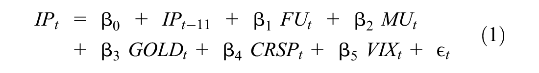
Additionally, we modeled different measures of uncertainty to robust check the macroeconomic and financial uncertainties’ measures, hence:

\begin{matrix} I P_{t} = β_{0} + I P_{t - 11} + β_{1} EP U_{t} + β_{2} EP U_{Nt} \\ + β_{3} GOL D_{t} + β_{4} CRS P_{t} + β_{5} VI X_{t} + ϵ_{t} \end{matrix}

(3)

\begin{array}{l} I P_{t} = β_{0} + I P_{t - 11} + β_{1} E P U_{t}^{2} + β_{2} E P U_{N t}^{2} \\ + β_{3} G O L D_{t} + β_{4} C R S P_{t} + β_{5} V I X_{t} + ϵ_{t} \end{array}

(4)

\begin{matrix} I P_{t} = β_{0} + I P_{t - 11} + β_{1} R U_{t} + β_{2} GOL D_{t} \\ + β_{3} CRS P_{t} + β_{4} VI X_{t} + ϵ_{t} \end{matrix}

(5)

\begin{matrix} I P_{t} = β_{0} + I P_{t - 11} + β_{1} {RU}_{t}^{2} + β_{2} GOL D_{t} \\ + β_{3} CRS P_{t} + β_{4} VI X_{t} + ϵ_{t} \end{matrix}

(6)

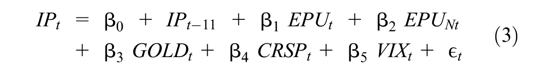
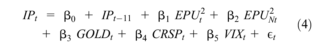
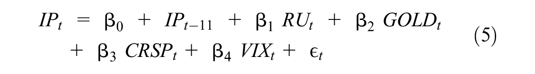
In Equations 1 to 6, $β_{0}$ denote the constant term of the slope, β₁ to β₄ represent the parameter coefficients to be estimated, $ϵ t$ denote the stochastic error terms or disturbances in the model and $t$ represent the time period for the study. RU, FU, MU, EPU, EPU_N, denote real uncertainty, financial uncertainty, macroeconomic uncertainty, economic policy uncertainty, and economic policy uncertainty news-based, correspondingly.

RU², FU², MU², EPU², EPU²_N are the quadratic terms of real uncertainty, financial un-certainty, macroeconomic uncertainty, economic policy uncertainty, and economic policy uncertainty news-based which measure heightened uncertainties.

Given the above models, we assume that it is helpful to differentiate between scenarios of heightened financial and macroeconomic uncertainty and what we will refer to as high levels of uncertainty because we are interested in determining the potential role of different types of uncertainty in economic fluctuations.

Empirical Methods

Unit Root Tests

Checks for stationarity are crucial for ensuring the accuracy of time series data. This check is essential due to the potential for inconsistency and erroneous regression estimates when using time series variables that lack stationarity. We subjected all series to a stationarity test using the Phillips and Perron (PP) test developed by Phillips and Perron (1988) and the Augmented Dickey-Fuller (ADF) test developed by Dickey and Fuller (1979). Instead of using additional lags of the first-differenced variable in the augmented Dickey- Fuller (ADF) test employed by Dickey and Fuller (1979), Phillips and Perron (1988)’s test accounts for serial correlation using Newey-West standard errors. To make the series more resistant to stationarity, we employ these two distinct testing procedures. The unit-root tests suggest that a variable is subject to a unit-root process. The null hypothesis states that the variable has a unit root, while the alternative hypothesis suggests that it is produced by a stationary process. Additionally, we performed a portmanteau white-noise test to augment the tests. We aim to capture the existence of white noise in the process of assessing the unit root in the data series; see for example, Zhu et al. (2017), Diggle (1990) and Ljung and Box (1978).

Correlations and Multicollinearity Tests

Generally, time series data consists of observations recorded across a series of time points. Tests of correlation allow us to examine the strength and direction of the relationship between two variables at various time lags; see Broock et al. (1996) and Rovine and von Eye (1997). By calculating correlation coefficients, we can determine whether variables have a linear relationship and gain insight into their interdependence. When developing time series models, it is essential to evaluate the model’s assumptions and determine their validity. The residuals (i.e., the differences between the observed values and the predicted values from the model) can be evaluated for residual correlations using correlation tests (Durbin & Watson, 1971). If significant correlations are found, it suggests that the model may not adequately capture all the pertinent data information, necessitating adjustments, see BlLLINGS and Voon (1986). Therefore, we test for correlations among the study’s variables to understand the nature of the variables over the sample period.

All regression analyses have the potential issue of multicollinearity (Thompson et al., 2017). However, multicollinearity analysis is crucially important. There are various ways to evaluate multicollinearity; see Seethaler et al. (2012). The variance inflation factor is one such diagnostic for multicollinearity. One of the most important steps in assessing the efficacy of a regression model is determining the independence of the predictors (Gunst, 1984; Neter et al., 1983). Strong predictor interdependence, or multicollinearity, has the potential to affect regression results and make our inferences more difficult; see Belsley et al. (2005). In light of this, we perform the variance inflation factor to ascertain their level of tolerance in the respective models designated for the study.

Long-Run Estimations: Generalized Linear Model

In many different fields of study, situations where the observations are not normally distributed frequently occur; see for example Myers and Montgomery (1997), Blough et al. (1999), S. Li et al. (2023), Xia et al. (2023), Yin et al. (2023) among many others. Analyzing such responses typically entails changing the response into a new quantity that behaves more like a typical random variable. Using a generalized linear model (GLM) based analysis procedure, where a non-normal error distribution and a function that connects the predictor to the response may be specified, is an alternative strategy (Myers & Montgomery, 1997). Given the nature of our data series, we find it statistically useful to employ the GLM to deal with the non-normal error distribution; see Table 2. The skewness, kurtosis, and the joint tests suggest that the error distributions are not normally distributed, as we find the p-values to be less than 5%. By using reparameterization to induce linearity and allowing a non-constant variance to be directly incorporated into the analysis, generalized linear models naturally address these problems; see Hastie and Pregibon (2017).

Table 2.

Test for Normality.

	Skewness	Kurtosis	Joint test: Adj. Chi²
IP	0.52	0.00	55.10***
FU	0.02	0.03	9.57**
MU	0.00	0.00	93.64***
RU	0.00	0.00	64.88***
EPU	0.01	0.02	10.77**
EPU_N	0.00	0.53	9.36**
GOLD	0.00	0.00	37.54***
CRSP	0.00	0.00	114.53***
VIX	0.00	0.86	12.44***
FU²	0.00	0.00	143.61***
MU²	0.26	0.03	6.12**
RU²	0.01	0.20	8.91**
EPU²	0.00	0.14	12.52**
EPU²_N	0.00	0.17	18.81***

Note. *** and ** denote p-values of 1% and 5%. These p-values suggest that the null hypothesis of normality is rejected. To put it differently, the errors distributions of the data series are in non-normal.

There may be a need for inference techniques that are not based on ordinary least squares (OLS), given the realization that many statistical modeling and analysis issues are clearly expressed in non-normal error assumptions (Lindsey, 2000; McCulloch, 2000; Myers & Montgomery, 1997; Neuhaus & McCulloch, 2011). The assumptions of normality and homogeneous variance play a significant role in the optimality characteristics of least squares estimators. To address applications involving binomial responses (proportion of defective data), poisson responses (count data—number of defects), or exponential responses (time to failure data), alternative approaches are required. There are numerous industries in which concepts or regressor variables influence the conditions that result in such responses. Nelder and Wedderburn (1972) developed the concept of generalized linear models (GLM), which McCullagh (1989) then extensively covered. This method enables regression modeling when responses are distributed based on an exponential relationship.

As previously stated, using ordinary least squares when dealing with binomial or poisson responses is inappropriate. These are only two of the numerous distributions in which the variance is dependent on the mean; therefore, any reasonable estimation procedure must take the error distribution and consequently the non-homogeneous variance into account. We will now discuss a unified family of widely applied distributions and models in the real world. This family of generalized linear models includes the normal distribution/linear model as a special case. The exponential family provides key characteristics of the normal, binomial, and Poisson distributions and relates the distribution mean to the natural location parameter. However, the exponential family did not establish a direct connection to regressor variables or regression models at that time. The set of regressor variables x_l, x₂, …, x_k are introduced via the linear predictor $x' β = β_{0} + β_{1} x_{1} + β_{2} x_{2} + . . . + β_{k} x_{k}$ . The linear predictor comprises the regression portion of the model. The relationship between the assumed distribution means and the linear predictor is utilized to construct the entire model.

This closely resembles standard normal theory linear modeling, in which we have:

E [y] = μ = β_{0} + β_{1} x_{1} + β_{2} x_{2} + . . . + β_{k} x_{k}

(7)

which Equation 7 follows

μ = x' β

(8)

The model in Equation 8 is a special case of the GLM approach, as we shall illustrate. Typically, a link function determines the relationship between the population mean and the linear predictor:

s (μ) = x' β

(9)

where s(·) is a monotonic function. The population mean is the parametric response of the regression model in Equation 9, which is obtained by:

μ = s^{- 1} (x' β)

(10)

This study’s GLM methodology is supported by the identity link, which is a link function that leads to the model in Equation 10.

Long-Run Estimations: Bayesian Generalized Linear Model

Having used a frequentist approach, that is, GLM, as our benchmark method, we employed a Bayesian GLM as a robustness check to infer our findings with confidence. Assuming that all model parameters are random variables, Bayesian analysis can incorporate prior knowledge. This assumption stands in stark contrast to more traditional statistical inference, also known as frequentist, which assumes that all parameters are unknown but constant quantities. Bayesian analysis is based on the Bayes rule, which provides a formal method for combining prior knowledge with evidence from the available data. The Bayes rule generates the so-called posterior distribution of model parameters. Incorporating new evidence from observed data into the prior knowledge of the model parameters derives the posterior distribution.

The standard estimation method for the GLM is maximum likelihood. We assume, for simplicity’s sake, that ϕ_i are unknown and X^T = (x₁, …, x_n) has rank $p$ . The formula for the likelihood function is:

L (b) \infty \exp [\sum_{i = 1}^{n} a^{- 1} (ϕ_{i}) {y_{i} h (x_{i}^{T} b) - ψ (h (x_{i}^{T} b))}]

(11)

In the Bayesian model, a prior $b$ is associated with the corresponding likelihood in Equation 11. A common option is $N (b_{0}, Σ)$ , where $b_{0}$ and $Σ$ are already known. The posterior of $b$ can be calculated by writing $y = (y_{1}, \dots, y_{n}) T$ :

\begin{matrix} (b | y) \infty \exp \\ [\sum_{i = 1}^{n} a^{- 1} (ϕ_{i}) {y_{i} h (x_{i}^{T} b) - ψ (h (x_{i}^{T} b))} - \frac{1}{2} {(b - b_{0})}^{T} Σ^{- 1} (b - b_{0})] \end{matrix}

(12)

The posterior is not analyzable. In practical terms, no closed-form expression exists for the norming constant. In addition, locating the posterior means, variances, etc. through numerical integration is difficult even for moderate p. Markov Chain Monte Carlo (MCMC) numerical integration techniques, which require generating samples from the posterior, appear to be the most practical method. The Metropolis-Hastings algorithm generally implements them. However, if the posterior is log- concave, the adaptive rejection sampling approach of Gilks and Wild (1992) can also be used. In our estimations, we used 10,000 MCMC sample sizes, 2,500 burn-in draws, which sums up to 12,500 MCMC iterations, and most importantly, a random walk Metropolis-Hasting sampling.

Granger Causality Test

Lastly, we evaluate the nature of the relationship between macroeconomic uncertainty, financial uncertainty and business cycles as measured by industrial production in order to address the initial question of causality. In a bivariate structure the first variable is said to cause the second variable if the forecast for the second variable enhances when lagged variables for the first variable are considered, see Granger (1969). Granger-causality tests are typically applied to vector autoregressions (VAR) or, more precisely, to individual equations within VAR systems. As autoregressive distributed lag (ADL) relationships, individual equations in VARs can be expressed as:

y_{t} = c_{1} + Σ_{i = 1}^{p} a_{i} \times y_{t - 1} + Σ_{i = 1}^{p} b_{i} \times x_{t - 1}

(13)

The value of $p$ is determined by the presence of lags. The hypothesis that there is no Granger- causality between $xt$ and $yt$ can be formulated as a test of the coefficients b_i being equal to zero, where $i$ ranges from $1 to p$ . The justification for conducting such a test is straightforward. According to Hamilton (1994), if episode $X$ is perceived as the cause of episode $Y$ , it is expected that episode $X$ would occur prior to $Y$ . The calculation of the test statistic involves the summation of squared residuals (RSS) derived from both the restricted equation and the unrestricted equation as:

y_{t} = c_{o} + Σ_{i = 1}^{p} g_{i} \times y_{t - i} + e_{i}

(14)

The formula for joint-significance tests, as provided in the literature, is utilized in this analysis:

F = \frac{\frac{RS S_{0} - RS S_{1}}{P}}{\frac{RS S_{1}}{T - 2 p - 1}}

(15)

The variable in question is distributed according to a $F (p, T - 2 p - 1)$ distribution. The term $RS S_{0} (RS S_{1})$ refers to the residual sum of squares of the restricted (unrestricted) regression model. The validity of the test is limited to asymptotic conditions, as a result of the inclusion of a lagged dependent variable in the regression model. A test that is asymptotically equivalent is provided by:

F = \frac{\frac{RS S_{0} - RS S_{1}}{P}}{\frac{RS S_{1}}{T - 2 p - 1}}

(16)

The variable is distributed according to a chi-squared distribution with p degrees of freedom.

Empirical Results

Descriptive Statistics

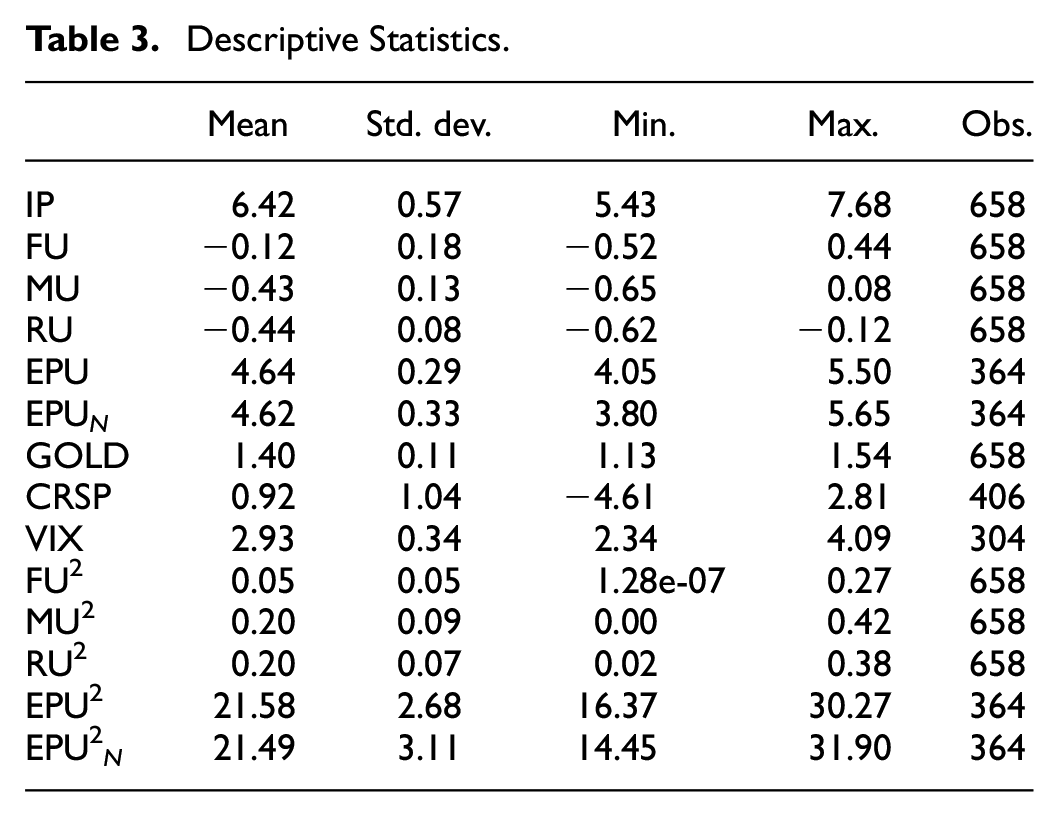
We present the descriptive statistics of our study’s variables in Table 3. According to the table, economic policy uncertainty (EPU), economic policy uncertainty news-based (EPU_N), and their quadratic terms had the highest average performance compared to other uncertainty measures. The average growth rate for economic policy uncertainty (EPU) was 4.64% with a standard deviation of 0.29%, while the average growth rate for economic policy uncertainty news-based was 4.62% with a standard deviation of 0.33%. Given the nature of the other uncertainty measures, as estimated statistically through a stochastic volatility process, all the average values are negative. The average negative growth rates for macroeconomic uncertainty, financial uncertainty, and real uncertainty were −0.43%, −0.12%, and −0.44%, with standard deviations of 0.13%, 0.18%, and 0.08%, respectively. Although there is inconsistency in the measures of uncertainty, our data indicates that industrial production has experienced a substantial growth rate despite highly volatile macroeconomic, financial, and economic policy scenarios.

Table 3.

Descriptive Statistics.

	Mean	Std. dev.	Min.	Max.	Obs.
IP	6.42	0.57	5.43	7.68	658
FU	−0.12	0.18	−0.52	0.44	658
MU	−0.43	0.13	−0.65	0.08	658
RU	−0.44	0.08	−0.62	−0.12	658
EPU	4.64	0.29	4.05	5.50	364
EPU_N	4.62	0.33	3.80	5.65	364
GOLD	1.40	0.11	1.13	1.54	658
CRSP	0.92	1.04	−4.61	2.81	406
VIX	2.93	0.34	2.34	4.09	304
FU²	0.05	0.05	1.28e-07	0.27	658
MU²	0.20	0.09	0.00	0.42	658
RU²	0.20	0.07	0.02	0.38	658
EPU²	21.58	2.68	16.37	30.27	364
EPU²_N	21.49	3.11	14.45	31.90	364

Unit Root Tests

Table 4 illustrates the results of our unit root tests to confirm the stationarity status of our selected variables. Specifically, the table reports the tests of Phillips and Perron (PP) by Phillips and Perron (1988), Augmented Dickey-Fuller (ADF) test by Dickey and Fuller (1979) and Portmanteau white noise test (WNTESTQ) by Ljung and Box (1978). Our evidence suggests that at levels I(0), the null hypothesis that the selected series are not stationary is rejected at 1% significance levels.

Table 4.

Unit Root Tests.

	ADF	ADF	PP	PP	WNTESTQ
Variables	Levels	First Difference	Levels	First Difference	Levels
IP	−1.113	−21.59***	−1.25	−21.50***	18,004.62***
FU	−2.05	−13.53***	−3.53***	−13.57***	5,318.83***
MU	−1.94	−12.83***	−3.06**	−12.51***	7,616.84***
RU	−3.53***	−16.35***	−4.53***	−15.70***	4,899.29***
EPU	−5.38***	−22.72***	−4.88***	−24.71***	2,626.04***
EPU_N	−7.60***	−23.68***	−7.44***	−26.44***	1,030.36***
GOLD	−4.32***	−17.67***	−2.96***	−18.82***	20,785.69***
CRSP	−14.55***	−24.65***	−14.80***	28.32***	2,617.41***
VIX	−4.67***	−20.30***	−4.28***	−21.64***	1,984.02***
FU²	−2.70**	−16.59***	−4.01***	−16.73***	8,736.38***
MU²	−2.03	−13.72***	−2.99***	−13.22***	8,736.38***
RU²	−3.32**	−16.18***	−4.30***	−15.56***	5,651.94***
EPU²	−5.39***	−22.57***	−4.90***	−24.56***	2,625.54***
EPU²_N	−7.60***	−23.49***	−7.45***	−26.13***	1,041.50***

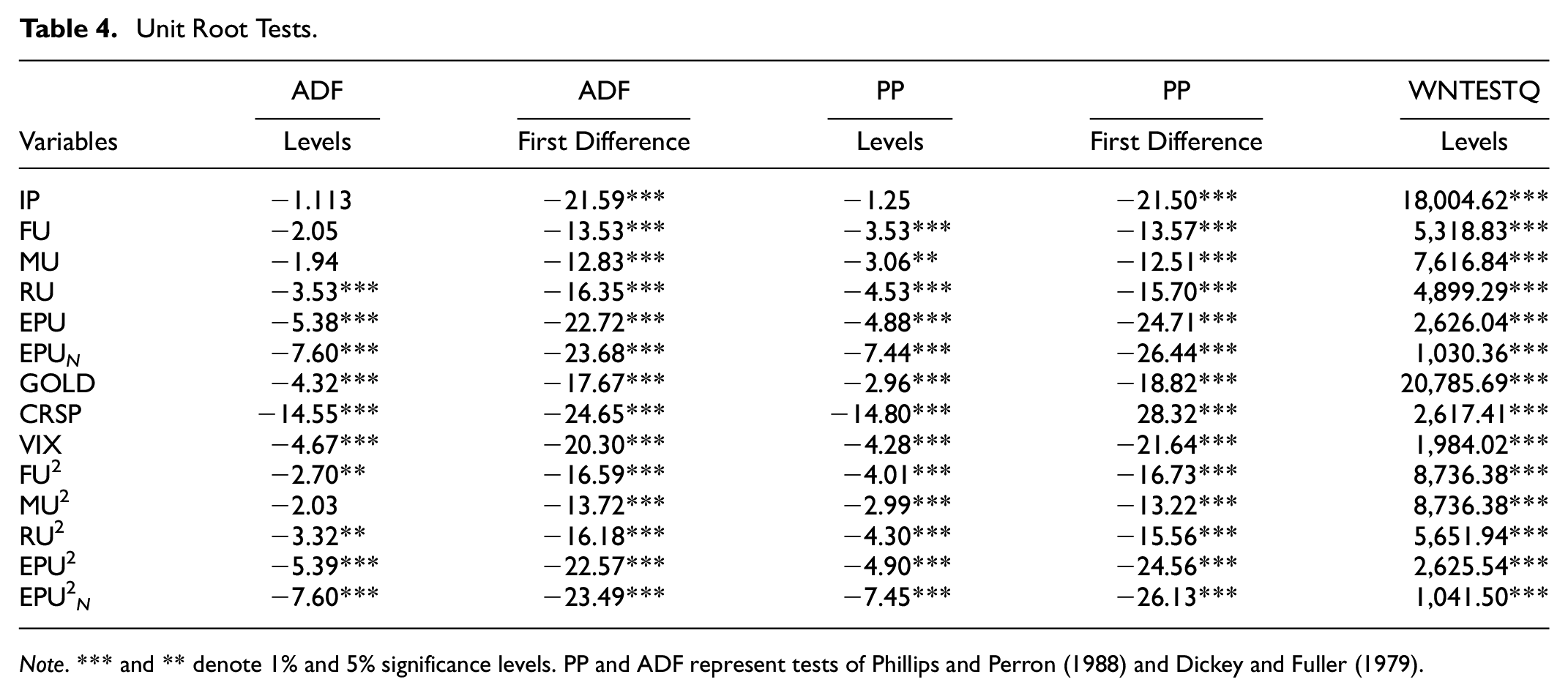
Note. *** and ** denote 1% and 5% significance levels. PP and ADF represent tests of Phillips and Perron (1988) and Dickey and Fuller (1979).

Correlations and Multicollinearity Tests

Table 5 illustrates correlations between the series. We find that the majority of the variables selected do not have significant correlations with industrial production (IP). Notably, macroeconomic uncertainty (MU), economic policy uncertainty (EPU), economic policy uncertainty news based (EPU_N), quadratic terms, and gold commodity prices (GOLD) exhibited significant correlations with industrial production. However, the quadratic term of macroeconomic uncertainty (MU²) demonstrated negative correlations with industrial production, whereas the other terms demonstrated positive correlations. We conclude that not all independent variables exhibited significant correlations with industrial production. Therefore, we contend that the date series adequately captures all the relevant data information required for long-term estimations.

Table 5.

Correlations.

	IP	FU	MU	RU	EPU	EPU_N	GOLD	CRSP	VIX	FU²	MU²	RU²	EPU²	EPU²_N
IP	1.00
FU	.04	1.00
MU	.45***	.57***
RU	−.02	.43***	.66***	1.00
EPU	.51***	.38***	.33***	.28***	1.00
EPU_N	.29***	.42***	.29***	.28***	.89***	1.00
GOLD	.58***	.03	.22***	−.35***	−.10**	.06	1.00
CRSP	.06	.30***	.14**	.07	.09	.07	.04	1.00
VIX	−.07	.87***	.54***	.46***	.42***	.49***	.14**	.30***	1.00
FU²	−.02	−.64***	−.26***	−.15***	−.28***	−.26***	.07*	−.23***	−.55***	1.00
MU²	−.45***	−.58***	−.97***	−.61***	−.31***	−.26***	−.27***	−.13**	−.50***	.35***	1.00
RU²	.05	−.42***	−.64***	−.99***	−.27***	−.26***	.37***	−.06	−.43***	.18***	.60***	1.00
EPU²	.51***	.38***	.33***	.28***	.99***	.89***	−.09*	.09	.43***	−.27***	−.31***	−.27***	1.00
EPU²_N	.29***	.42***	.30***	.28***	.89***	.99***	.06	.07	.49***	−.25***	−.26***	−.27***	.89***	1.00

Note. *** and ** denote 1% and 5% significance levels.

Furthermore, we perform a variance inflation factor analysis to reveal the tolerance of the variables in the proposed model. In this regard, we are better able to comprehend the reliability and validity of our models for the long-run estimations. We present the results in Table A1. According to the results, all the variables had tolerance levels greater than 0.20 and VIF values less than 5, indicating no evidence of multicollinearity.

Baseline Results

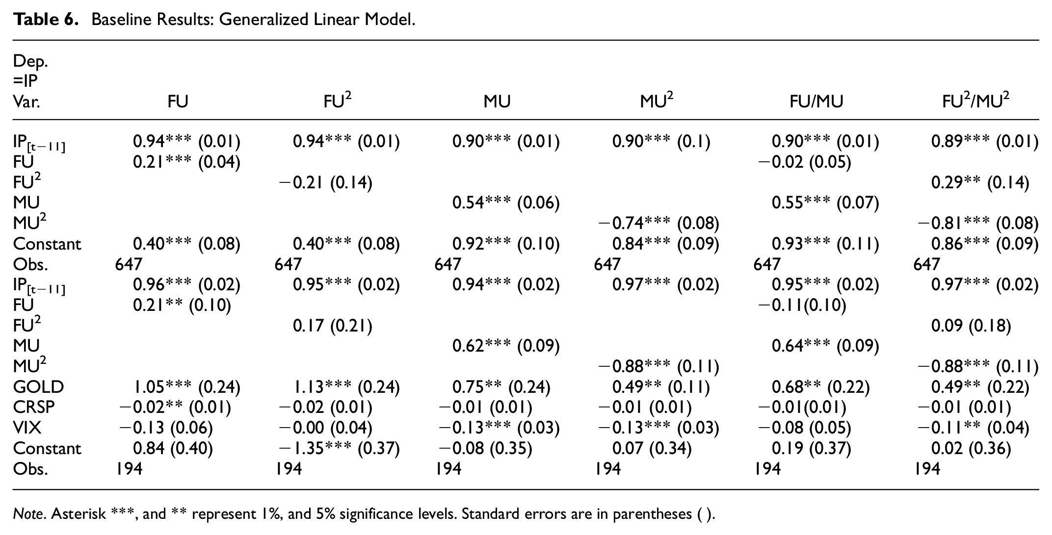
We begin our analysis by examining baseline models. Separate episodes were modeled for financial uncertainty (FU), macroeconomic uncertainty (MU), and their quadratic terms (FU² and MU²) in the baseline models. First, we model the direct impact of financial uncertainty (FU) on industrial production, then the quadratic term impact of financial uncertainty (FU²) on industrial production (IP), macroeconomic uncertainty (MU), and its quadratic term impact on industrial production (MU²) on industrial production (IP). The fifth and sixth models include both financial and macroeconomic economic uncertainties (FU and MU) as well as their quadratic terms (FU² and MU², respectively). Table 6 displays the results. The quadratic terms of financial and macroeconomic uncertainty (FU² and MU²) measure heightened levels of uncertainty, whereas the linear terms (FU and MU) measure only low levels of uncertainty.

Table 6.

Baseline Results: Generalized Linear Model.

Dep.=IPVar.	FU	FU²	MU	MU²	FU/MU	FU²/MU²
IP_[t−11]	0.94*** (0.01)	0.94*** (0.01)	0.90*** (0.01)	0.90*** (0.1)	0.90*** (0.01)	0.89*** (0.01)
FU	0.21*** (0.04)				−0.02 (0.05)
FU²		−0.21 (0.14)				0.29** (0.14)
MU			0.54*** (0.06)		0.55*** (0.07)
MU²				−0.74*** (0.08)		−0.81*** (0.08)
Constant	0.40*** (0.08)	0.40*** (0.08)	0.92*** (0.10)	0.84*** (0.09)	0.93*** (0.11)	0.86*** (0.09)
Obs.	647	647	647	647	647	647
IP_[t−11]	0.96*** (0.02)	0.95*** (0.02)	0.94*** (0.02)	0.97*** (0.02)	0.95*** (0.02)	0.97*** (0.02)
FU	0.21** (0.10)				−0.11(0.10)
FU²		0.17 (0.21)				0.09 (0.18)
MU			0.62*** (0.09)		0.64*** (0.09)
MU²				−0.88*** (0.11)		−0.88*** (0.11)
GOLD	1.05*** (0.24)	1.13*** (0.24)	0.75** (0.24)	0.49** (0.11)	0.68** (0.22)	0.49** (0.22)
CRSP	−0.02** (0.01)	−0.02 (0.01)	−0.01 (0.01)	−0.01 (0.01)	−0.01(0.01)	−0.01 (0.01)
VIX	−0.13 (0.06)	−0.00 (0.04)	−0.13*** (0.03)	−0.13*** (0.03)	−0.08 (0.05)	−0.11** (0.04)
Constant	0.84 (0.40)	−1.35*** (0.37)	−0.08 (0.35)	0.07 (0.34)	0.19 (0.37)	0.02 (0.36)
Obs.	194	194	194	194	194	194

Note. Asterisk ***, and ** represent 1%, and 5% significance levels. Standard errors are in parentheses ( ).

According to our findings presented in Table 6, in times of low levels of uncertainty, both financial and macroeconomic indicators promote industrial production, implying that lower levels of uncertainty significantly and qualitatively induce positive business cycles. In contrast, higher levels of uncertainty are detrimental to industrial production, indicating that both elevated financial and macroeconomic uncertainties impede business cycles. In addition, we introduce some variables to control the relationship between financial and macroeconomic uncertainty and industrial production. We include gold commodity prices (GOLD), economic volatility (VIX), and stock market returns (CRSP) in this context. The inclusion of the control variables has no effect on our findings. Specifically, we continue to find that low levels of financial and macroeconomic uncertainty have a substantial positive effect on industrial production, whereas high levels of macroeconomic uncertainty have a negative effect on industrial production, and high levels of financial uncertainty have no significant relationship with industrial production to deal with endogeneity or reversal causality. In all analyses, 11 lags in industrial production are included. Based on Bayesian Information Criteria, this was deemed the optimal level. The generalized linear model (GLM) performs the estimation using the identity link approach.

Robustness/Extension

Here, a Bayesian GLM robust check analysis is conducted. Incorporating prior information on the series into the Bayesian analysis is possible by assuming that all model parameters are random variables. This assumption contrasts distinctly with the GLM. We were better able to capture the dynamics of the data series and interpret the results by comparing these two empirical methods. Table 7 displays the results of our investigation. We conducted the estimations using credibility intervals of 95%. Similarly, we use the baseline models from Table 6 for the GLM analyses.

Table 7.

Robustness: Bayesian Generalized Linear Model.

Dep.Var.=IP	FU	FU²	MU	MU²	FU/MU	FU²/MU²
IP_[t−11]	0.95 (0.01)	0.94 (0.01)	0.90 (0.01)	0.90 (0.01)	0.90 (0.01)	0.89 (0.01)
FU	[0.92, 0.97]0.21 (0.04)	[0.94, 0.97]	[0.87, 0.92]	[0.87, 0.92]	[0.87, 0.92]−0.02 (0.05)	[0.86, 0.92]
FU²	[0.13, 0.30]	−0.21 (0.14)			[−0.11, 0.08]	0.29 (0.13)
MU		[−0.47, 0.05]	0.54 (0.06)		0.55 (0.07)	[0.02, 0.56]
MU²			[0.43, 0.66]	−0.74 (0.08)[−0.91,−0.59]	[0.40, 0.69]	−0.81 (0.08)[−0.97,−0.65]
Constant	0.40 (0.08)	0.40 (0.08)	0.92 (0.10)	0.83 (0.09)	0.93 (0.11)	0.87 (0.10)
Obs.	647	647	647	647	647	647
IP_[t−11]	0.95 (0.02)	0.95 (0.02)	0.95 (0.02)	0.96 (0.02)	0.95 (0.02)	0.97 (0.02)
FU	[0.91, 0.99]0.20 (0.10)	[0.92, 0.99]	[0.92, 0.99]	[0.93, 0.99]	[0.92, 0.99]−0.11 (0.10)	[0.93, 1.00]
FU²	[0.01, 0.40]	0.16 (0.20)			[−0.30, 0.08]	0.08 (0.19)
MU		[−0.23, 0.56]	0.59 (0.08)		0.64 (0.09)	[−0.23, 0.52]
MU²			[0.42, 0.73]	−0.89 (0.10)	[0.46, 0.83]	−0.89 (0.11)
GOLD	1.11 (0.23)	1.15 (0.20)	0.66 (0.23)	[−1.09,−0.68]0.49 (0.21)	0.67 (0.21)	[−1.11,−0.65]0.45 (0.23)
CRSP	[0.68, 1.61]−0.02 (0.01)	[0.67, 1.60]−0.02 (0.01)	[0.20, 1.11]−0.01 (0.01)	[0.09, 0.89]−0.01 (0.01)	[0.25, 1.09]−0.01 (0.01)	[−0.01, 0.88]−0.01 (0.01)
VIX	[−0.04,−0.00]−0.13 (0.06)	[−0.03, 0.00]−0.01 (0.041)	[−0.03, 0.01]−0.12 (0.03)	[−0.03, 0.01]−0.13 (0.03)	[−0.02, 0.01]−0.08 (0.05)	[−0.03, 0.01]−0.18 (0.04)
Constant	[−0.25,−0.02]0.90 (0.38)	[−0.08, 0.07]−1.36 (0.35)	[−0.18,−0.06]−0.05 (−0.77)	[−0.18,−0.07]0.08 (0.32)	[−0.18, 0.03]−0.19 (0.35)	[−0.19,−0.04]0.09 (0.38)
Obs.	194	194	194	194	194	194

Note. Standard deviations are in parentheses ( ) and 95% credibility intervals are in square brackets [ ].

Intriguingly, the results of the Bayesian GLM are identical to what we observed from the GLM estimations. We found that when levels of uncertainty are low, financial and macroeconomic indicators promote industrial production strongly.

Within the credibility intervals of 95% for each model, it is evident that low levels of financial and macroeconomic uncertainty are crucial for business cycles and proportionally promote industrial production. Similarly, we find that high levels of macroeconomic uncertainty worsen industrial production, which is likely to impede business cycles, whereas high levels of financial uncertainty have no effect on industrial production given that all posterior means fall within 95% confidence intervals. Even with the inclusion of control variables such as gold prices, economic volatility, and stock market returns, we still find that low levels of financial and macroeconomic uncertainty have an important effect on industrial production, whereas high levels of macroeconomic uncertainty have a negative effect on industrial production due to their negative impact on business cycles, but high levels of financial uncertainty do not matter for industrial production.

Following Ludvigson et al. (2021), we introduce additional measures of uncertainty, including real uncertainty, economic policy uncertainty, and news-based economic policy uncertainty. We present the results in Tables 8 and 9. In the same manner as the baseline models, we replace the financial and macroeconomic uncertainties with economic policy uncertainty, news-based economic policy uncertainty (EPU, EPU_N, and RU), and real uncertainty, as well as their quadratic terms (EPU², EPU²_N, and RU²). We intend to evaluate the impact of low and high levels of economic policy uncertainty, news-based economic policy uncertainty, and real uncertainty on industrial production. Our estimations were carried out using the Bayesian GLM as opposed to the GLM. This is because we are interested in the reliability of our findings. We deem it appropriate to employ the Bayesian GLM due to its statistical strength in capturing prior information and its application of the Bayes rule for performing estimations.

Table 8.

Bayesian GLM: Economic Policy Uncertainty Index Measures.

Dep.Var.=IP	EPU	EPU²	EPU_N		EPU/EPU_N	EPU²/EPU²_N
IP_[t−11]	0.93 (0.02)	0.93 (0.02)	0.96 (0.02)	0.96 (0.00)	0.89 (0.02)	0.89 (0.02)
EPU	[0.89, 0.97]0.13 (0.03)	[0.89, 0.96]	[0.93, 0.99]	[0.93, 0.99]	[0.85,0.93]0.40 (0.06)	[0.85, 0.93]
EPU²	[0.08,0.19]	0.01 (0.00)			[0.28, 0.52]	0.04 (0.01)
EPU_N		[0.01, 0.02]	0.05 (0.02)		−0.23 (0.04)	[0.03, 0.06]
EPU²_N			[0.01, 0.10]	0.01 (0.00)	[−0.33,−0.14]	−0.03 (0.01)
Constant	−0.14 (0.13)	0.17 (0.11)	0.04 (0.13)	[0.00,0.01]0.15 (0.11)	−0.05 (0.10)	[−0.04,−0.01]0.33 (0.11)
Obs.	364	364	364	364	364	364
IP_[t−11]	0.87 (0.02)	0.87 (0.02)	0.95 (0.02)	0.95 (0.02)	0.82 (0.02)	0.82 (0.02)
EPU	[0.83, 0.92]0.19 (0.04)	[0.82, 0.91]	[0.90, 0.99]	[0.90, 0.99]	[0.78, 0.86]0.69 (0.07)	[0.77, 0.86]
EPU²	[0.12, 0.26]	0.02 (0.00)			[0.55, 0.83]	0.08 (0.01)
EPU_N		[0.01, 0.03]	0.02 (0.03)		−0.46 (0.06)	[0.06,0.09]
EPU²_N			[−0.04,0.08]	0.00 (0.00)	[−0.57,−0.34]	−0.05 (0.01)
GOLD	1.43 (0.23)	1.61 (0.16)	1.17 (0.25)	[−0.00, 0.01]1.13 (0.12)	1.65 (0.11)	[−0.06,−0.04]1.61 (0.19)
CRSP	[0.98, 1.89]−0.12 (0.01)	[1.31, 1.91]−0.01 (0.01)	[0.70, 1.66]−0.01 (0.01)	[0.91, 1.37]−0.02 (0.01)	[1.46, 1.83]−0.01 (0.01)	[1.25, 2.01]−0.01 (0.01)
VIX	[−0.30,0.01]−0.11 (0.03)	[−0.03,0.01]−0.12 (0.03)	[−0.03,0.00]−0.04 (0.04)	[−0.03, 0.01]−0.03 (0.04)	[−0.03,0.01]−0.10 (0.03)	[−0.03,0.01]−0.10 (0.03)
Constant	[−0.18,−0.05]−1.84 (0.33)	[−0.18,−0.06]−1.58 (0.27)	[−2.02,−0.65]−1.35 (0.35)	[−0.10,0.04]−1.24 (0.19)	[−0.16,−0.05]−2.02 (0.14)	[−0.16,−0.04]−1.43 (0.26)
	194	194	194	194	194	194

Note. Standard deviations are in parentheses ( ) and 95% credibility intervals are in square brackets [ ].

Table 9.

Extension: Bayesian Generalized Linear Model Real Uncertainty Measures.

Dep. Var. = IP	RU	RU²
IP_[t−11]	0.94 (0.01)	0.95 (0.01)
RU	[0.92,0.97]0.47 (0.09)	[0.92, 0.97]
RU²	[0.31, 0.63]	−0.56 (0.10)
Constant Obs.	0.56(0.09) 647	[−0.76, −0.36]0.46 (0.08)647
IP_[t−11]	0.93 (0.02)	0.94 (0.02)
RU	[0.90,0.97]0.63 (0.14)	[0.90, 0.97]
RU²	[0.38, 0.89]	−0.77 (0.14)
GOLD	1.00 (0.23)	[−1.05, −0.53]0.84 (0.14)
CRSP	[0.38, 0.90]−0.01 (0.01)	[0.57, 1.09]−0.01 (0.01)
VIX	[−0.03, 0.01]−0.08 (0.03)	[−0.03, 0.00]−0.08 (0.03)
Constant	[−0.14, −0.02]−0.49 (0.03)	[−0.14, −0.02]−0.40 (0.19)
Obs.	194	194

Note. Standard deviations are in parentheses ( ) and 95% credibility intervals are in square brackets [ ].

In Table 8, the impact of low and high levels of economic policy uncertainty and economic policy uncertainty-based news on industrial production is presented. Our findings indicate that both low and high levels of economic policy uncertainty considerably raise industrial production. This implies that economic policy uncertainty has an important effect on industrial production even during times of higher levels of uncertainty. According to economic policy uncertainty reported in the news, there are low and high levels of uncertainty worsen industrial production, whereas low levels of uncertainty promote industrial production given that all posterior means fall within 95% confidence intervals. In Table 9, we present the real uncertainty’s effect on industrial production. Our findings indicate that low levels of uncertainty are advantageous and essential for industrial production, while high levels of uncertainty are detrimental, given that all posterior means fall within 95% confidence intervals. Even after adjusting for gold prices (GOLD), economic volatility (VIX), and stock market returns (CRSP), the significance of these findings remains.

After this, we test for Granger causality between important variables such as financial uncertainty, macroeconomic uncertainty, the quadratic terms of financial and macroeconomic uncertainties, and industrial production. The test results are presented in Table 10. Our evidence suggests that macroeconomic uncertainty and its quadratic term cause industrial production, while financial uncertainty causes macroeconomic uncertainty. Alternatively, we observe a bidirectional Granger causality between the quadratic term of macroeconomic uncertainty and financial uncertainty. This implies that low levels of financial uncertainty are likely to lead to low levels of macroeconomic uncertainty, but in an environment of elevated macroeconomic uncertainty, macroeconomic indicators cause a significant decline in industrial production. In addition, high financial uncertainty causes high macroeconomic uncertainty, whereas high macroeconomic uncertainty also causes high financial uncertainty. In contrast, the effect of high levels of macroeconomic uncertainty on high levels of financial uncertainty is contemporaneous, whereas the response of macroeconomic uncertainty to high levels of financial uncertainty takes over 60 months. There is strong evidence that the causality test and the long-run estimates are consistent. This suggests that macroeconomic uncertainty is more important than financial uncertainty when it comes to industrial production. However, financial uncertainty makes macroeconomic uncertainty much worse, which in turn makes industrial production much worse, which causes business cycles to change.

Table 10.

Granger Causality Test.

Causality	Lags	T-stats. (p-value)	Remarks
MU → FU FU → MU	66	7.89 (.25)18.69*** (.00)	No causalityUnidirectional causality
FU → MUMU²→ FU²	601	81.00 (.04)3.89 (.05)	BirectionalBirectional
MU → IPIP → qMU	11	3.77** (.06)11.04 (.44)	Unidirectional causalityNo causality
MU → IPIP → MU²	11	4.97** (.03)12.04 (.48)	Unidirectional causalityNo causality
FU → IPIP → FU	44	8.27 (.08)4.16 (.30)	No causalityNo causality
FU → IPIP → FU²	1111	5.21 (.92)12.78 (.31)	No causalityNo causality

To ensure comprehensiveness, we conducted a regression analysis using Newey-West standard errors. We employed this approach to address potential endogeneity issues that could arise from autocorrelation between the error terms and the dependent variable (Newey & West, 1987). The regression model is estimated using the Ordinary Least Squares (OLS) method, and the p-values are adjusted for heteroskedasticity and autocorrelation up to 11 lags using the Newey and West (1987) standard errors, which are known for their robustness. The findings are displayed in Table A2 located in the Appendix. The results indicate that the coefficients and p-values obtained from the generalized linear model (GLM) and Bayesian GLM estimations are equivalent to those obtained from the Newey-West standard errors regression once autocorrelation and heteroskedasticity have been accounted for. The presented evidence suggests that our findings are valid, and it is plausible that endogeneity issues did not affect our respective models.

Discussion

We find strong evidence that macroeconomic uncertainty, as opposed to financial uncertainty, has the greatest impact on business cycles when economic uncertainty is elevated. Similarly, we find that both news-based and real economic policy uncertainty significantly worsen industrial production, indicating a downward trend in business cycles or the likelihood of a recession. According to Baker et al. (2016), when policy uncertainty increases, businesses that are more exposed to government spending slow down employment and investment growth. This finding suggests that the EPU indices are effective indicators of real economic uncertainty. A strand of literature in support of this argument emphasized that high levels of uncertainty cause financial constraints and perhaps are likely to hamper precautionary savings since the adverse effects of uncertainty result to real options; see Bernanke (1983), McDonald and Siegel (1986), Gilchrist et al. (2014), and Basu and Bundick (2017). According to the findings of Bloom et al. (2018), heightened levels of uncertainty have the potential to diminish the short-term effectiveness of first-moment policies, such as wage subsidies. Firms tend to exercise greater caution in their responses to fluctuations in prices, which contributes to this effect.

High levels of macroeconomic uncertainty are presumably characterized by risky behavior, which leads to a larger misallocation of capital across sectors. This is likely to generate a countercyclical uncertainty effect in consumption growth as a result of irreversible and expensive investments (Bachmann et al., 2013; Fajgelbaum et al., 2017; Pástor & Veronesi, 2013). Bernanke (1983) suggests that an increase in economic uncertainty reduces total demand in the economy via a conventional channel that is associated with real option theory. In times of high uncertainty, businesses and, in the case of durable goods, consumers are more likely to exercise extreme caution to avoid the substantial financial losses associated with making poor investment decisions. Consequently, decisions regarding investments, employment, and expenditures are postponed until there is less uncertainty; see Bloom (2009), Baker et al. (2016), and Bloom et al. (2018).

In contrast to Ludvigson et al. (2021), we find that low levels of financial uncertainty contribute positively to industrial production or real economic activity characterized by stable and progressive business cycles. Despite the negative impact of financial uncertainty on industrial output, Ghosh et al. (2021) contend that the relationship is quite insignificant. This suggests that high levels of financial uncertainty do not contribute significantly to industrial production.

Conclusion

In accordance with increasing evidence from research, deep recessions are characterized by uncertainty, but two crucial questions remain unanswered: Is uncertainty the primary cause of changes in the business cycle? Does it matter which type of uncertainty exists? The purpose of this study is to econometrically address both questions using generalized linear models and Bayesian generalized linear models, which can capture the non-normal distribution of the errors in the data series. We assess the situation of the US economy from 1960 to 2015 using monthly data sourced from Ludvigson et al. (2021).

Most of the macro-literature on uncertainty has focused on macro-uncertainty caused by real activity as a source of economic fluctuations. Based on numerous estimations employing diverse measures of uncertainty. We have come to the conclusion that high levels of macroeconomic uncertainty, which is comparable to real uncertainty, exhibit counter-cyclical behavior with respect to business cycles as well as economic policy uncertainty as measured by news. Business cycles respond favorably to low levels of uncertainty, which supports an increase in industrial production, but negatively to high levels of uncertainty, resulting in decreased industrial output. We find strong evidence of consistency between the causality test and the long-run estimations, indicating that macroeconomic uncertainty matters more than financial uncertainty in relation to industrial production, but financial uncertainty causes macroeconomic uncertainty to significantly exacerbate industrial production, thereby causing business cycle fluctuations. This observation strongly indicates the presence of an inverted U-shaped relationship between macroeconomic uncertainty and business cycles, while a linear relationship is observed between financial uncertainty and industrial production.

Contrary to the findings of Ludvigson et al. (2021), we conclude that high levels of macroeconomic uncertainty matter more than financial uncertainty, despite our findings indicating that low levels of financial and macroeconomic uncertainties are significant and positive drivers of industrial production. High levels of macroeconomic uncertainty have a ripple effect on the entire economy, stifling investments, reducing consumption, and creating unemployment, which is likely to have an effect on labor participation.

Policy Implication

Elevated levels of uncertainty possess the potential to disrupt the natural progression of business cycles and consequently diminish industrial production. In light of this, policy- makers may find it necessary to adopt appropriate measures aimed at alleviating uncertainty in times of economic downturns. The results indicate that in periods of economic contraction, the reduction of macroeconomic uncertainty can serve as a viable strategy for mitigating fluctuations in business cycles and enhancing levels of industrial production. When formulating monetary policy and determining interest rates, central banks and monetary policymakers should consider the influence of macroeconomic uncertainty. Increased levels of uncertainty can potentially lead to a more accommodating approach to facilitate the process of economic recovery. The results of this study could potentially have significant ramifications for the realm of international trade and the dynamics of global economic interactions.

The presence of significant macroeconomic uncertainty has the potential to exert an impact on various aspects of the global economy, including supply chains, trade patterns, and decisions pertaining to foreign direct investment. The presence of elevated levels of macroeconomic uncertainty can potentially result in a decrease in research and development (R&D) expenditures by firms, as they may exhibit a heightened aversion to risk. The phenomenon may potentially yield significant consequences for the advancement of innovation and the maintenance of industrial competitiveness in the long run. Elevated levels of macroeconomic uncertainty have the potential to engender heightened levels of volatility within financial markets, thereby exerting an influence on the valuation of assets, the determination of interest rates, and the direction of capital flows. The phenomenon may potentially result in repercussions that extend beyond national borders, thereby impacting the overall stability of the global financial system.

Limitation and Future Research Direction

We acknowledge that the study may have some limitations given that it does not account for the potential influence of external shocks or events, such as the COVID-19 pandemic, natural disasters, geopolitical events, or major technological disruptions, which can have a substantial effect on industrial production. During the analysis conducted in this study, there were substantial transformations in the global economic landscape and financial markets over multiple decades. Shifts in economic policies, financial regulations, and the process of globalization may have influenced the relationship between uncertainty and industrial production.

To get around these problems, researchers need to use accurate and up-to-date data sources, think about different model specifications, do thorough robustness checks, and be aware of the possibility of endogeneity and missing variables. Furthermore, it is imperative to exercise caution and consider the specific data and methodologies employed when interpreting the findings of the study.

Footnotes

Appendix

Declaration of Conflicting Interests

The author(s) declared no potential conflicts of interest with respect to the research, authorship, and/or publication of this article.

Funding

The author(s) received no financial support for the research, authorship, and/or publication of this article.

ORCID iDs

Prince Asare Vitenu-Sackey

Isaac Akpemah Bathuure

Data Availability Statement

The data used in this study has been stored in Mendeley Data with DOI: Will be provided after reviewing due to anonymity policy.

References

Abel

A. B.

(1983). Optimal investment under uncertainty. American Economic Review, 73(1), 228–233.

Afonso

Blanco-Arana

M. C.

(2022). Financial and economic development in the context of the global 2008-09 financial crisis. International Economics, 169, 30–42.

Ajayi

Aliyev

Sarkhanov

(2020). The Impact of Covid-19 Coronavirus on Financial Markets: A Qualitative Approach [Conference session]. In Economic and Social Development (Book of Proceedings Vol. 1/4), 55th International Scientific Conference on Economic and Social, volume 59, p. 567.

Ali

Hongbing

Liew

C. Y.

Jianguo

(2023). Governance perspective and the effect of economic policy uncertainty on financial stability: Evidence from developed and developing economies. Economic Change and Restructuring, 56(3), 1971–2002.

Al-Thaqeb

S. A.

Algharabali

B. G.

(2019). Economic policy uncertainty: A literature review. Journal of Economic Asymmetries, 20, e00133.

Arellano

Bai

Kehoe

(2010). Financial markets and fluctuations in uncertainty. Federal Reserve Bank of Minneapolis Working Paper.

Bachmann

Elstner

Sims

E. R.

(2013). Uncertainty and economic activity: Evidence from business survey data. American Economic Journal Macroeconomics, 5(2), 217–249.

Baker

S. R.

Bloom

Davis

S. J.

(2016). Measuring economic policy uncertainty. Quarterly Journal of Economics, 131(4), 1593–1636.

Baker

S. R.

Bloom

Terry

S. J.

(2020). Using disasters to estimate the impact of uncertainty. Technical report, National Bureau of Economic Research.

10.

Bar-Ilan

Strange

W. C.

(1996). Investment lags. The American Economic Review, 86(3), 610–622.

11.

Basu

Bundick

(2017). Uncertainty shocks in a model of effective demand. Econometrica, 85(3), 937–958.

12.

Belsley

D. A.

Kuh

Welsch

R. E.

(2005). Regression diagnostics: Identifying influential data and sources of collinearity. John Wiley & Sons.

13.

Bernanke

B. S.

(1983). Irreversibility, uncertainty, and cyclical investment. Quarterly Journal of Economics, 98(1), 85–106.

14.

BlLLINGS

S. A.

Voon

W. S. F.

(1986). Correlation based model validity tests for non-linear models. International Journal of Control, 44(1), 235–244.

15.

Bloom

(2009). The impact of uncertainty shocks. Econometrica, 77(3), 623–685.

16.

Bloom

Floetotto

Jaimovich

Saporta-Eksten

Terry

S. J.

(2018). Really uncertain business cycles. Econometrica, 86(3), 1031–1065.

17.

Blough

D. K.

Madden

C. W.

Hornbrook

M. C.

(1999). Modeling risk using generalized linear models. Journal of Health Economics, 18(2), 153–171.

18.

Bollerslev

Tauchen

Zhou

(2009). Expected stock returns and variance risk premia. Review of Financial Studies, 22(11), 4463–4492.

19.

Bonciani

Ricci

(2020). The international effects of global financial uncertainty shocks. Journal of International Money and Finance, 109, 102236.

20.

Born

Breuer

Elstner

(2018). Uncertainty and the great recession. Oxford Bulletin of Economics and Statistics, 80(5), 951–971.

21.

Born

Pfeifer

(2021). Uncertainty-driven business cycles: Assessing the markup channel. Quantitative Economics, 12(2), 587–623.

22.

Broock

W. A.

Scheinkman

J. A.

Dechert

W. D.

LeBaron

(1996). A test for independence based on the correlation dimension. Econometric Reviews, 15(3), 197–235.

23.

Carriere-Swallow

M. Y.

Magud

M. N. E.

Werner

A. M.

(2016). Central banking in Latin America: The way forward. International Monetary Fund.

24.

Cascaldi-Garcia

Sarisoy

Londono

J. M.

Rogers

J. H.

Datta

Ferreira

Grishchenko

Jahan-Parvar

O. V.

Loria

M. R.

F., S.

, (2023). What is certain about uncertainty? Journal of Economic Literature, 61(2), 624–654.

25.

Cerra

Fatás

Saxena

S. C.

(2023). Hysteresis and business cycles. Journal of Economic Literature, 61(1), 181–225.

26.

Chen

Rahaman

M. A.

Hossain

M. A.

Chen

(2023). Is growth of the financial sector relevant for mitigating CO2 emissions in Bangladesh? The moderation role of the financial sector within the EKC model. Environment Development and Sustainability, 25(9), 9567–9588.

27.

Chetty

Friedman

J. N.

Hendren

Stepner

; & The Opportunity Insights Team. (2020). How did COVID-19 and stabilization policies affect spending and employment? A new real-time economic tracker based on private sector data (Vol. 91, pp. 1689–1699). National Bureau of Economic Research.

28.

Choudhry

Hassan

S. S.

Shabi

(2020a). US economic uncertainty, EU business cycles, and the global financial crisis. International Journal of Finance & Economics, 25(1), 28–42.

29.

Chowdhury

M. A. F.

Meo

M. S.

Aloui

(2021). How world uncertainties and global pandemics destabilized food, energy and stock markets? Fresh evidence from quantile on quantile regressions. International Review of Financial Analysis, 76, 101759.

30.

Ciarlantini

Madaleno

Robaina

Monteiro

Eusébio

Carneiro

M. J.

Gama

(2023). Air pollution and tourism growth relationship: Exploring regional dynamics in five European countries through an EKC model. Environmental Science and Pollution Research, 30(15), 42904–42922.

31.

Demir

Ersan

(2017). Economic policy uncertainty and cash holdings: Evidence from BRIC countries. Emerging Markets Review, 33, 189–200.

32.

Dew-Becker

Giglio

(2023). Cross-sectional uncertainty and the business cycle: Evidence from 40 years of options data. American Economic Journal Macroeconomics, 15(2), 65–96.

33.

Dickey

D. A.

Fuller

W. A.

(1979). Distribution of the estimators for autoregressive time series with a unit root. Journal of the American Statistical Association, 74(366a), 427–431.

34.

Diggle

(1990). Time series: A biostatistical introduction. Oxford University Press.

35.

Dreyer

Schulz

(2023). Policy uncertainty and corporate investment: Public versus private firms. Review of Managerial Science, 17(5), 1863–1898.

36.

Durbin

Watson

G. S.

(1971). Testing for serial correlation in least squares regression. III. Biometrika, 58(1), 1–19.

37.

Fajgelbaum

P. D.

Schaal

Taschereau-Dumouchel

(2017). Uncertainty traps. Quarterly Journal of Economics, 132(4), 1641–1692.

38.

Fernández-Villaverde

Guerrón-Quintana

Rubio-Ramírez

J. F.

Uribe

(2011). Risk matters: The real effects of volatility shocks. American Economic Review, 101(6), 2530–2561.

39.

Fostel

Geanakoplos

(2012). Why does bad news increase volatility and decrease leverage? Journal of Economic Theory, 147(2), 501–525.

40.

Gadzo

S. G.

Kportorgbi

H. K.

Gatsi

J. G.

(2019). Credit risk and operational risk on financial performance of universal banks in Ghana: A partial least squared structural equation model (PLS SEM) approach. Cogent Economics & Finance, 7(1), 1589406.

41.

Ganong

Noel

(2019). Consumer spending during unemployment: Positive and normative implications. American Economic Review, 109(7), 2383–2424.

42.

Ghosh

Sahu

Chattopadhyay

(2021). Inflation expectations of households in India: Role of oil prices, economic policy uncertainty, and spillover of global financial uncertainty. Bulletin of Economic Research, 73(2), 230–251.

43.

Gilchrist

Sim

J. W.

Zakrajšek

(2014). Uncertainty, financial frictions, and investment dynamics. Technical report, National Bureau of Economic Research.

44.

Gilks

W. R.

Wild

(1992). Adaptive rejection sampling for Gibbs sampling. Journal of the Royal Statistical Society Series C (Applied Statistics), 41(2), 337–348.

45.

Glaeser

E. L.

Santos

Weyl

E. G.

(2019). After the flood: how the great recession changed economic thought. University of Chicago Press.

46.

Granger

C. W. J.

(1969). Investigating causal relations by econometric models and cross-spectral methods. Econometrica, 37, 424–438.

47.

Grossman

G. M.

Krueger

A. B.

(1995). Economic growth and the environment. Quarterly Journal of Economics, 110(2), 353–377.

48.

Guerard

J. B.

Mark

(2003). The optimization of efficient portfolios: The case for an R&D quadratic term. In Research in finance (Vol 20, pp. 213–247). Emerald Group Publishing Limited.

49.

Gunst

R. F.

(1984). Comment: Toward a balanced assessment of collinearity diagnostics. American Statistician, 38(2), 79–82.

50.

Hamilton

J. D.

(1994). Time series analysis. Princeton University Press.

51.

Hartman

(1972). The effects of price and cost uncertainty on investment. Journal of Economic Theory, 5(2), 258–266.

52.

Hastie

T. J.

Pregibon

(2017). Generalized linear models. In T.J. Hastie (ed.), Statistical models in S (pp. 195–247). Routledge.

53.

Ilut

Saijo

(2021). Learning, confidence, and business cycles. Journal of Monetary Economics, 117, 354–376.

54.

Johnson

Kozicki

Priftis

Suchanek

Witmer

Yang

(2020). Implementation and effectiveness of extended monetary policy tools: Lessons from the literature (No. 2020-16). Bank of Canada Staff Discussion Paper.

55.

Junttila

Vataja

(2018). Economic policy uncertainty effects for forecasting future real economic activity. Economic Systems, 42(4), 569–583.

56.

Jurado

Ludvigson

S. C.

(2015). Measuring uncertainty. American Economic Review, 105(3), 1177–1216.

57.

Kalu

J. U.

Buang

Aliagha

G. U.

(2016). Determinants of voluntary carbon disclosure in the corporate real estate sector of Malaysia. Journal of Environmental Management, 182, 519–524.

58.

Khan

M. A.

Qin

Jebran

Rashid

(2020). The sensitivity of firms’ investment to uncertainty and cash flow: Evidence from listed state-owned enterprises and non-state-owned enterprises in China. Sage Open, 10(1), 2158244020903433.

59.

Kirschen

D. S.

Strbac

(2018). Fundamentals of power system economics. John Wiley & Sons.

60.

Kraft

Schwartz

Weiss

(2018). Growth options and firm valuation. European Financial Management, 24(2), 209–238.

61.

Lakshmi

Thenmozhi

Varaiya

(2019). Determinants of aggregate credit flows to U.S. Corporate and noncorporate sector. Sage Open, 9(1), 2158244018823082.

62.

Leduc

Liu

(2016). Uncertainty shocks are aggregate demand shocks. Journal of Monetary Economics, 82, 20–35.

63.

Leduc

Liu

(2020). The uncertainty channel of the coronavirus. FRBSF Economic Letter, 7:1–05.

64.

Lee

Daunizeau

(2020). Choosing what we like vs liking what we choose: How choice-induced preference change might actually be instrumental to decision-making. Plos One, 15(5), e0231081.

65.

Lees

White

Zhang

Ram

Gatzke-Kopp

L. M.

(2022). Decision-making in uncertain contexts: The role of autonomic markers in resolving indecision. International Journal of Psychophysiology, 177, 220–229.

66.

Lindsey

J. K.

(2000). Applying generalized linear models. Springer Science & Business Media.

67.

Zhang

Cai

T. T.

(2023). Estimation and inference for high-dimensional generalized linear models with knowledge transfer. Journal of the American Statistical Association, 1–12.

68.

Liu

(2021). U.S. Economic uncertainty shocks and China’s economic activities: A Time-varying perspective. Sage Open, 11(3), 21582440211032672.

69.

Zhong

(2020). Impact of economic policy uncertainty shocks on China’s financial conditions. Finance Research Letters, 35, 101303.

70.

Ljung

G. M.

Box

G. E. P.

(1978). On a measure of lack of fit in time series models. Biometrika, 65(2), 297–303.

71.

Ludvigson

S. C.

(2021). Uncertainty and business cycles: Exogenous Impulse or endogenous response? American Economic Journal Macroeconomics, 13(4), 369–410.

72.

McCullagh

(Ed.). (1989). Generalized linear models (2nd ed.). Routledge.

73.

McCulloch

C. E.

(2000). Generalized linear models. Journal of the American Statistical Association, 95(452), 1320–1324.

74.

McDonald

Siegel

(1986). The value of waiting to invest. Quarterly Journal of Economics, 101(4), 707–727.

75.

Myers

R. H.

Montgomery

D. C.

(1997). A tutorial on generalized linear models. Journal of Quality Technology, 29(3), 274–291.

76.

Nakamura

Sergeyev

Steinsson

(2017). Growth-rate and uncertainty shocks in consumption: Cross-country evidence. American Economic Journal Macroeconomics, 9(1), 1–39.

77.

Nelder

J. A.

Wedderburn

R. W. M.

(1972). Generalized linear models. Journal of the Royal Statistical Society. Series A, (Statistics in Society), 135(3), 370–384.

78.

Neter

Wasserman

Kutner

M. H.

(1983). Applied linear regression models. Richard D. Irwin.

79.

Neuhaus

McCulloch

(2011). Generalized linear models. Wiley Interdisciplinary Reviews Computational Statistics, 3(5), 407–413.

80.

Newey

W. K.

West

K. D.

(1987). A simple, positive semi-definite, heteroskedasticity and autocorrelation consistent covariance matrix. Econometrica, 55, 703–708.

81.

Wright

J. H.

(2013). Facts and challenges from the great recession for forecasting and macroeconomic modeling. Journal of Economic Literature, 51(4), 1120–1154.

82.

Nowzohour

Stracca

(2020). More than a feeling: Confidence, uncertainty, and macroeconomic fluctuations. Journal of Economic Surveys, 34(4), 691–726.

83.

O'connor

. (2017). The fiscal crisis of the state. Routledge.

84.

W. Y.

(1961). The desirability of price instability under perfect competition. Econometrica, 29, 58–64.

85.

Pástor, Veronesi

. (2013). Political uncertainty and risk premia. Journal of Financial Economics, 110(3), 520–545.

86.

Phillips

P. C. B.

Perron

(1988). Testing for a unit root in time series regression. Biometrika, 75(2), 335–346.

87.

Rovine

M. J.

von Eye

(1997). A 14th way to look at a correlation coefficient: Correlation as the proportion of matches. American Statistician, 51(1), 42–46.

88.

Seethaler

P. M.

Fuchs

L. S.

Fuchs

Compton

D. L.

(2012). Predicting first graders’ development of calculation versus word-problem performance: The role of dynamic assessment. Journal of Education & Psychology, 104(1), 224–234.

89.

Segal

Shaliastovich

Yaron

(2015). Good and bad uncertainty: Macroeconomic and financial market implications. Journal of Financial Economics, 117(2), 369–397.

90.

Thompson

C. G.

Kim

R. S.

Aloe

A. M.

Becker

B. J.

(2017). Extracting the variance inflation factor and other multicollinearity diagnostics from typical regression results. Basic and Applied Social Psychology, 39(2), 81–90.

91.

Trung

N. B.

(2019). The spillover effects of US economic policy uncertainty on the global economy: A global VAR approach. North American Journal of Economics and Finance, 48, 90–110.

92.

Ulucak

Bilgili

(2018). A reinvestigation of EKC model by ecological footprint measurement for high, middle and low income countries. Journal of Cleaner Production, 188, 144–157.

93.

Van Nieuwerburgh

Veldkamp

. (2006). Learning asymmetries in real business cycles. Journal of Monetary Economics, 53(4), 753–772.

94.

Vidal

(2021). Recession, financial instability, social inequality, and the health crisis. Review of Political Economy, 33(4), 711–724.

95.

Volpin

Maximiano

(2020). The Role of Competition Policy in Promoting Economic Recovery. Available at SSRN3917877.

96.

Wang

Zhang

Cui

Zhang

(2023). Role of fiscal and monetary policies for economic recovery in China. Economic Analysis and Policy, 77, 51–63.

97.

Wen

Sha

Shao

(2021). How does economic policy uncertainty affect corporate risk-taking? Evidence from China. Finance Research Letters, 41 101840.

98.

Wuthisatian

Thanetsunthorn

(2018). The Asian financial crisis: Market inefficiency and speculative bubbles. International Journal of Financial Markets and Derivatives, 6(3), 240–267.

99.

Xia

Nan

(2023). Debiased lasso for generalized linear models with a diverging number of covariates. Biometrics, 79(1), 344–357.

100.

Yang

(2017). Stock market crash, new market failure theory and extremely great economic and financial crises. World Review of Political Economy, 8(1), 4–34.

101.

Yellen

J. L.

(2015). Monetary policy and financial stability. International Monetary Fund.

102.

Yin

Chen

Kong

(2023). Empirical likelihood for generalized linear models with longitudinal data. Journal of Systems Science and Complexity, 36, 2100–2124.

103.

Zhang

Hyder

Baloch

Z. A.

Qian

Berk Saydaliev

(2022). Nexus between oil price volatility and inflation: Mediating nexus from exchange rate. Resources Policy, 79, 102977.

104.

Zhao

Wang

Zhou

(2016). Understanding the relation between urbanization and the eco-environment in China's Yangtze River delta using an improved EKC model and coupling analysis. Science of the Total Environment, 571, 862–875.

105.

Zhu

Escanciano

J. C.

(2017). Automatic portmanteau tests with applications to market risk management. The Stata Journal, 17(4), 901–915.

Uncertainty Measures and Business Cycles: Evidence From the US

Abstract

Plain Language Summary

Keywords

Introduction

Brief Literature Review

Uncertainty in the US

Empirical Methods/Data

Data Sources

Empirical Strategy

Empirical Model

Empirical Methods

Unit Root Tests

Correlations and Multicollinearity Tests

Long-Run Estimations: Generalized Linear Model

Long-Run Estimations: Bayesian Generalized Linear Model

Granger Causality Test

Empirical Results

Descriptive Statistics

Unit Root Tests

Correlations and Multicollinearity Tests

Baseline Results

Robustness/Extension

Discussion

Conclusion

Policy Implication

Limitation and Future Research Direction

Footnotes

Appendix

Declaration of Conflicting Interests

Funding

ORCID iDs

Data Availability Statement

References