Dynamic Asymmetric Causality of Bitcoin’s Price-Volume Relation

Abstract

Bitcoin has attracted incessant attentions in recent times. Studies have completed models to examine the relationship between Bitcoin and other multiple attendant variables. This paper considers a simple and direct price-volume relation. The paper offers causality evidence according to the dynamic asymmetric causality test. Based on available monthly data spanning 2010:M7-2022:M10, the paper shows that Bitcoin price and volume are integrated, both been I(0)’s. Moreover, the paper discloses the short- and long-term price-volume behaviors of Bitcoin using the cointegration test and vector error correction model (VECM). Taken together, the study first confirms long run relations and presents the estimates of the parsimonious VECM. The results show short run evidence of positive price-volume relations, and in the long run, the disequilibria are as well corrective and mean reversing. The outcomes of the Hatemi-J’s causality testing suggest likely evidence of bidirectional causality between the positive and negative fragments of the shocks of Bitcoin price and volume during the periods.

Introduction

Bitcoin, the first cryptocurrency, is created on cryptography, decentralization and openness to compete with the traditional payment systems and digital currencies. Bitcoin continues to attract incessant attentions (Urquhart, 2018), unlike when it was invented and its market considered weak and inefficient (Bouri et al., 2017; Kliber et al., 2019; Urquhart, 2016). The cryptocurrency has been investigated for different purpose. Testing of semi-strong case market efficiency shows market inefficiency (Li et al., 2021; Shen et al., 2019; Wei, 2018). Empirical tests using twitter’s tweet (Shen et al., 2019), Google search (Li et al., 2021; Gbadebo et al., 2021; Urquhart, 2018), and economic policy uncertainty (E. Demir et al., 2018) reject the market efficiency. Wei (2018) found that the predictability of Bitcoin returns is less likely relative to other cryptocurrencies, and that expected Bitcoin return likely decreases as liquidity increases. Gbadebo et al. (2021) show how Bitcoin fundamentals and Google search drive Bitcoin price swings, revealing that the market impinged greater influence than information.

Strand of studies on Bitcoin explore different aspects, including hedging and safe haven suitability of Bitcoin (Bouri et al., 2017; Dyhrberg, 2016; Kliber et al., 2019; how trading volume is associated with spillover across cryptocurrencies (Bouri et al., 2021; Ji et al., 2019); relationship between cryptocurrency return and trading volume (Alaoui et al., 2019a; Balcilar et al., 2017; Bouri et al., 2019; M. Naeem et al., 2020) as well as how cryptocurrency relates with stock returns (Lahiani et al., 2021). Kliber et al. (2019) identified that Bitcoin is a safe haven and substitute for typical financial assets. Bouri et al. (2017) revealed that Bitcoin is a weak hedge but suitable diversification tool. Dyhrberg (2016) noted that Bitcoin hedges against other financial assets, but response to news are asymmetric. Bouri et al. (2021) showed that Bitcoin return equicorrelation is very time-varying, and trading volume and uncertainties are main determinants of integration. Ji et al. (2019) showed that both Bitcoin and Litecoin exhibit strong connection of network of returns. Lahiani et al. (2021) indicated that the BSE 30 has the highest predictability of cryptocurrencies but little predictability on stock returns.

M. Naeem et al. (2020) found that extreme returns are related with extreme trading volumes, and tail dependence is lesser for high returns and volumes, and stronger for high returns and volumes. P. Wang et al. (2019) found that negative correlation for return-trading volume link, in support of mixture of distribution hypothesis and a lead–lag link for the price-volume in support of sequential information arrival hypothesis. Alaoui et al. (2019b) identified nonlinear and multifractality interaction between Bitcoin price change and changes in trading volume. Bouri et al. (2019) and Balcilar et al. (2017) examine causality between Bitcoin price and other variables, including volume. Bouri et al. (2019) verifies causality from volume to returns of major cryptocurrencies and found that volume Granger caused positive and negative and returns. The volume Granger causes return volatility for only Litecoin, NEM, and Dash, when the volatility is low. Balcilar et al. (2017) investigate the causality between volatility, returns and volume, and found that volume outside of the bearish and bullish market regimes only predict the returns.

Because a central focus of causality is predictability, examining it becomes important to policymakers, economists, traders and market participants. The relation provides traders better confirmation of how volume—a major determinant of price—influence Bitcoin returns in the cryptocurrency market (Alaoui et al., 2019a; Balcilar et al., 2017; Bouri et al., 2019; Gbadebo, 2023; Gbadebo et al., 2021; Jaquart et al., 2021; Koutmos, 2020; M. Naeem et al., 2020). Establishing causality link may help mitigate uncertainties, by regulating periodic trading volume. Li et al. (2021) show the existence of bi-directional causalities between cryptocurrency returns and Twitter’s tweets and Google search intensities. Unlike previous studies that examined causality evidence in connection with multiple variables, the paper focuses on the direct price-volume relationship, hence, the issue of “redundancy” of over-parameterized model under the multiple variable situation is circumvented. Gbadebo (2023) shows the isolated influence of mining, network activities, and markets on Bitcoin price. Jaquart et al. (2021) analyze how the blockchain, asset returns and sentiment explain the Bitcoin price. Koutmos (2020) identified how asset pricing factors including exchange rates, stock prices and interest rate are determinants of Bitcoin price.

The dynamic asymmetric causality based on Hatemi-J (2012)’s framework becomes suitable for a simple price-volume causality relation framework (Hatemi-J, 2012, 2022; Hatemi-J & El-Khatib, 2016). Before completing the asymmetric test, the paper presents the estimates of the parsimonious VECM and the symmetric causality based on Toda and Yamamoto (1995). The causality test assumes symmetric in shock effects, inferring Granger causality from estimates of a symmetric system. In contrast, Hatemi-J’s (2012) test assumes asymmetric in shock effects, supposing that positive and negative perturbations exert different Granger causal impacts. The likelihood of asymmetric causality for the price-volume relation is of importance for empirical scrutiny. The result the indicates short run evidence of positive price-volume relations, and in the long run, the disequilibria are as well corrective and mean reversing. The outcomes of the Hatemi-J’s (2012) causality testing suggest likely evidence of bidirectional causality between the positive and negative fragments of the shocks of Bitcoin price and volume during the periods. This article would be structured accordingly. Section 2 considered related empirical studies, and section 3 contained the methods. The models are implemented and the findings contained in section 4. Section 5 offers the conclusions.

Literature

Brief Trend on Bitcoin

Bitcoin price is highly volatile, and associated with momentous price swings. Bitcoin price increases by1,000% from $0.008 to $0.08 between 12 July and 17 July, 2010. It hits parity with US dollars on 15 February, 2011. Bitcoin price has continued to exhibit excessive volatilities, increasing over 2,000% to reach a record high of $19,500 on December 18, 2017. This attainment led to increase in institutional investment on cryptocurrency, especially following the launched of Bitcoin futures options in January 2018. Afterward, the price declined but have since witness a different all-time high of about $68,789.63 with a daily average all-time high of $64,863.31 on Nov 8, 2021. The price has since fallen, and trades around $21,000 as at November, 2022. Bitcoin price experience massive run-up, resistance, strong supports, reversals, and consolidations at different time. The price depicts strong tendency of co-movement with erratic swings, especially since 2018. Figure 1 Panel A [B] shows the daily Bitcoin price [volume].

Figure 1.

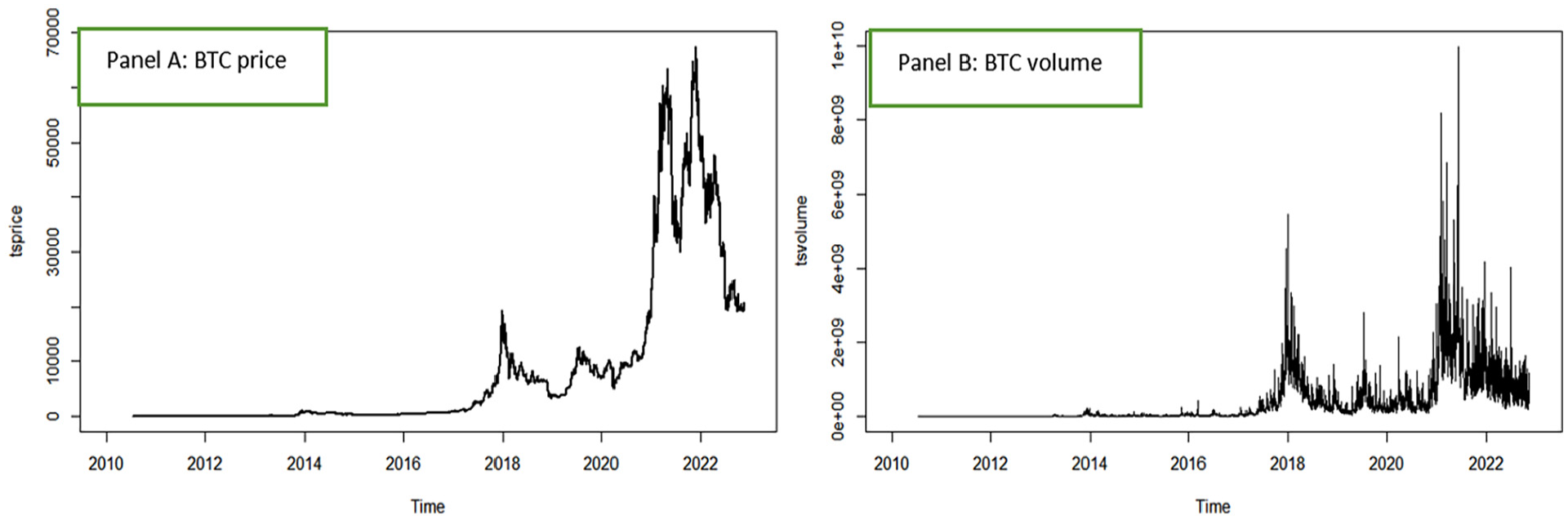
Daily Bitcoin price and trading volume (17/07/2010-31/10/2022).

Empirical Review

Major areas often considered in researching on Bitcoin include forecasting price (Adekunle et al., 2022; Basher & Sadorsky, 2022; A. Demir et al., 2019; Gbadebo et al., 2022; Hamayel & Owda, 2021; Velankar et al., 2018; Ye et al., 2022), jump and co-movements in price (Shen et al., 2020); intraday reversal and momentum effects (Jia et al., 2022; Shen et al., 2020, 2021) and determinants of Bitcoin price (Gbadebo et al., 2021; Jaquart et al., 2021; Koutmos, 2020).

Recent studies assemble alternative approach to forecast the price of Bitcoin. (Basher & Sadorsky, 2022). Basher and Sadorsky (2022) showed that the random forests (RF) model predicts the price with much accuracy than the logit models. The accuracy for the RF model and the bagging classifiers obtained was above 85% for 10 to 20 days forecast and between 75% and 80% for the 5-day predictions. Gbadebo et al. (2022) employed the Exponential Smoothing Model, autoregressive integrated moving average (ARIMA), Neural Network, Seasonal Trend decomposition using Loess (STL), and Holt-Winters filters (HWF) to predict Bitcoin price for three different data periods. The study found that the Naïve model outperforms others models based on the daily price. The results also identified likely evidence that forecasting the price is insensitive to the data periodicity. Ye et al. (2022) used an machine learning model by combining the long short-term memory (LSTM) and Gated Recurrent Unit (GRU) with stacking ensemble system and use sentiment indexes, technical indicators to forecast Bitcoin prices and find that with mean-absolute-error (MAE) of 88.74%, the near-real time forecast reveal better performance.

Adekunle et al. (2022) trained three different datasets (observed data, fitted linear polynomial and fitted generalize STL) on forecasting models, including the ARIMA, HWF and developed 18 models for forecasting daily Bitcoin price. The results showed that the HWF (involving the additive seasonality) with lower limit fitted on STL outperforms based on the first training-sample, while ARIMA (fix) fitted on actual data offers better prediction based on the second training-set. Hamayel and Owda (2021) employed three machine learning methods (GRU, LSTM, bi-LSTM) to predict Bitcoin and Ethereum prices, and found that the GRU model outperforming other algorithms. Jaquart et al. (2021) employed the artificial neural network (ANN), random forests (RF) and LSTM to analyze impact of blockchain, sentiment, technical, and asset returns in explaining Bitcoin price forecasting. The quantile result shows that the long-short trading strategy creates about 39% returns. A. Demir et al. (2019) forecast Bitcoin price using LSTM, Naïve Bayes (NB), and the nearest neighbor technique, attaining prediction accuracy above 80%. Velankar et al. (2018) use the Bayesian regression and generalized linear model to forecast price change signals and uncover an average prediction accuracy of 51%.

Another strand of literature considered issue of Bitcoin time-series intraday reversal effect and price momentum. Shen et al. (2020) introduce a three-factor pricing model for Bitcoin involving market, size, and reversal factors. The paper demonstrates evidence of a reversal effect for the periods. Some other studies suppose the existence of momentum effect and not reversal effect in the markets. For instance, Jia et al. (2022) test a three-factor pricing model including market, size, and momentum factors. The model has a greater explanatory power and outperforms the quasi-cryptocurrency capital asset pricing model based on Shen et al. (2020). Shen et al. (2021) examines momentum effects using Bitcoin price volatility. The study identifies that the first trading window with the highest trading volume or volatility are associated with the greatest predictability for intraday time-series momentum. The intraday momentum trading yields significant economic gains in terms of asset allocations and market timing, especially, in periods that the Bitcoin market experience downturn.

Some studies examined the issue of jump and co-movement tendencies. Shen et al. (2020) investigate the importance of structural breaks and jumps and in forecasting the volatility of Bitcoin price. Using 18 different heterogeneous autoregressive (HAR) models, the paper identifies the significance of decomposing the realized variance in the sample estimation. The finding shows that the HARQ-F-J model is superior to others, an indication that both the squared jump and temporal variation components are important at different time horizons. In addition, across all forecast horizons, the HAR models with structural breaks outperform the models without breaks.

Alaoui et al. (2019b) studied the price–volume cross-correlation and found that identified nonlinear and multifractality interaction theory between Bitcoin price change and changes in trading volume dependence. The multifractality is well-present and significant. Via the GARCH-copula models, M. Naeem et al. (2020) examined the average and extreme returns-volume relation for Bitcoin, Ethereum and Litecoin. The outcome established that the Student-t and time varying symmetrized Joe Clayton copulas optimal for the three cryptocurrencies. The extreme returns are related with extreme trading volumes, and tail dependence is stronger (lesser) for high (low) returns and volumes. Lahiani et al. (2021) use a nonparametric cumulative dependence measure to investigate tail dependence between cryptocurrency and stock returns. The result indicate that the BSE 30 index show the highest predictability of cryptocurrencies but little predictability on stock returns. Amongst cryptocurrencies, Ethereum leads in predictability, followed by Bitcoin.

Some other related studies considered volume as determinants of correlation and spillover cross cryptocurrencies (Bouri et al., 2021; Ji et al., 2019; Shahzad et al., 2021). Bouri et al. (2021) examined market integration among leading cryptocurrencies using the dynamic equicorrelation model. The study found that the evidence of return equicorrelation is very time-varying, and despite sharp price correction during 2018, there is heightened evidence points of integration in the market. Trading volume and uncertainties are found to be main determinants of integration. Shahzad et al. (2021) used the Markov regime-switching model to examine return spillover among 18 cryptocurrencies, while considering three pricing factors and COVID-19 outbreak effects. They found multidimensional patterns of spillover in low and high volatility regimes. The network analysis revealed consistency with contagion theory during stress periods. The evidence exhibits higher spillovers when the volatility was high during COVID-19 outbreak. Ji et al. (2019) explored the connectedness of return and volatility spillover across six large cryptocurrencies. The evidence shows that Bitcoin and Litecoin exhibit strong connection of network of returns. The connectedness via negative returns is stronger than one via positive returns. Ethereum and Dash show weak connectedness via positive returns. Also, the US market’s instability exhibits a positive sign for net directional-volatility spillovers, while gold price shows a negative sign.

Methodology

Data

The Bitcoin (BTC) price used is the United State dollar (USD) price of Bitcoin, denoted as USD/BTC, and the trading volume is in USD. The source of the data is Data.bitcoinity.org database, which is available on the Data.bitcoinity.org’s website. ¹ Following some extant studies on Bitcoin price formation and determinant (Gbadebo et al., 2021; Ji et al., 2021; Jia et al., 2022; Shen et al., 2021; Wang et al., 2022), we applied monthly data which covers the periods spanning 2010:M7-2022:M10. The use of monthly data is justified for the dynamic asymmetric causality testing estimation framework (Hatemi-J, 2012, 2022; Hatemi-J & El-Khatib, 2016). The USD/BTC is the simple unweighted average of the monthly closing price (Gbadebo et al., 2021; Pyo & Lee, 2020). Based on previous studies (e.g., Gbadebo, 2023; Gbadebo et al., 2021; Jia et al., 2022; Pyo & Lee, 2020; Shen et al., 2021; Wang et al., 2022), the price and volume are log transformed. The logarithmic normalization is completed to preserve the cointegration as well as eliminate possible heteroscedasticity is in the series (Pyo & Lee, 2020).

Pre-Tests

First, a preliminary and pre-test evaluation of the data is completed to display the time series plots and corresponding series’ statistics for the log normalization. A pre-test to verify the stochastic property of data generating process (DGP) of each time series is required.

The Augmented-Dickey-Fuller (ADF) and Phillip-Perron (PP) tests verify stationarity. The test identifies each series as I(0) or $I\left(d\right)$ for level [differenced] stationary (where, d is order of integration). Assume $y_t$ ( $x_t$ ) denotes dependent (independent) variable, the ADF uses (1) to verify stationarity for series $x_t$ .

$$x_t=a_0+\phi x_{t-1}+\sum _{i=1}^{p-1}{\delta }_i\Delta x_{t-i}+{\Omega }_t;i=1,2,...,p-1.$$

(1)

Where ${\delta }_i=-\sum _{j=i+1}^{p-1}{\phi }_j$ and $a_0,{\Omega }_t$ and $p$ , respectively, are drift, Gaussian noise, and lag length. The test statistics [ ${\tau }_{\mu }={\hat{\phi }}_T-1/\mathrm{se}\left({\hat{\phi }}_T\right)$ , where $\mathrm{se}\left({\hat{\phi }}_T\right)$ is ${\hat{\phi }}_T^{\prime }$ ’s standard error] is computed using ordinary least squares. The test is performed with the null of non-stationarity ( $H_0:\phi =1$ ) and alternative ( $H_1:\phi >1)$ .

The PP-test allows autocorrelation in $a_t$ , making it white noise, by estimating an “unaugmented” model of (1), allowing for heterogeneity rather than adding up $\left(\sum _{\mathrm{i}=1}^{p-1}\Delta {\mathrm{x}}_{\mathrm{t}-\mathrm{i}}\right)$ , as done in (1). The test defines $\mathrm{\phi }$ in (1) as $\mathrm{\phi }=\sum _{i=1}^p{\phi }_j$ and ${\mathrm{\delta }}_{\mathrm{j}}=-\sum _{j=i+1}^{p-1}{\phi }_j\mathrm{i}=1,2,\dots ,p-1$ , and $k=p-1$ . PP-test modified the ADF[ $\mathrm{Z}\left({\mathrm{\tau }}_{\mathrm{ADF}}\right)]$ to obtain an augmented statistic ( ${\mathrm{\tau }}_{\mathrm{PP}}$ ).

$${\tau }_{PP}={\tau }_{\mu }({\widehat{\sigma }}_{\mu }/{\widehat{\sigma }}_{\mu }-\frac{1}{2}({\widehat{\sigma }}_t^2-{\widehat{\sigma }}_0^2)/{\Sigma }_{\ell }$$

(2)

With: ${\hat{\sigma }}_0^2=T^{-1}\sum _{=1}^T{\hat{a}}_t^2{\hat{\sigma }}_{\ell }^2={\hat{\sigma }}_0^2+2T^{-1}\sum _{j=1}^{\ell }{w}_j\left(\ell \right)\sum _{t=j+1}^T{\hat{a}}_t{\hat{a}}_{t-j}$ )

$${\Sigma }_{\ell }^2=T^{-2}{\widehat{\sigma }}_{\ell }^2\sum _{l=2}^T{(x_{t-1}-1-{\overline{x}}_{-1})}^2$$

(2)

Where, ${\overline{x}}_{-1}=(T-1{)}^1\sum _{t=1}^{T-1}{x}_t$ and $\hat{\mathrm{\sigma }}$ is a consistent estimator of the long-run variance which employs (a kernel function [ ${\mathrm{w}}_{\mathrm{j}}(\ell )]$ as weight of sample autocovariances. The test statistics is compared with a standard limiting distribution critical values. The test checks the null $\mathrm{\phi }=1$ (nonstationary) against the alternative, $\mathrm{\phi }>1.$ The study selects the system’s optimal lag ( $p$ ) required for the parsimonious parameterization of the cointegration test. If the variables are I(1), integrated, the study uses the Johansen (1988) test cointegration under the null of no cointegration.

Considered Method

Vector Autoregression (VAR) System and Impulse Response Function (IRF)

The study determines asymmetric causality evidence for the price-volume relations. Prior to this, the VAR/VECM is employed to depict the inter-dependencies and dynamic relationships of the duo variables. The VAR shows how the endogenous variables are explained by own pasts as well as the current and pasts of the deterministic regressors, is then estimated. The methods is suitable since they incorporate accommodate non-statistical a priori information. $\mathrm{VAR}$ contains set of $K$ endogenous variables $y_t=(y_{1t},\dots ,y_{\mathrm{kt}},\dots ,y_{\mathrm{Kt}})$ . The $\mathrm{VAR}(p)$ -process is defined as:

$$y_t=A_1{y}_{t-1}+\cdots +A_p{y}_{t-p}+u_t$$

(3)

$A_i$ ( $i=1,\dots$ , $p$ ) represent $(K\times K)$ coefficient matrices, $u_t$ is a $K$ -dimensional process with $E(u_t)=0$ and covariance matrix $E(u_t{u}_t^T)={\Sigma }_u$ (white noise). An empirical feature of the VAR(p)-process is its stability based on the eigenvalues of $\mathrm{A}$ in the compact form VAR process:

$${\xi }_t=A{\xi }_{t-1}+v_t,$$

(4)

$$\begin{array}{cc}\multicolumn{1}{c}{{\xi }_{t(\mathrm{KP}\times 1)}}& =\left[\begin{array}{c}\begin{array}{c}{y}_t\hfill \\ \multicolumn{1}{c}{⋮}\end{array}\hfill \\ \multicolumn{1}{c}{y_{t-p+1}}\end{array}\right],A_{(\mathrm{KP}\times 1)}=\left[\begin{array}{ccccc}{A}_1\hfill & A_1\hfill & \cdots \hfill & A_{p-1}\hfill & A_p\hfill \\ \multicolumn{1}{c}{I}& 0\hfill & \cdots \hfill & 0\hfill & 0\hfill \\ \multicolumn{1}{c}{0}& I\hfill & \cdots \hfill & 0\hfill & 0\hfill \\ \multicolumn{1}{c}{⋮}& ⋮\hfill & \ddots \hfill & ⋮\hfill & ⋮\hfill \\ \multicolumn{1}{c}{0}& 0\hfill & \cdots \hfill & I\hfill & 0\hfill \end{array}\right],\hfill \\ \multicolumn{1}{c}{v_{t(\mathrm{KP}\times 1)}}& =\left[\begin{array}{c}\begin{array}{c}{u}_t\hfill \\ \multicolumn{1}{c}{0}\end{array}\hfill \\ \multicolumn{1}{c}{⋮}\\ \multicolumn{1}{c}{0}\end{array}\right]\hfill \end{array}$$

(5)

${\xi }_t$ and $v_t$ are stacked vectors, with dimension $(\mathrm{KP}\times 1)$ and, matrix A has dimension $(\mathrm{Kp}\times \mathrm{Kp})$ . If the moduli of the eigenvalues of $A$ are less than one, the $\mathrm{VAR}(p)$ -process is stable. The evaluate the system with the diagnostic tests (absence of serial correlation, heteroscedasticity or non-normality in the residual process), after estimating the VAR/VECM.

The study presents the impulse response to diagnose the system’s dynamics. The function is based on the Wold moving average representation (Equation 4) for stable $\mathrm{VAR}(p)$ -processes:

$$y_t={\Phi }_0{u}_t+{\Phi }_1{u}_{t-1}+{\Phi }_2{u}_{t-2}+\cdots$$

(6)

with ${\Phi }_0=I_K$ and ${\Phi }_s$ computed recursively using, ${\Phi }_s=\sum _{j=1}^s{\Phi }_{s-j}{A}_j$ for $s=1,2,\dots$ , ), whereby $A_j=0$ for $j>p.$ The forecasts for horizons $h\ge 1$ of an empirical $\mathrm{VAR}$ can be generated recursively based on:

$$y_{T+h|T}=A_1{y}_{T+h-1|T}+\cdots +A_p{y}_{T+h-p|T},$$

(7)

where $y_{T+j|T}=y_{T+j}$ for $j\le 0$ . The forecast error covariance matrix is:

$$\begin{array}{cc}\multicolumn{1}{c}{\mathrm{Cov}}& \left(\left[\begin{array}{c}{y}_{T+1}-y_{T+1|T}\hfill \\ \multicolumn{1}{c}{y_{T+h}-y_{T+h|T}}\end{array}\right]\right)=\left[\begin{array}{cccc}I\hfill & 0\hfill & \cdots \hfill & 0\hfill \\ \multicolumn{1}{c}{{\Phi }_1}& I\hfill & \cdots \hfill & 0\hfill \\ \multicolumn{1}{c}{⋮}& ⋮\hfill & \ddots \hfill & ⋮\hfill \\ \multicolumn{1}{c}{{\Phi }_{h-1}}& {\Phi }_{h-2}\hfill & \cdots \hfill & I\hfill \end{array}\right]\hfill \\ \multicolumn{1}{c}{}& ({\Sigma }_u\otimes I_h)\left[\begin{array}{cccc}I\hfill & 0\hfill & \cdots \hfill & 0\hfill \\ \multicolumn{1}{c}{{\Phi }_1}& I\hfill & \cdots \hfill & 0\hfill \\ \multicolumn{1}{c}{⋮}& ⋮\hfill & \ddots \hfill & ⋮\hfill \\ \multicolumn{1}{c}{{\Phi }_{h-1}}& {\Phi }_{h-2}\hfill & \cdots \hfill & I\hfill \end{array}\right]\hfill \end{array}$$

(7)

⊗ is the Kronecker operator, and matrices ${\Phi }_i$ are the coefficient matrices of the Wold MA decomposition of a stable $\mathrm{VAR}(p)$ -process.

The Causality Tests

Before testing the asymmetric causality, multivariate normality and the heteroscedasticity based on multivariate autoregressive conditional heteroscedasticity-Lagrange multiplier (MARCH-LM) test is confirmed (Lutkepohl, 2006). Afterward, the study presents output for the Toda-Yamamoto (symmetric) causality test. The symmetric causality tests based on the Wiener-Granger process is implemented within the VAR framework, and could infer causality directly from the estimates of the VAR/VECM system. Usually, result from the VECM distinguishes between short and long run (direct) causality. The short (long) run causality is implied if the t-statistics of the regressors (error correction term) in the VECM model are significant. Strong causality is implied if both the t-test of the regressors and the t-test of the error correction model (ECM) term are significant. The exogeneity test give short run causality and the null of no causality is rejected null if the p-value of chi square is less than the .05, supposing the variable does not have any causal relationship at the critical level. The Wald test applies on the coefficients estimated from the cointegration degree (dmax) of the variable that has maximum cointegration (Toda & Yamamoto, 1995). Considering the two variable [ $X_t$ , $Y_t$ ] VAR(p) system as with the case of the Bitcoin price-volume relation. The VAR(p) is:

$$Y_t={\alpha }_0+\sum _1^h{\alpha }_{1i}{Y}_{t-1}+\sum _1^h{\alpha }_{2i}{X}_{t-i}+u_{1,t}$$

(8)

$$X_t={\beta }_0+\sum _1^h{\beta }_{1i}{X}_{t-1}+\sum _1^h{\beta }_{2i}{Y}_{t-i}+u_{2,t}$$

(9)

With, $h=k+q$ , where $\mathrm{k}$ is lag length, and $\mathrm{q}$ is maximum cointegration degree, $u_{1,t}$ and $u_{2,t}$ are estimates of the VAR system’s error residuals. Implying the causality between $X_t$ , and $Y_t$ , the causality test is based on estimate ( ${\alpha }_{2i}$ , ${\beta }_{2i}$ ) of the VAR (p) system (Sims, 1980). The causality test the null ${\alpha }_{2i}=0(\mathrm{i}=1,2,\dots ,\mathrm{p})$ , basically supposing $X_t$ does cause $Y_t$ , and ${\beta }_{2i}$ supposing testing causality that $Y_t$ does cause $X_t$ .

The Hatemi-J causality assumes that positive and negative perturbations exert different impacts. The test transforms and separates the integrated series into positive and negative cumulative terms. If price and volume are I(1) with drift ( $a$ ) and trend ( $t$ ), they are expressed as:

$$\begin{array}{cc}\multicolumn{1}{c}{}& \mathrm{Pbt}{c}_t=a+\mathrm{bt}+\mathrm{Pbt}{c}_{t-1}+{\epsilon }_{1t}\hfill \\ \multicolumn{1}{c}{}& \mathrm{Bvo}{l}_t=a+\mathrm{bt}+\mathrm{Bvo}{l}_{t-1}+{\epsilon }_{2t}\hfill \end{array}$$

(10)

The residual estimates are defined, ${\epsilon }_{1t}=(\mathrm{Pbt}{c}_t-\mathrm{Pbt}{c}_{t-1})-a-\mathrm{bt}$ , and ${\epsilon }_{2t}=(\mathrm{Bvo}{l}_t-\mathrm{Bvo}{l}_{t-1})-a-\mathrm{bt}$ . Equation 10 express as positive and negative partial sums is recursively shown with initial values ( $\mathrm{Pbt}{c}_0,\mathrm{Bvo}{l}_0$ ) as:

$$\begin{array}{cc}\multicolumn{1}{c}{}& {\mathrm{Pbtc}}_{1t}^{+}:=\mathrm{Pbt}{c}_0+\sum _{1=1}^t{\epsilon }_{1i}^{+}\hfill \\ \multicolumn{1}{c}{}& {\mathrm{Pbtc}}_{1t}^{-}:=\mathrm{Pbt}{c}_0+\sum _{1=1}^t{\epsilon }_{1i}^{-}\hfill \\ \multicolumn{1}{c}{}& {\mathrm{Bvol}}_{2t}^{+}:=\mathrm{Bvo}{l}_0+\sum _{1=1}^t{\epsilon }_{2i}^{+}\hfill \\ \multicolumn{1}{c}{}& {\mathrm{Bvol}}_{2t}^{-}:=\mathrm{Bvo}{l}_0+\sum _{1=1}^t{\epsilon }_{2i}^{-}\hfill \end{array}$$

(11)

Recall that positive and negative shocks of random variable ${\epsilon }_t$ (i.e., ${\epsilon }_{1i}^{+},{\epsilon }_{1i}^{-},$ ) are identified as:

$${\epsilon }_{1t}^{+}:=\max ({\epsilon }_t,0):=(\max ({\epsilon }_{1t},0),\cdots ,\max ({\epsilon }_{\mathrm{nt}},0))$$

$${\epsilon }_{1t}^{-}:=\min ({\epsilon }_t,0):=(\min ({\epsilon }_{1t},0),\cdots ,\min ({\epsilon }_{\mathrm{nt}},0))$$

The accumulative positive ( ${\epsilon }_{1i}^{+},{\epsilon }_{2i}^{+}$ ) and negative ( ${\epsilon }_{1i}^{-},{\epsilon }_{2i}^{-}$ ) values would follow:

$$\begin{array}{cc}\multicolumn{1}{c}{{\epsilon }_{1i}^{+}}& =\max ({\epsilon }_{1i},0),{\epsilon }_{2i}^{+}=\max ({\epsilon }_{2i},0),{\epsilon }_{1i}^{-}\hfill \\ \multicolumn{1}{c}{}& =\min ({\epsilon }_{1j},0),{\epsilon }_{2i}^{-}=\min ({\epsilon }_{2i},0).\hfill \end{array}$$

(11)

Asymmetric Granger causality is verified through the Sims’s (1980) VAR(p) system. The Granger causality between any of the four RHS components (i.e., variables in 11) is then separately recognized and verified. For instance, in testing causality between the two positive components (e.g., ${\mathrm{Pbtc}}_{1t}^{+}$ and ${\mathrm{Bvol}}_{2t}^{+}$ ), the VAR(p) consisting of the dependent variables would be defined:

$$\begin{array}{cc}\multicolumn{1}{c}{{\mathrm{Pbtc}}_t^{+}=}& B_0^{+}+B_1^{+}{\mathrm{Pbtc}}_{t-1}^{+}+\cdots +B_p^{+}{\mathrm{Pbtc}}_{t-p}^{+}\hfill \\ \multicolumn{1}{c}{}& +B_{p+1}^{+}{\mathrm{Pbtc}}_{t-p-1}^{+}+v_t^{+}\hfill \end{array}$$

(12)

Where $B_0^{+}$ , $B_r^{+}$ , and $v_t^{+}$ are the 2 × 1 vector of intercepts, 2 × 2 matrix of parameters to be estimated for lag length $r(r=1,\dots ,p)$ and is a 2 × 1 vector of the error terms. The persimmons parameterization of the model requires an optimal lag order (p) suggested by Hatemi-J (2003) using the (Hatemi-J criteria, HJC).

$$\begin{array}{cc}\multicolumn{1}{c}{\mathrm{HJC}=}& \ln \left(\left|{\mathrm{Pi}}_p^{+}\right|\right)+p\left(\frac{n^2\mathrm{lnT}+2n^2\ln \left(\mathrm{lnT}\right)}{2T}\right),\hfill \\ \multicolumn{1}{c}{}& p=1,\dots ,p_{\max }.\hfill \end{array}$$

(13)

$|{\mathrm{Pi}}_p^{+}|$ is the determinant of the variance–covariance matrix of the error terms ( ${\mathrm{Pi}}_p^{+}$ ) in the VAR. The Null that the $\mathrm{jth}$ element of ${\mathrm{Pbtc}}_t^{+}$ does not cause the $\mathrm{kth}$ element of ${\mathrm{Bvol}}_t^{+}$ is tested using the Wald test. The asymmetric causality test critical values materialize from the bootstrapping algorithm with leverage conditions.

Alternative Causality Tests

The literature on causality testing is extensive and many alternatives have been introduced to detect existence of linear and non-linear causality. The Granger (1969) causality test examines only linear causality for bivariate relation between two variables, $X_t$ and $Y_t$ , under the assumption that both time series are stationary. The method tests Causality by including $X_t^{\prime }s$ current values and $Y_t\prime s$ past values. Like the Toda and Yamamoto, the Granger’s (1969) approach requires to first estimate Equations 8 and 9 for a VAR(2) system of Bitcoin price-volume relation. The test is then examined separate for the different equations in the system. For instance, to test Granger causality from $X_t$ to $Y_t$ in Equation 8, the null of no Granger causality is defined as ${\alpha }_{2i}=0$ , and the Wald Chi-Square test statistics is computed and evaluated. The rejection of the null supposes that $X_t$ Granger causes $Y_t$ . The same procedure is completed verify Granger causality from $Y_t$ to $X_t$ for Equation 9. If a variable is Granger-causal in the bivariate model, it may not necessarily be Granger-causal in a larger model of more variables.

The traditional causality test (Granger’s direct causality and Toda and Yamamoto) does account for nonlinearity observed in some time series. Because, some financial and economic variables exhibit nonlinear behavior over-time, ignoring the dynamics could result in misidentification and may reduce the estimation power of the test when examining the relationship between the variables. Depending on the assumption made about the ergodic series, there are different variants of the nonlinear causality test approach. Baek and Brock (1992) developed a nonparametric method to detect existence of nonlinear Granger causality between variables under that the assumption that the variables are exclusively independent and identically. Hiemstra and Jones (1994) modify Baek and Brock (1992)’s nonlinear test by assuming the time series exhibit short-term temporal dependence. Diks and Panchenko (2006) identify that by ignoring the systemic variations in conditional distributions, Hiemstra and Jones accommodate increasing type error though over rejection of the null of non-causality in large sample size. To circumvent the over rejection issue, they suggest that nonlinear causality and nonparametric technique apply for the residuals of the estimated VAR system would offer a more robust information.

Results

Price-Volume Dynamics

Panel A of Figure 2 displays the Bitcoin price for the actual, difference (returns), log transform and log difference (log-returns) for the sample periods (2010:M7–2022:M10) and the Panel B depicts their corresponding plots for the volume series. At least visibly, the actual plots for price and volume appear more likely negatively skewed. Both indicate substantial spiky protrusions, but would be mildly smoothen with the log-scaled normalization. The log transformation is clearly drift and trended upward. The log difference series appear mean reversing. This indicates high volatility and validate sign for nonstationary of Bitcoin price and volume overtime. M. A. Naeem et al. (2021) found that upward trends exhibit stronger multifractality than downward trends.

Figure 2.

Plots of monthly Bitcoin price (Panel A) and volume (Panel B) (2010:M7–2022:M10).

The unit root test is applied to the price and volume series. The results, from ADF and PP implemented, reveal that both variables are non-stationary, in I(0), but become stationary in I(1), supposing they are differenced stationary and integrated. Not surprising, in the cryptocurrency markets, Bitcoin has often experience massive run-up, resistance, reversals, supports and consolidations. Table 1 reports basic statistics for the log of Bitcoin price ( $\mathrm{Pbt}{c}_t)$ and volume ( $\mathrm{Bvo}{l}_t$ ). The correlation between $\mathrm{Pbt}{c}_t$ and $\mathrm{Bvo}{l}_t$ is strong (.963) and significant, suggesting sturdy price-volume co-movement tendency (Alaoui et al., 2019b; M. Naeem et al., 2020). The causal relationships may suppose that the volume contains information about the price, and vice versa, hence specific volume shocks are accountable for certain cyclical price episodes.

Table 1.

Pre-test Information for Bitcoin Price-Volume Data.

VAR	${\mu }_x$	$x_{t.\sigma }$	${\tilde{\mu }}_3$	${\tilde{\mu }}_4$	${\widetilde{\mathrm{JB}}}_{\mathrm{stat}}$	${\sigma }_{x_1{x}_2}$
Panel A: Basic statistics
$\mathrm{Pbt}{c}_t$	2.787	1.496	−0.796	2.912	15.687	-
$\mathrm{Bvo}{l}_t$	8.893	1.705	−1.185	3.647	37.192	0.963*
Panel B: Stationarity test for Bitcoin data
Variable	Deterministic terms	Lag	Test value	Critical values
			[ ${\mathrm{\tau }}_{\mathrm{adf}}$ ]	1%	5%	10%
ADF-test
$\mathrm{Pbt}{c}_t$	Constant, trend	2	−3.472	−4.022	−3.441	−3.145
$\Delta \mathrm{Pbt}{c}_t$	trend	1	−7.774	−3.476	−2.881	−2.577
$\mathrm{Bvo}{l}_t$	Constant, trend	2	−3.147	−4.022	−3.441	−3.145
$\Delta \mathrm{Bvo}{l}_t$	Trend	1	−12.30	−3.476	−2.881	−2.577
PP test			$[{\mathrm{\tau }}_{\mathrm{pp}}]$
$\mathrm{Pbt}{c}_t$	Constant, trend	4	−2.808	−4.022	−3.441	−3.145
$\Delta \mathrm{Pbt}{c}_t$	Trend	1	−7.540	−3.476	−2.881	−2.577
$\mathrm{Bvo}{l}_t$	Constant, trend	3	−2.964	−4.022	−3.441	−3.145
$\Delta \mathrm{Bvo}{l}_t$	Trend	0	−12.30	−3.476	−2.881	−2.577

Source. Author (2022).

Note. Table T1presents the Pre-test estimation information. Data used is taken Data.Bitcoinity.org database, and spans from the seventh month 2010 until the tenth month of 2022. Panel A reports the basic statistics (N, ${\mu }_x,{\sigma }_x,{\tilde{\mu }}_3,{\tilde{\mu }}_4$ ) for the variable $x_1$ (price) and $x_2$ (volume). The Number of observations is 148, $\mu \equiv$ mean, $\sigma \equiv$ Standard deviation, ${\tilde{\mu }}_3\equiv$ Skewness, ${\tilde{\mu }}_4\equiv$ Kurtosis.

*

Indicates test is highly statistical significance at 1% level (using the probability, p $\left|t\right|=0$ ).

JB is the estimate for the Jarque-Bera statistics. If ${\beta }_1$ = 0, the distribution is symmetric and if ${\beta }_2$ < 3, the distribution is platykurtic, if ${\tilde{\mu }}_3$ = 3, mesokurtic or normal and if ${\tilde{\mu }}_4$ > 3, leptokurtic.

For optimal lag (Table 2), the likelihood ration (LR) criterion chooses lag 1, both the final prediction error (FPE) and Hannan Quinn (HQ) criteria suppose lag 2, while Akaike information criterion (AIC) and the Schwarz criterion (SC) unanimously support lag 3. To avoid over-parameterization but ensure system’s parametric parsimony, the study completes robustness check (Table A1) to decide the efficient system for construction of the impulse response. Initially, Lag 1 to 3 are implemented for an unrestricted VAR, and based on the diagnostic tests (Table A4), ² the models with 1 and 2 lags-specification (Tables A2 and A3) appear too restrictive. The stability tests for the time-invariant model with 3 lag-specification indicates no deviations from expected parameter constancy, hence the model is maintained for the cointegration test. The robustness tests suppose that lag 3 is optimal, and the model is likely more parsimonious. The Trace and Max-Eigen tests’ results is provided in Table 2. Irrespective of model type, excluding only when no trend and intercept are involved, 2 co-integrating combinations are significant at 5%. For instance, if both drift and linear trend are considered with 3-lag (Table 3: Panel A), the Trace test statistics ( ${\eta }_r=26.94$ ) and maximum-eigenvalue statistics ( ${\zeta }_{\lambda }=7.160$ ) are slightly lower than the respective critical value, 15.49 and 3.84 at r = 2.

Table 2.

Optimal Lag Selection Tests for Cointegration Parameterization.

Selection criteria	Lag length
	0	1	2	3	4
LR(n)	−	65.73*	38.28	22.55	6.204
FPE(n)	0.402	0.001	0.001*	0.001	0.001
AIC(n)	4.764	−0.859	−1.079	−1.188*	−1.179
SC(n)	4.806	−0.736	−0.873	−0.899*	−0.808
HQ(n)	4.781	−0.809	−1.071*	−0.996	−1.028

Source. Author (2022).

Note. LR = likelihood ration; FPE = final prediction error; AIC = Akaike information criterion; SC = Schwarz criterion; HQ = Hannan Quinn criterion.

LR, maintain lag 1, FPE and HQ supposes lag 2, while AIC and SC criteria unanimously choose lag 3 as optimal. The diagnostic tests are performed to decide the most parsimonious lag for the dynamics of the system’s estimation.

*

Selected optimal lag $(p)$ based on the corresponding criteria. $n$ is number of lag implemented during the specific criterion iteration.

Table 3.

Cointegration Test for the Price-Volume Relations.

Hypothesized no. of CE(s)	Test statistics		Critical values
	p = 3	p = 2	90%	95%	99%
Panel A: Johenson test including intercept and linear trend.Trace: [ ${\eta }_r=T\sum _{i=r+1}^n\ln (1{\lambda }_i)$ ]
r = 0*	26.94	31.77	13.42	15.49	19.93
r = 1*	7.160	12.11	2.706	3.841	6.635
Max-Eigen: [ ${\zeta }_{\lambda }=T\ln |(1{\lambda }_{r+1})|$ ]
r = 0*	19.78	19.66	12.29	14.265	18.52
r = 1*	7.160	12.11	2.706	3.841	6.635
Panel B: Different cointegration test type (summary) by model type
	No intercept	Intercept	Intercept	Intercept	Intercept
Test	No trend	No trend	No trend	Trend a	Trend b
Trace	1	2	2	2	2
Max-Eigen	1	2	2	2	2

Source. Author (2022).

Note. Both Trace and Max-eigenvalue test statistics indicate 2 cointegrating eqn(s) at the .05 level for most tests.

a

Implements linear trend for data.

b

Implements Quadratic trend for data.

*

Denotes rejection of the hypothesis at the 0.05 level. Selected (.05 level*) number of cointegrating relations.

The standardized cointegration equation reflects the Bitcoin price and volume relations obtains 2 cointegrating ranks. Under this circumstance, the VECM would be the suitable and considered to depict the system interdependence to make statistical inference for the relationship. The model, estimated at the optimal lag of the cointegrating regression relates the endogenous variables in the two different models, while estimating the long-run estimates between them and the vector error correction. The dynamics is estimated with a deterministic trend included in the cointegration relation. According to the Wald test completed, the estimation is parsimonious as none of the variable is redundant. Table 4 reports the cointegration matrix’ coefficients $(\beta )$ of the error correction component. This outcome indicate strong positive and significant relationship between Bitcoin price and trading.

Table 4.

Cointegration Matrix (β)’s Coefficients.

	$\beta$
Variable	$\mathrm{Coeff}.$	${\beta }_{\sigma }$	$t$ -stat
$\mathrm{Pbt}{c}_{t-1}$	1.000	-	-
$\mathrm{Bvo}{l}_{t-1}$	−0.925*	−0.049	18.87

*

Indicates statistical significance at 1%.

Table 5 reports the VECM autoregressive system coefficients of the price-volume dynamics. Both price and volume has positive effects on their own deviations and positive influence on shocks of the companion variable. Specifically, the system would suppose that the own price elasticity of bitcoin demand (trading volume) to trading volume is 12.7% in the first period, while the price sensitivity to volume shocks is 8%, in the first period. The outcome may be attributed to two facts: (a) the fact that there is substitution among them during tumultuous episodes, but complementarity in calmer times. (b) investors, traders, and users do wishes to accumulate more volume when the price increase, with hope to hold and sell in nearest future or possible as hedging strategies, sometimes for alternative financial assets that may be plummeting at same time.

Table 5.

VECM Regressions’ Coefficient.

Error correction	$\Delta \mathrm{Pbt}{c}_t\mathrm{Equation}$			$\Delta \mathrm{Bvo}{l}_t\mathrm{Equation}$
	$\mathrm{Coeff}.$	$\sigma$	$p$ -value	$\mathrm{Coeff}.$	$\sigma$	$p$ -value
$\mathrm{Const}.$	0.018***	0.011	.089	0.052***	0.031	.090
$\Delta \mathrm{Pbt}{c}_{t-1}$	0.360*	0.103	.001	0.127**	0.058	.021
$\Delta \mathrm{Pbt}{c}_{t-2}$	−0.258**	0.109	.019	−1.501*	0.317	.000
$\Delta \mathrm{Pbt}{c}_{t-3}$	0.258*	0.098	.009	0.492***	0.286	.086
$\Delta \mathrm{Bvo}{l}_{t-1}$	0.081**	0.037	.030	0.082	0.108	.450
$\Delta \mathrm{Bvo}{l}_{t-2}$	0.038	0.036	.287	0.291*	0.104	.006
$\Delta \mathrm{Bvo}{l}_{t-3}$	−0.011	0.032	.729	0.055	0.095	.562
$\mathrm{EC}{M}_{t-1}$	−0.028*	0.399	.082	−0.239*	0.083	.004
Statistics
${\overline{R}}^2$	.961			.157
$F$ -stat.	157.6			4.795
Criteria
AIC	−1.411			0.720
SC	−1.246			0.885

*

p < .1. **p < .05. ***p < .01.

The significance of the variables indicate that the long-run estimates will be stable, and the short-run dynamics are sustained to the convergence long-run cointegrating equation. The model shows that the cointegration relationship has a reverse shock effects. Excessive price surge beyond the equilibrium constraints in prior period would be adjusted by the error correction to ensure the system equilibrium is maintained. This supposes that any deviation from the equilibrium dynamics due to perturbations in system’s critical variables would be minimized with the correction (Engle & Granger, 1987). The adjustment on the autoregression system reflect convergence of 2% from price to volume and 23.8% from volume to price the following month. Based on Engle and Granger (1987), the coefficients the ECM terms suppose that any 1% deviation between two variables would be minimized with the correction for next month.

The results of all diagnostic tests for the parsimonious model is provided in Table 6, including the graphics of residuals and the multivariable ARCH for the Bitcoin price ( $\mathrm{Pbt}{c}_t$ ) and volume ( $\mathrm{Bvo}{l}_t$ ) equations (Figure A1 and Figure A2, respective, Appendix). The tests are implemented at 5% level. The diagnostic confirms adequacy of the model. The model residuals’ histograms depict a near zero concentration of observations with progressive frequency decline along the tails for both $\Delta \mathrm{Pbt}{c}_t$ and $\Delta \mathrm{Bvo}{l}_t$ equations of the VECM system. Existence of serial correlation of model’s residuals is verify based on the Portmanteau test. ³ Based on the outcome, the null of no serial correlation cannot be rejected. The Eigen values are contained within the unit circle, hence identifying the stability of the model. This is further supported by the ordinary least squares cumulative sum (OLS-CUSUM) visualization. The OLS-CUSUM plot tests for the VECM model are shown in Figure 3 (Panel A: $\mathrm{Pbt}{c}_t$ and Panel B: $\Delta \mathrm{Bvo}{l}_t$ ). The estimates fall inside the critical bands indicating the stability of the long run coefficients. Stability is suitable for the causality analysis. The finding is similar to existing model, but which are based on multivariate VECM and other method. For instance, Gbadebo (2023) show that volume has large influence on Bitcoin price, amongst other considered variables, including mining and network activities. Gbadebo et al. (2021) show how Bitcoin fundamentals, including volume and Google search drive its price swings, while revealing that the market forces leads greater influence than information.

Table 6.

Diagnostic Tests are Conducted for the Model.

	Portmanteau test [Asymptotic]	ARCH [Multivariate]	Normality [Jarque-Bera]
${\mathcal{X}}^2$	93.642* (<0.001202)	145.11* (<2.2e-12)
$\mathrm{JB}$ -stat.			5,905* (<2.2e-16)

Source. Author (2022).

Note. Value in parenthesis are p-values. Based on the LM statistic, the VEC serial correlation cannot reject the null of absence of system’s residuals serial correlation. The MARCH test is significant, hence residuals is not heteroscedastic. The Jarque-Bera statistic fail reject the multivariate normality for the stochastic errors.

*

Indicates statistical significance at 1%.

Figure 3.

Models stability plots. Panel A: OLS-CUSUM of equation pbtc. Panel B: OLS-CUSUM of equation bvol.

Causality Test Analyses

Because the VECM results identifies that Bitcoin price in current month positively intensifies the trading volume value next month, and the reverse is coherent, supposing increase in Bitcoin volume positively influence its price, and by implication bidirectional causality was recognized. To further substantial a formal evidence, the paper applies both Toda-Yamamoto (symmetric) and Hatemi-J (asymmetric) causality tests procedure to confirm potential feedback effects and bidirectional causal dynamic interaction between price and volume. The tests follow from the implemented VECM framework. Table 7 reports the causality test results.

Table 7.

Price-volume [Toda-Yamamoto] Causality Test.

Panel A: Symmetric causality test a
$H_0:X_t\nRightarrow Y_t$		Lag	$F$ -stat.		$p$ -value
$\mathrm{Pbt}{c}_t\nRightarrow \mathrm{Bvo}{l}_t$		2	3.224		.0427
$\mathrm{Bvo}{l}_t\nRightarrow \mathrm{Pbt}{c}_t$		2	24.58		.0018
Panel B: Price-volume [Hatemi-J] asymmetric causality test b
	Test		Bootstrap critical values
$H_0:X_t\nRightarrow Y_t$	Statistics	Lag	1%	5%	10%
${\mathrm{Pbtc}}_t^{+}\nRightarrow {\mathrm{Bvol}}_t^{+}$	9.056*	3	3.237	1.809	7.133
${\mathrm{Bvol}}_t^{+}\nRightarrow {\mathrm{Pbtc}}_t^{+}$	8.110*	2	2.891	3.409	6.348
${\mathrm{Pbtc}}_t^{-}\nRightarrow {\mathrm{Bvol}}_t^{-}$	4.521*	2	3.006	1.729	2.786
${\mathrm{Bvol}}_t^{-}\nRightarrow {\mathrm{Pbtc}}_t^{-}$	7.266**	2	7.731	4.295	4.458
${\mathrm{Pbtc}}_t^{+}\nRightarrow {\mathrm{Bvol}}_t^{-}$	5.187	2	5.605	2.209	7.418
${\mathrm{Bvol}}_t^{+}\nRightarrow {\mathrm{Pbtc}}_t^{-}$	2.939	3	4.587	3.052	4.102
${\mathrm{Pbtc}}_t^{-}\nRightarrow {\mathrm{Bvol}}_t^{+}$	6.896*	3	3.519	5.681	5.690
${\mathrm{Bvol}}_t^{-}\nRightarrow {\mathrm{Pbtc}}_t^{+}$	1.051	2	8.608	5.385	4.131

Source. Author (2022).

Note. ⇏ indicates the causality null (e.g., $\mathrm{Pbt}{c}_t\nRightarrow \mathrm{Bvo}{l}_t$ ; implies that Bitcoin price does not cause the volume). ^aResults from the Toda-Yamamoto causality test. ^bResults from Asymmetric causality. *p < .1; **p < .05. The test transforms $\mathrm{Pbt}{c}_t$ and $\mathrm{Bvo}{l}_t$ into separate into positive and negative cumulative terms. The critical values are generated from the bootstrapping algorithm with leverage conditions.

Consistent with the VECM, the symmetric test reveals that the causality is bidirectional. The direct causality exists from the volume to Bitcoin price, and the test is highly significant at 1%. Likewise, the causality runs from Bitcoin price to volume, and statistically significant but at 5%. The finding is in line with previous studies (Balcilar et al., 2017; Bouri et al., 2019; Koutmos, 2020) that examine causality evidences in connection with multiple variables. For instance, Bouri et al. (2019) show that volume Granger caused returns of cryptocurrencies (Bitcoin, Ethereum, Ripple, Litcoin, Dash, Nem, and Stellar). But, the volume Granger causes return volatility for only Litecoin, NEM, and Dash, when the volatility is low. Balcilar et al. (2017) establish causality between volatility, returns and trading volume of Bitcoin, and find that volume outside of the bearish and bullish market regimes predict the returns. Based on asset pricing factors, Koutmos (2020) identified causality for between Bitcoin price, and other variables including exchange rates, stock prices and interest rate.

Regarding the asymmetric causality, the evidence supposes causality from positive shocks of price ( ${\mathrm{Pbtc}}_t^{+}$ ) to positive shocks of trading volume ( ${\mathrm{Bvol}}_t^{+}$ ) and vice versa. There is causality running from the negative shocks of price ( ${\mathrm{Pbtc}}_t^{-}$ ) to negative shocks of volume ( ${\mathrm{Bvol}}_t^{-}$ ), and from negative shocks of volume ( ${\mathrm{Bvol}}_t^{-}$ ) to the negative shocks of price ( ${\mathrm{Pbtc}}_t^{-}$ ) but at 5% level of significance. In addition, it is evident that the negative shocks of price ( ${\mathrm{Pbtc}}_t^{-}$ ) do cause positive shocks of trading volume ( ${\mathrm{Bvol}}_t^{+}$ ) at the 1% level but the negative shocks of volume ( ${\mathrm{Bvol}}_t^{-}$ ) do not cause positive shocks of Bitcoin price ( ${\mathrm{Pbtc}}_t^{+}$ ). The null of no causality is not rejected for other two cases ( ${\mathrm{Pbtc}}_t^{+}\nRightarrow {\mathrm{Bvol}}_t^{-}$ ) and ( ${\mathrm{Bvol}}_t^{+}\nRightarrow {\mathrm{Pbtc}}_t^{-}$ ). This means there is a unidirectional causality between positive shocks and negative shocks of the series.

Overall, the result supposes asymmetric effect in the return volume relation. The result is plausible, and intuitively, the dissemination and reaction to positive and negative information, as well as their exploding shocks on assets price differ across traders, exchanges, given that Bitcoin involve an open source without any central control (Balcilar et al., 2017). Hence, everyone reacts to volume to transact, based on how the seek opportunities and returns, hence, may cause trading volume Granger-causes price volatility. This behavior is similar to that of stock returns, where the volatility tends to be asymmetric for positive and negative news (Gupta et al., 2022).

Allowing for asymmetry has important implications for the causal inference to avoid spurious causality outcome between underlying variables (Hatemi-J, 2012, 2022; Hatemi-J & El-Khatib, 2016). This is consistent with M. Naeem et al. (2020) and Bouri et al. (2021). For M. Naeem et al. (2020) tail dependence is lesser for high returns and volumes, and is stronger for high returns and volumes, whereas Bouri et al. (2021) indicate Bitcoin return equicorrelation is very time-varying. For the relation, the evidence differs from Balcilar et al. (2017) because the adopted copula-based causality in distribution method uncover different results. Both Shahzad et al. (2021) and Alaoui et al. (2019b) also suggested different result attributed to the different frameworks. Shahzad et al. (2021) non-asymmetric multidimensional patterns of spillover in low and high volatility regimes, especially during COVID-19 outbreak effects. The findings is based on linear and asymmetric relationship, however, Alaoui et al. (2019b) show nonlinear and multifractality interaction between returns and trading volume dependence.

Figure 4 presents the visualization for the Orthogonal IRF. In other to diagnose the models’ dynamic behavior, the IRF are reported for 25 and 50 months different time horizon. Both Bitcoin price and volume would expected to respond to be the shocks from the Bitcoin price different based on the horizon examined. Hence, all figures to the left indicate the response from price shocks, and the figures to the right indicate the response from volume shocks. The Figure depicts the orthogonal impulse response from price shocks to volume. The evidence infer that a 100% shocks on Bitcoin price creates an initial increase impulse response at price (volume). The initial increase impulse response from price is around 10% (0.01%) in the following month, for both the 25- and 50-months horizon, in line with study by Kristoufek (2013). For the 25 months, this would later decline after the third (six) months for the price (volume). In sum, the shock at 100% indicates a positive response for price even up to the 15 months, but this would not be the case for volume, which begins to decline after the sixth month. In sum, the comparative dynamics of the IRF, the study reveals that the effects of the shock either price or volume follows similar part, irrespective of the time horizon examined.

Figure 4.

Orthogonal impulse response from price ( $\mathrm{Pbt}{c}_t)$ shocks to volume ( $\mathrm{Bvo}{l}_t$ ).

Conclusions

The paper uses the symmetric Granger and dynamic asymmetric causality tests to offer insights into a simple and direct relation between Bitcoin price and volume in the cryptocurrency market. Following existing literature, the study confirms stationarity and examine the inter-dependencies between both variables. The dynamic relationship is achieved using the VECM system for the implementation of the impulse response functions and prediction based on the forecast error variance decomposition. The outcomes provide evidence that Bitcoin price and volume are related. Based on the dynamic system, it is found that a strong positive correlation, and a positive Bitcoin price-volume relation exists. The cointegration identify price-volume equilibrium relation, and through VECM, with which the long-run and short-run price-volume dynamics are interpreted, the study recovers evidence of mean reversing systemic perturbations.

The result offers better ways to manage portfolio diversification strategies amongst market participants. The evidence suggest that market participant are now aware that price and volume ae not symmetrical related such that if there is news shocks on price, either positive or negative, they would understand how to react, particularly on the direction of trading volume to mutigate the effects of such news. The paper suggests some recommendations, including to increase more regulatory efforts to curb excessive price fluctuations. Policymakers may achieve this by implementing policies to limit periodic trading transaction to curtail excessive price volatility, and by implication protect investors’ funds.

The paper suggests that future studies may consider the study’s limitations for improvement. Future research may wish to consider larger samples based on daily data (Jiang et al., 2021), especially related to non-linear framework (Diks & Panchenko, 2006). The research may further extend the investigation on the relationships include multiple variables in the analysis of asymmetric. Moreso, to consider how they affect stock markets in emerging economies (Jiang et al., 2021; Lahiani et al., 2021) and the foreign exchange and currencies markets (López-Cabarcos et al., 2021). This is important because sometimes, Bitcoin may be productive tool for portfolio diversification and risk management, hence its activities is sensitive and influence these markets.