Sage Journals: Discover world-class research

Abstract

The predominant way of eliciting risk attitudes is to ask decision-makers to choose between discrete monetary lotteries with known probabilities attached to the payoffs. Yet, arguably, most choices made day-to-day entail continuous outcomes where objective distributions are unknown. This paper investigates responses to continuous “prospects,” employing parametric methods based upon prospect theory under conditions of risk and uncertainty. We find that behavior under uncertainty seemed to mirror that of risk, but there appear to be some differences in how participants dealt with the uncertainty frame compared to risk. Participants appear not to treat “equally likely” outcomes as being “equally likely,” thus demonstrated cumulative probability warping suggested by prospect theory. Participants’ behavior was difficult to fully reconcile with prospect theory, at least to the extent that it is commonly parameterized, perhaps due to endpoints (in particular zero endpoints) being “salient.” Since continuous interval densities have zero mass at zero, this result is curious and has not been reported in experiments using discrete lotteries. We conjecture that although participants on one level understood the nature of the continuous prospects, the format induced a focus on endpoints over and above what would be warranted by the objective distributions given to them.

Keywords

risk uncertainty cumulative prospect theory continuous prospect

Introduction

First, much has been reported about people’s risk attitudes¹ and, to a significant but lesser extent, their attitudes to uncertainty. There has often been an implicit assumption that behavior under risk naturally transfers to behavior under uncertainty, although several studies (e.g., Chateauneuf & Wakker, 1999; Knight, 1921; Sarin & Wieland, 2016; Tversky & Fox, 1995) have provided justification or empirical evidence that individual decision-makers (DMs hereafter) have distinct attitudes to risk and uncertainty.

Second, discrete monetary lotteries with known probabilities attached to the payoffs have been the predominant way of eliciting risk attitudes within an experimental setting. However, many or perhaps most decisions are not about discrete but rather continuous outcomes. Thus, while using discrete prospects may seem convenient to those seeking to elicit risk attitudes, they may be unfamiliar to decision makers.

These two important points regarding the preceding literature, that is, the number of studies skewed toward the measurement of risk compared to uncertainty and the lack of studies investigating attitudes to risk and uncertainty using continuous prospects, motivates this paper. By measuring risk and uncertainty attitudes using continuous prospect experiments, this paper investigates whether there is the potential to examine behavior using the sort of choices that better correspond to the choices people make in their day-to-day lives without placing a significant cognitive burden on respondents.

We obtained our data by conducting a lab-in-the-field experiment, presenting pairs of “interval” or “continuous” prospects to farmers under conditions of risk and uncertainty. Attitudes toward risk, as opposed to uncertainty, were elicited by specifying that all outcomes over a given interval were “equally likely” (i.e., uniform). On the other hand, uncertainty attitudes were elicited by specifying that one outcome within a given interval would be realized but without the specification of an associated probability density or distribution. There is prima facie a case for believing that DMs will treat the probability of outcomes similarly across risk and uncertainty under these conditions. Under Expected Utility (EU), DMs should employ a uniform distribution under risk, whereas under subjective EU (SEU), DMs might employ a uniform distribution under the so-called “principle of insufficient reason” (Sinn, 1980). Our approach under both risk and uncertainty is to estimate respondents’ probability distribution as a generalized beta form (which nests uniformity as a special case).

This paper employs the same parametric structure under both risk and uncertainty. The cumulative prospect theory (CPT) interpretation under risk is that the estimated beta distribution is the consequence of a transformed cumulative uniform distribution, whereas, under uncertainty, the beta distribution represents the subjective distribution employed by respondents. The use of this approach in the context of uncertainty can further be justified given the connection between Choquet EU and (cumulative) prospect theory. As has been shown (in Sarin & Wakker, 1994), the cumulative version of the PT model is equivalent to Choquet EU, where first-order stochastic dominance is preserved. We derive the estimates of the CPT parameters from a Hierarchical Bayesian Logit.

We proceed as follows. In section 2, we review the literature on elicitation techniques, procedural issues, theories, and methods for estimating attitudes to risk and uncertainty. Section 3 discusses the methodologies and outlines the experiment. In section 4, we present the empirical results, discuss the findings in section 5, and conclude the paper in section 6.

Literature Review

The Case for Examining Risk and Uncertainty Attitudes With Non-Standard Subject Pools

Many studies on experimental measures of risk aversion are conducted using student subjects, often referred to as a standard subject pool. However, more accurate measures of risk attitudes and conclusions about the behavior of non-standard subjects (farmers in our case) are obtained if the experimental subjects are farmers rather than a typical subject pool of university students.

In an agricultural context, several decisions are not about discrete but rather continuous outcomes. For example, a farmer’s daily commute time to the farm, the yield of a crop, the change in asset price, or the interest rate on a loan. Besides, risk attitudes have been reported to influence numerous farm decisions, including climate change adaptation strategies (Jianjun et al., 2015), adoption of improved varieties, technologies, and practices adoption (Begho, 2021; Liu, 2013; Simtowe, 2006), crop diversification (Bezabih & Sarr, 2012), off-farm diversification (Ullah et al., 2016) credit (Saqib et al., 2016), saving (Ullah et al., 2015), or insurance (Sherrick et al., 2004).

The ubiquity of uncertainties in agriculture also motivates the focus on examining farmers’ attitudes in this paper. Although there are numerous studies that measure risk attitude with experimental data, there are substantially fewer studies on farmers’ attitudes under uncertainty (Cerroni, 2020 also drew attention to this gap in the literature). Further, several papers in the literature have provided justification for disentangling risk and uncertainty among farmers using experimental methods (e.g., Barham et al., 2014; Bougherara et al., 2017; Cerroni, 2020). These studies, for example, provide evidence that farmers display noisier choices under uncertainty and a greater aversion to uncertainty. In addition, the findings (e.g., Menapace et al., 2016) that farmers’ risk attitudes were not homogenous when elicited from different experimental methods with varying levels of cognitive requirements call attention to the need for research focusing on how risk and uncertainty among non-standard pools are measured.

A Synthesis of the Risk Elicitation Methods and Findings in Previous Studies

Lottery-style tasks have featured significantly in studies of both normative and descriptive decision theories. A considerable number of authors have applied, modified, or adopted the Ordered Lottery Selection designs (OLS), for example, Binswanger (1980), Multiple Price List (MPL) designs, for example, Holt and Laury (2002), Becker, Degroot and Marshak (BDM) Design, for example, Becker et al. (1964), the Random Lottery Pair Designs, for example, Hey and Orme (1994), bespoke methods, for example, Balcombe et al. (2019) among others in real and hypothetical cases.

Many studies have reported inconsistencies when elicitation techniques are applied to artefactual experiments (see Brick et al., 2012; Charness & Viceisza, 2016). Reynaud and Couture (2012), in their comparison of Eckel and Grossman (EG) vs Holt and Laury (HL), also report that risk preferences are affected by elicitation methods. Prokosheva (2016) and Ihli et al. (2013) corroborate this argument by documenting inconsistency in elicitation methods. Other studies have documented different estimates of risk aversion from different elicitation methods.

It has been argued (e.g., in Jacobson & Petrie, 2007; Taylor, 2016) that these inconsistencies arise from people’s cognitive limitations. Comparison between elicitation techniques using the same participants has shown that comprehension plays a role. For instance, the EG method is reported to outperform the HL task in terms of ease of comprehension and reliability (see Dave et al., 2010). Similarly, Cook et al. (2013) reported a high percentage of misunderstanding in a modified HL task, even when an effort was made to modify the task to the level of participants. Csermely and Rabas (2015) corroborated these findings and reported that varying both the possible outcomes and probabilities imposes a cognitive burden that leads to inconsistencies.

Theories for Representing Choices Under Risk and Uncertainty

To model attitudes toward risks and uncertainty, several methods have been proposed. A large number of studies have adopted or modified the EU theory (Von Neumann & Morgenstern, 1944), the SEU theory (Savage, 1954), or the Weighted EU model (Chew & MacCrimmon, 1979; Fishburn, 1983). These theories suggest that DMs choice is determined by comparing expected values, and the EU function is linear in probabilities whether decisions are taken under risk or uncertainty. Although the EU theory (EUT) or its subjective variant arguably remains the benchmark theory of decision-making under risk, EUT or subjective EUT has well-known empirical limitations. Allais (1953), Ellsberg (1961), and Tversky and Kahneman (1981) have discussed these limitations in detail.

Non-EU theories that have shaped the economics literature include Prospect theory (Kahneman & Tversky, 1979), Rank Dependent Utility theory (Quiggin, 1982), Cumulative Prospect Theory (Tversky & Kahneman, 1992), Salience theory (Bordalo et al., 2012), and Regret and Disappointment theories (Bell, 1985; Fishburn, 1984; Loomes & Sugden, 1982). The Cumulative Prospect theory (CPT; Tversky & Kahneman, 1992) combines the concepts of the rank-dependent utility theory with their earlier prospect theory (Kahneman & Tversky, 1979). Although these theories and models have been widely applied, they have not been exhaustively tested in experimental contexts, especially beyond discrete lotteries.

It is likely that the better elicitation methods reflect familiar problems, the better they will induce responses that correspond to “real” behavior. Therefore, our goal is to explore the use of continuous prospects since we contend that many or most of the real prospects faced by DMs are continuous. There have only been a few studies that employ continuous prospects, including Kothiyal et al. (2011) for Prospect Theory, Kontek (2009) for Relative Utility Theory; and Davies and Satchell (2004), Rieger and Wang (2008), Gürtler and Stolpe (2011), Tian et al. (2012), and Nardon and Pianca (2019) for CPT. Notably, none of these studies has focused on extending pairwise continuous outcomes to uncertain prospects. The closest approach to that adopted by this paper is Kontek (2009) which examines risk attitudes only, using both discrete and continuous distributions within the gain, loss, and mixed domains.

Materials and Methods

A Description of CPT for Continuous Prospects

As outlined in Section 2, we follow the cumulative variant of Prospect theory by Tversky and Kahneman (1992), wherein the responses to alternative prospects are dependent on the DM’s sensitivity to outcome and probabilities, and the relative weights the DM assigns to losses and gains. The case of continuous distributions is formalized by Kothiyal et al. (2011) for both risk and uncertainty. In this case, we take a prospect P which specifies the density at any given real finite value x and for which this is a value function v(x) at each point. For this, we can assign a probability that the value will lie within a specified interval X denoted as (P(X)) as:

U (P) = \int_{R +} ω^{+} (P (x \in X (v)) : v (x) \geq τ) d τ - \int_{R -} ω^{-} (P (x \in X (v)) : v (x) \leq τ) d τ

(1)

Where ω denotes a weighting function that differs in the positive and negative domains. The value function we adopt takes the form of a power function in which responsiveness to gains and losses is distinguished by means of the coefficient² $(λ)$ given as:

v (x) = {\begin{matrix} x^{α} \\ - λ {(- x)}^{β} \end{matrix}_{for x < 0}^{for x \geq 0}

(2)

The curvature of the value function for gains and losses is obtained from the parameters $α$ and $β$ , respectively. Under CPT, as outlined above, respondents transform the decumulative distribution in the “Gain domain” and the cumulative distribution in the “Loss domain.” This approach, when combined with the particular transformation function employed by Tversky and Kahneman (1992), implies that (as opposed to linear weighting) small probabilities to the largest gains should be (potentially) overweighted in the Gain domain and small probabilities to the largest loss be (potentially) overweighted in the Loss domain. While this approach has a behavioral interpretation, observationally, it does not matter whether the distorted distribution employed by respondents is derived from a cumulative or decumulative distribution, providing the transformations employed (on either the cumulative or decumulative distribution) allow for outcomes consistent with the overweighting schemes predicted under CPT (e.g., an inverse S transformation for the largest gain in the Gain domain and largest loss in the Loss domain).

Under expected utility and a uniform distribution for all values within a specified region, the equation in (1) collapses to a simple integral of utility over the specified interval, which can be approximated by treating the continuous lottery as a high dimensional discrete lottery (e.g., by assigning equal weight to 100 outcomes equally distributed across the interval). However, assuming the functions $ω^{+}$ and $ω^{-}$ in equation (1) are not uniform, then (1) can be approximated by computing the expected utility where the weights given to each outcome are determined by two beta distributions (one for the Loss domain and one for the Gain domain). Thus, for a continuous prospect for the interval (a,b), the distribution for payoffs (x) is of the Beta form.

f_{gbeta} (x | γ, δ, a, b) = {\begin{matrix} \frac{Γ (γ + δ)}{Γ (γ) Γ (δ)} \frac{{(\frac{x - a}{b - a})}^{γ - 1} {(\frac{b - x}{b - a})}^{δ - 1}}{b - a} \\ 0 otherwise \end{matrix} x \in (a, b)

(3)

Where $Γ (\cdot)$ is the Gamma function and $γ$ and $δ$ are the shape parameters.

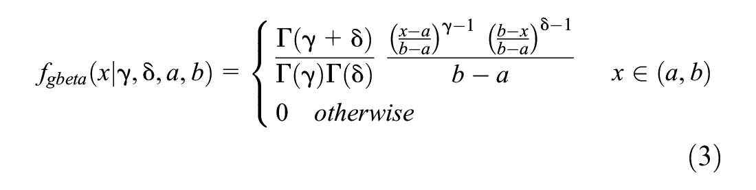
For computation, we treat the continuous lotteries as high dimensional discrete lotteries with probability masses assigned to a set of points spread over a given interval (a, b), with the probability masses given by the beta distribution in equation (3) defined on $γ^{+}$ and $δ^{+}$ in the Gain domain and $γ^{-}$ and $δ^{-}$ in the Loss domain. Therefore, the expected utility under the area defined by the beta distributions converges on that defined under equation (1), nesting the expected utility under uniform distribution as a special case ( $γ$ and $δ$ = 1)

With $V (A)$ and $V (B)$ denoting the systematic utility associated with the prospects A and B, respectively, the probability of choosing prospect A over B is, assuming a random Gumbel error

P (U (A), U (B)) = \frac{1}{1 + e^{- φ (U (A) - U (B))}}

(4)

where the parameter $φ$ (response/choice sensitivity parameter) measures arbitrariness in the DM choice. The closer $φ$ is to zero, the greater the randomness of choices. For details of different value, weighting and choice of functional forms, refer to Stott (2006) and Balcombe and Fraser (2015).

The CPT model estimated in this paper is a hierarchical Bayesian specification that allows for heterogeneous responses across respondents. We formulate a Bayesian prior for a bounded distribution on the vector of parameters $θ$ . The rationale behind setting these bounds is to ensure that the range of the parameters corresponds broadly to results in the existent literature.

Experiment Design and Implementation

The data estimated in this paper was obtained from Nigerian farmers using a lab-in-the-field experiment over continuous outcomes for both uncertainty and risk. In each case, respondents were given finite intervals over which outcomes could occur. The objective density used for the case of risk was a uniform one since this, we believe, is the most understandable form to people unfamiliar with the concept of a probability distribution. By contrast, for the case of uncertainty, no objective distribution for outcomes was specified; therefore, the probabilities of different outcomes were determined by the respondent.

The Prospects Format

The experiment used in this paper was designed to examine participants’ risk and uncertainty attitudes by observing their preference over a series of prospect pairs. We employed seven (7) types of prospect pairs, as presented in Figure 1. In each of the seven (7) types, the top prospect (prospect A hereafter) was more “risky” by having a greater variance than the bottom prospect (prospect B hereafter).

Figure 1.

Types of prospect pairs.

Type 1 is unconstrained in the Gain domain. For example, under conditions of risk, a DM is equally likely to earn any amount between ₦4,280 and ₦7,358 if the DM chooses Prospect A, while for Prospect B, the DM is equally likely to earn any amount between ₦5,361 and ₦6,315. Type 2 has the lower bound of prospect A at zero in the Gain domain. For example, the DM is equally likely to earn any amount between ₦0 and ₦8,662 if the DM chooses Prospect A; while for Prospect B, the DM is equally likely to earn any amount between ₦3,579 and ₦6,108.

Comparing Type 1 to Type 2, it becomes clear that while both are within the Gain domain, the lower limit of prospect A in Type 1 is always greater than zero, unlike Type 2, where the lower limit of prospect A is always “pegged” at zero. In summary, Type 1 is unconstrained in the Gain domain. Type 2 has the lower bound of prospect A at zero in the Gain domain. Type 3 is unconstrained in the Loss domain. Type 4 has the upper bound of prospect A at zero in the Loss domain. Type 5 is unconstrained in the mixed domain. Type 6 has the lower bound of prospect B constrained to zero with Prospect A in the mixed domain, while Type 7 has the upper bound of prospect B constrained to zero with prospect A in the mixed domain. The essence of the different types³ was to cover as many domains and as wide a range as possible.

The prospects were computer-generated random uniform lotteries on the 0 to 100 interval where 0 is the minimum and 100 the maximum values. Several (n = 500) prospects pairs of each of the seven types were generated in the first instance. The utilities and certainty equivalents of the lotteries were then calculated for a ladder of six “anti-symmetric” power utilities which spanned from substantial risk-seeking to strong risk aversion (2|2, 1.25|1.25, 0.99|0.99, 0.5|5, 0.1|0.1, and 0.05|0.05). Prospects pairs were kept if there would be a switch from one of the prospects to another over these range of preferences. Thus, a prospect pair was retained when there was a difference in the certainty equivalents that would ensure there would be a difference in the choices made by participants with different “risk” profiles. Then, the prospect pairs were ranked according to those where switches would be made at different points in the risk preference ladder (for all seven types). Finally, a subset of the prospect pairs was chosen which had a range of switching points at different points in the ladder.

Each participant was required to make a series of choices between Prospects A or B. For the choice tasks, in the beginning, Prospect A had a smaller expected value (EV) compared to Prospect B, and as such, a risk averse participant is expected to choose Prospect B over A. As the EV of Prospect A becomes larger than B in subsequent choice pairs, a risk averse participant is expected to switch to Prospect A from B. However, a unique switching point was not imposed or required. Each participant was presented with a selection of pairs as prospect choice tasks spread across the different content domains under risk and uncertainty. The prospects for risk and uncertainty were largely similar but not identical since we did not wish respondents to simply repeat their choices from one context in another. However, the main difference was the introduction of the “equally likely” concept for the risk experiment, while in the case of uncertainty, this information was not provided.

A pilot⁴ experiment was conducted (using the target group, i.e., smallholder farmers in Nigeria) to determine how well the questions were understood and whether each respondent consistently gave the content of each question the same meaning. The pilot made it possible to identify ambiguous attributes within the experiment. For example, words such as gambles or lottery were frowned upon by respondents of certain cultures and religions; hence we used terms such as prospects in the main experiment.

The “Equally Likely” Concept and Risk Versus Uncertainty

The term equally likely was communicated to participants as a case where all events of a sample space have the same likelihood of occurring. To ensure that respondents understood the concept, we demonstrated “equally likely” with the aid of a wheel spinner. First, we presented a range of possible payoffs, for example, ₦4,280 to ₦7,358, which could be hypothetically earned from a single spin. Then we requested that each respondent pick an outcome randomly within the given interval where they predict the dial would stop after a single spin. We marked “X1,” then randomly picked another spot and marked “X2.” Second, we asked respondents what the chances were that the dial would rest on “X1” compared to “X2” (and compared to any other outcome within the given interval) after a spin. For those who did not provide the right response in the first instance, we repeated the procedure subtly with different outcomes until each participant’s last two consecutive responses were that the spinner was equally likely to rest at any spot.⁵ At this stage, there was no reason for respondents to believe that the chances of occurrence differ between any possible outcome within the interval. After that the decision tasks were presented orally and pictorially to participants, for example,

“Imagine you are faced with a set of monetary prospects as shown. You are equally likely to earn any amount between ₦4280 and ₦7358 if you choose Prospect A. In contrast, you are equally likely to earn any amount between ₦5361 and ₦6315 if you choose Prospect B. Given that you have to make a choice between prospects A or B, which one of the two will you choose?”

As for the case of uncertainty, when a similar set of continuous prospects are presented, the information about probability density is withheld, that is, respondents were told the range of possible payoffs, for example, ₦5,361 to ₦6,315 from which one outcome within the given interval can be realized without any demonstration on the spinner or further information to suggest any probability distribution.⁶

Data Collection Procedure

The participants were 160 smallholder farmers recruited from a random selection of 20 farmers from four Local Government Areas (LGAs) in two States in Nigeria. Respondents were recruited from the list of registered farmers. Each participant had decision-making responsibility on the farm. The experiments were conducted within the LGAs (schools or community halls familiar to participants). Prior, as documented in Begho (2019), ethical approval was granted by the University of Reading, School of Agriculture, Policy and Development - D00108.

The aims and terms of participation were communicated to the participants in English and local languages. Then, the participants were asked if they understood; and whether they consented to these terms. At the beginning of the experiments, a detailed explanation of the necessary concepts (described in sections 3.2.1 and 3.2.2) relating to the choice task was given. We also informed the participants that there was no right or wrong answer.

Participants were informed that one of their prospect choices would be randomly chosen from the Gain domain and played in a consequential way at the end of the experiment.⁷ One of each participant’s choices from the Gain domain was selected and played using a uniform random number generator. The integer had a value between (and inclusive of) the upper and lower bounds of the prospect selected. Similarly, for uncertainty, payment was determined using a random number generator from the Gain domain. On average, the payment to each participant based on the prospect selected was ₦3245 (approximately £7.20). In addition, participants were also given compensation equivalent to an average two-day wage as compensation for time spent and travel costs incurred during the experiment. Notably, participants were not informed beforehand that they would be compensated⁸ for their time to ensure that only those selected and genuinely interested in participating in the experiment took part and avoid any effect the payment would have on their decisions.

Results

The CPT analysis in this section is based on data obtained from 158 participants’ over 35 monetary gains, losses, and mixed tasks resulting in a total of 5,530 risk choices and 5,530 uncertainty choices. The estimates of the individual parameters were derived from a Bayesian mixed logit, but then further inferences about differences across groups were conducted using a classical non-parametric test applied to the respondent specific parameters extracted from the Bayesian mixed logit. The joint posterior parameter distributions estimated in Gauss software were obtained from a Monte Carlo Markov Chain (MCMC) algorithm for 12,000,000 iterations, out of which 2,000,000 iterations were discarded as burn-ins and thus were not used to represent the posterior. In order to reduce correlation across retained posterior draws, 1 in every 1,000 draws was extracted, resulting in a total of 10,000 iterations. Visual observation of the trace plots confirms convergence of the MCMC draws. In line with past studies (Broomell & Bhatia, 2014; Nilsson et al., 2011), this paper imposes restrictions on the CPT parameters presented in Equation 2. The restrictions for both risk and uncertainty are that α∈ [0.05, 2], β∈ [0.05, 2], λ∈ (0.05, 3), γ⁺∈ [0.25, 2], γ⁻∈ [0.25, 2], δ⁺∈ [0.25, 2], δ⁻∈ [0.25, 2], and $φ$ ∈ [0, ∞].

Attitudes to Monetary Risk

The estimated parameters under risk is presented in Table 1. This paper reports both the mean and median values. The results confirm the presence of heterogeneity among respondents (for instance, 25%, 50%, and 75% of the sample have β values of at most 0.12, 0.57, and 1.42, respectively). This is in line with the findings of Abdellaoui et al. (2008) and Resende and Tecles (2011).

Table 1.

Estimated Risk Parameters.

Variables	M	Median	SD	Minimum	25%	50%	75%	Maximum
α	.53	.06	.73	.05	.05	.06	1.30	1.99
β	.76	.57	.68	.05	.12	.57	1.42	1.93
$γ^{+}$	.73	.34	.59	.26	.27	.35	1.33	1.96
$γ^{-}$	.80	.65	.52	.25	.31	.65	1.16	1.90
$δ^{+}$	.71	.45	.52	.25	.29	.45	1.27	1.92
$δ^{-}$	.86	.42	.66	.25	.26	.42	1.58	1.99
λ	1.90	1.90	.97	.50	.84	1.90	2.95	3.00
$φ$	20.87	20.56	16.51	.19	5.52	20.56	34.97	55.87

Note. α, β, and λ parameters of the value function. The curvature of the value function for gains and losses is obtained from the parameters α and β, respectively. The relative sensitivity to gain and loss is measured by λ. The probability parameters are $γ^{+}$ and $δ^{+}$ in the Gain domain and $γ^{-}$ and $δ^{-}$ in the Loss domain. The parameter $φ$ measures arbitrariness in the DM choice.

The results in Table 1 illustrate the non-normality of the distributions of individual preference parameters, also highlighting that reporting the underlying mean and variance parameters alone from the mixed logit would give a misleading impression about overall respondent behavior. We discuss this further when examining the value and weighting functions below.

Utility/Value Function Parameters Under Risk

Figure 2 shows the distribution of α, β, and λ parameters of the value function at the individual level for the case of risk. In line with the definition of risk aversion/seeking with respect to the curvature of the value function, values of 0 < α < 1 and 0 < β < 1 imply risk aversion and risk seeking in the domains of gains and losses, respectively. Figure 2 shows that of the 158 participants, the majority (over 72%) have α < 1 parameter value. This indicates that the curvature of the value function for gains was concave for a majority of individuals. Thus, in line with the definition describing risk aversion in respect of the curvature of the value function, farmers were prevalently risk averse in the Gain domain (although to varying degrees as shown across the different percentiles in Table 1). The distribution of the value function for losses (β) presented in Figure 2 shows that about 54% of participants display a risk seeking attitude toward losses but suggest a mixed picture compared to α.

Figure 2.

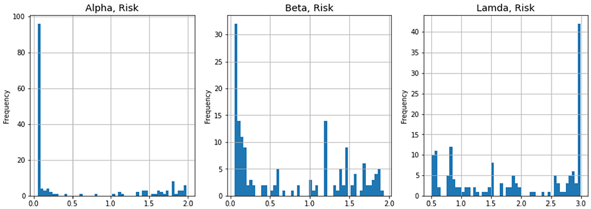
Histogram of the CPT parameters of the value function under risk.

However, the results in Table 1 and distributions in Figure 2 also show that the preferences of many respondents could only be modeled using “extreme curvature” of the value function. Crucially, we observe masses clustered at the lower limit of the restriction for both α and β, which suggests extreme behaviors in the Gains and Loss domains, respectively. We shall return to this point subsequently.

Results regarding the DM’s relative sensitivity to gain and loss (λ) show that participants with λ > 1 made up over 64%. In aggregate, the mean value of λ is 1.90. However, this mean value reflects a kink that is not too “sharp” at the reference point. The mean coefficient is close to the value (λ = 1.87) reported in Booij et al. (2007). However, as discussed in Balcombe et al. (2019), when a symmetry restriction is not imposed on the power parameters, the interpretation of this coefficient is scale-dependent.

Probability Weighting Parameters Under Risk

A common description of probability weightings in terms of a two-payoff discrete prospect CPT weighting scheme in the Gain domain is that people will overweight a small probability of the largest gain and underweight a large probability for the largest gain. However, this type of description does not adequately characterize the nature of the transformations for multi payoff prospects. In a more general setting, the classic “inverse S” type transformation will tend to overweight the upper and lower payoffs and underweight the middle payoffs. When the payoffs are ordered, and the probability mass function is plotted, this will result in a U shape.

The probability distributions employed by respondents under CPT are governed by the interaction of the parameters $γ$ and $δ$ . The clearest way to therefore illustrate the different “probability weightings” used by respondents is to divide them into four groups based on whether the mode of the distribution is bimodal, unimodal, and if so, whether the mode is in the interior of the parameter space or at the left or right extremes. Figure 3 does just this for the risk data, with the Gain domain on the left-hand side and the Loss domain on the right-hand side. Each panel has the range of beta CDFs and PDFs for each of the respondents who fit within that domain (which we label SCDF and SPDF (to denote the subjective nature of these quantities).

Figure 3.

Probability warping by mode of beta distribution under risk.

It is apparent from Figure 3 that very few respondents seem to employ an approximate uniform distribution (which would be consistent with Expected Utility under the “Equally Likely” specification). The top row of panels gives the bimodal distributions for respondents in that category, where both parameters are less than unity. This is the general shape proposed by standard prospect theory. This is the most common distribution employed by respondents (93/158 in the Gain domain and 76/158 in the Loss domain). While this finding supports the hypothesis that participants warp probabilities as in other studies (e.g., Mattos et al., 2007; Tversky & Kahneman, 1992), a substantial number of participants appear to employ distributions that have modes at the left, right, or within the unit interval. Thus, as for the value function parameters, there seems to be considerable heterogeneity across respondents in the way they treat the distribution of outcomes.

Attitudes to Monetary Uncertainty

A description of the estimated parameters under uncertainty is presented in Table 2. In terms of the overall distribution, the estimates broadly reflect the results for the case of risk. However, there are some important differences, as we discuss as follows.

Table 2.

Estimated Uncertainty Parameters.

Variables	M	Median	SD	Minimum	25%	50%	75%	Maximum
α	.57	.09	.72	.05	.05	.09	1.20	1.97
β	.93	.86	.82	.05	.06	.86	1.83	1.99
$γ^{+}$	.81	.37	.66	.25	.30	.37	1.54	1.99
$γ^{-}$	1.15	1.10	.75	.25	.28	1.10	1.97	2.00
$δ^{+}$	.79	.68	.31	.33	.56	.69	1.12	1.57
$δ^{-}$	.94	.68	.68	.25	.26	.68	1.65	1.97
λ	1.87	2.03	.87	.52	1.06	2.04	2.68	2.97
$φ$	13.78	6.18	13.69	.17	1.31	6.18	30.87	41.89

Utility Parameters Under Uncertainty

Figures 4 shows the distribution of α, β, and λ parameters of the value function at the individual level for the case of uncertainty. The majority of the participants, accounting for over 75%, had α < 1 parameter values implying concave curvature of the value function for gains. For the β parameter, about 53% of the estimated value parameter for losses conformed to β < 1. This pattern is similar to the findings in the risk context, where participants were predominantly risk averse for gains and, to a lesser degree, risk seeking for losses.

Figure 4.

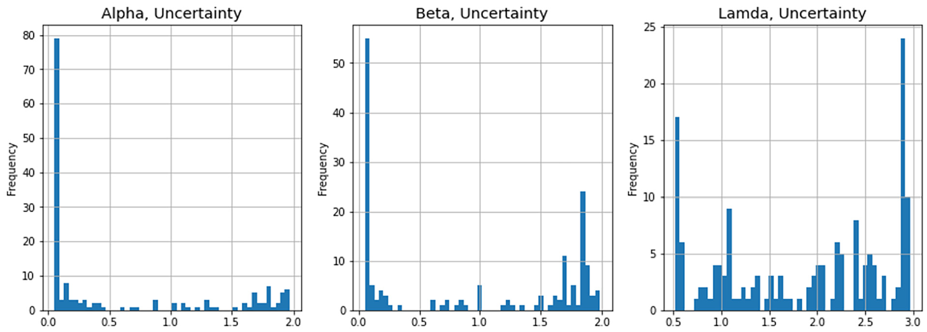
Histogram of the CPT parameters for the value function under uncertianty.

As in the case of risk, the preferences of many respondents could only be modeled using the extreme curvature of the value function. We observe masses clustered at the lower limit of the restriction for both α and β, implying that a large proportion of participants were excessively uncertainty averse in the Gain domain and uncertainty seeking in the Loss domain.

Probability Weighting Parameters Under Uncertainty

For uncertainty, we present in Figure 5 results that are analogous to those for risk in Figure 3. We do not view these as probability transformations but rather as the subjective “capacities” formed by respondents faced with only the knowledge that the monetary gains would lie within a specified interval. For the case of uncertainty, while in the Gain domain, the dominant capacity distribution is again the bimodal beta density, this is not the most common form for the Loss domain, with some respondents appearing to give inordinate weight to the lower boundary, and others to the top boundary. Another third of the respondents have a mode in the interior. Therefore, we conclude that while the mean results look similar, there appear to be some differences in how respondents dealt with the uncertainty frame compared to the risk frame.

Figure 5.

Probability warping by mode of beta distribution under uncertainty.

Comparing Risk and Uncertainty Attitudes

In this section, we examine how the parameters of the models change across the Risk and Uncertainty contexts for the same individuals. There is no strong theoretical basis for believing that the probability weightings or “subjective probabilities” should be similar when dealing with risk as compared to uncertainty, but it is possible that, when faced with interval prospects, individuals treat uncertain interval prospects as being uniform. The results above suggest that this is not the case. Nonetheless, it is useful to examine how “capacities” changed across the risk/uncertainty contexts. In Table 3, we show how people moved across classifications over the two contexts, and in Figure 6, we give similar information in the form of bubble plots. The reason for using the bubble versions is that there were groups of respondents who gave near-identical responses in a given context and therefore had indistinguishable parameters. The bubbles are proportional to the size of responses within a neighborhood of the parameter values.

Table 3.

Probability Parameters Across Risk and Uncertainty.

	Gain domain				Loss domain
Risk\uncertainty	Bimodal	Unimodal left	Unimodal right	Unimodal interior	Bimodal	Unimodal left	Unimodal right	Unimodal interior
Bimodal	50	23	13	7	25	10	24	17
Unimodal left	5	6	0	1	4	20	4	7
Unimodal right	6	0	13	2	2	4	18	2
Unimodal interior	10	1	14	7	5	7	3	6

Figure 6.

Scatter plots of probability parameters across domains.

The results in Table 3 demonstrate that the “modal individual” will be bimodal in both the Loss and Gain domains across both risk and uncertainty. However, the majority of individuals are not “bimodal.” Moreover, the majority of individuals seem to shift typologies when moving from Risk to Uncertainty contexts. This is also illustrated quite starkly by the bubble scatter plots in Figure 6, which clearly do not display a strong correlation.

In Table 4, we present the number of respondents who are both concave or convex across the uncertainty and risk contexts. For example, 95 of the respondents had concave value functions in the Gain domain in both the uncertainty and risk contexts. The two off diagonals show 37 respondents (out of 158) were either concave in the Risk domain and convex in the Uncertainty domains. In addition, 97 respondents (out of 158) are loss averse in both the uncertainty and risk contexts (Table 5).

Table 4.

Consistency across Risk\Uncertainty, Value Function Parameters.

	Gain domain		Loss domain
Risk\uncertainty	Concave	Convex	Concave	Convex
Concave	95	18	64	19
Convex	19	26	25	50

Table 5.

Loss Aversion.

Risk\uncertainty	Loss averse	Non-loss averse
Loss averse	97	25
Non-loss averse	13	23

The degree to which the curvature changes across the Risk/Uncertainty contexts is presented in Figure 7, which gives bubble scatterplots for the parameters across contexts. While there is a weak tendency to have consistent value function parameters across the contexts, overall, there is a substantial shift in the value function across the risk/uncertainty contexts. Given that economists would normally posit a stable value/utility function across risk and uncertainty contexts, this result either points to behavior that is inconsistent with our underlying theory or a model that is simply unable to capture the complexity of individuals responses. We discuss this further.

Figure 7.

Bubble scatter plots of the value function parameters across contexts.

In order to explore people’s behavior, we also classified individuals according to their tendencies to either choose all of the inner prospects (prospect B), all of the outer prospects (prospect A), or switch between the inner and outer prospects at some point; and whether they did this only within the subtasks (e.g., Type 1 and 2 subtasks within the Gain domain tasks). Our first observation was that only 60 out of the 158 people were classified exactly the same way across risk and uncertainty contexts, which again sheds some light on the relative correspondence between the risk and uncertainty CPT results. A common propensity (for around 20% of respondents) was choosing all the inner prospects in the Gain domain and all the outer prospects in the Loss domain while either switching or choosing only the inner prospect in the Mixed domain. To a degree, this is consistent with the CPT treatment of risk aversion in the Gain domain and risk seeking in the Loss domain, along with loss aversion, but more switching should have taken place to be wholly consistent with CPT.

At one end of the spectrum, there were some extreme risk seekers who chose the outer prospect across all tasks (a total of seven respondents for risk and eight for uncertainty). The CPT model accounted for this by estimating a highly convex value function globally. But even so, these individuals required non-uniform probability distributions to explain their behavior at the boundary of the parameter space. At the other end of the spectrum, another group of respondents selected the inner prospect across all tasks (seven in the case of risk and eight in the case of uncertainty). The CPT model dealt with this by assigning a global concavity for the value function and highly non-uniform probability distributions at the boundary of the parameter space. Another small group of individuals (four in the uncertainty case and five in the uncertainty case) always chose the outer prospects in the mixed and Gain domain but always chose the inner prospect in the Loss domain.

The CPT model did not account for this by choosing a convex value function as might have been expected, but rather attributing these individuals with a very high probability “overweighting” at the lower end of the loss interval. Another group were those that tended to always avoid the outer gamble in the Gain domain, but only if it touched on zero (i.e., in Type 2 in Figure 1), and conversely always chose the outer gamble only if it touched on zero (in Type 4 in Figure 1). Such behaviors suggest that a proportion of individuals gave extreme weights to one or both of the endpoints of the intervals, in conjunction with aversion or attraction to zero in the Gain and Loss domains, respectively.

Discussion

When evaluating the model only at the mean, the results seem to broadly conform to the CPT model, being rather similar across risk and uncertainty contexts. However, when evaluating individual estimates, a somewhat different picture emerges. First, the individual’s value function parameters employed here were not stable over the risk/uncertainty contexts (where there is nothing, in theory, to suggest this should happen). Second, many individuals were estimated to have parameters on the edge of the permissible parameter space. The parameter space could be extended. However, this would only serve to illustrate that many respondents behaved in a manner that would normally be considered uncommon relative to the norms found in the literature (e.g., in Nilsson et al., 2011; Broomell & Bhatia, 2014 in terms of the CPT parameters).

Our results provide further evidence consistent with prospect theory in that respondents’ use transformed probability distributions (or their cumulative forms) under risk. However, these results also suggest that the subjective probabilities that respondents employ are not consistent with uniformity even when respondents are told that all points within an interval are equally likely. In short, people do not behave as if all outcomes are equally likely if they are not given any information about the relative likelihood of events, nor if they are told to do so.

Another important aspect uncovered in this study is that in both the risk and uncertainty contexts, farmers were extremely averse to intervals with zero endpoints in the Gain domain while they sought intervals with zero endpoints in the Loss domain. Since continuous interval densities have zero mass at zero, this result has not been found in the preceding literature. Importantly, formally this behavior is not the same as zero aversion (or eagerness for zero) as might be found in response to a discrete lottery where one payoff is zero (see Cettolin & Tausch, 2015; Ert & Erev, 2013). This finding is also difficult to reconcile with standard prospect theory since it requires non-zero probability mass to be placed at discrete points even when respondents are informed this is not the case. Alternatively, it might imply extremely odd behavior in the value function around zero, but such behavior should also be evident in discrete lotteries. Therefore, our contention is that respondents may (practically) place finite mass on salient points, even when those points have zero probability of occurrence.

Our results also support previous findings (e.g., in Andersen et al., 2009; Cerroni, 2020; Sarin & Wieland, 2016) that risk attitudes cannot be directly transferred to attitudes toward uncertainty. This is true not only in the sense that the subjective probabilities employed under uncertainty do not seem to be the same as the probabilities employed under uniform risk (as might be expected) but also that the value functions employed under risk differ from those under uncertainty.

We, therefore, need to reflect on the adequacy of the models employed and/or whether the continuous interval approach has been revealed as a successful mechanism to study respondent behavior toward risk and uncertainty. The different value parameter estimates obtained under risk and uncertainty for the same participant may have arisen from estimating the CPT parameters under a mis-specified model. In particular, while being widely used, the power utility specification may not be sufficiently flexible. Yet, this aside, it remains clear that a number of individuals behaved in a way that was difficult to reconcile with CPT as it is commonly parameterized.

Overall, we conjecture that while the continuous distribution may be more realistic, having a finite domain may have induced respondents to act as if there were discrete masses of probability on the end-points of the intervals. We believe, however, that this is worth further investigation, particularly if there are other “anchors” (such as the mean) in the visual presentation, although it may be that respondents simply focus on boundaries and means, implicitly acting as if there is mass at these points. It could be argued that the results are an “artefact” of design, yet our follow-up⁹ with respondents suggests that this finding should not be dismissed so easily since it did not seem to be the product of misunderstanding by respondents.

Conclusion

At the “mean level,” the estimates that we obtained from the model are consistent with those in the existent literature. However, digging deeper into the nature of individual responses emphasized that mean level results give a very partial picture of people’s behavior and that the tendency of the past literature to work at this aggregate level may have given a misleading impression as to the degree to which aggregate results can be used to infer something about individual behavior.

Our results also show that the distributions used by DMs are not consistent with uniformity under both risk and uncertainty, regardless of whether the objective probability has been specified as uniform. However, we also find that attitudes to risk and uncertainty differ in the sense that few DMs treat interval prospects in the same way if they are specified as having equally likely outcomes (risk) relative to those where the density is undefined (uncertainty).

We also find that cumulative prospect theory only explained individual behavior if people were allowed very convex or concave utility functions and probability distributions that were, in most cases, extremely weighted toward the edge of the prospect intervals. One response to this could be that using discrete prospects continues to be the only way forward. However, our view is that limiting decision theories to discrete choice prospects alone is insufficient for fully understanding attitudes to risk and uncertainty. This calls for a research agenda that improves our understanding of the relationship between formats and responses for both discrete and continuous methods for eliciting attitudes toward risk and uncertainty.

Footnotes

Acknowledgements

The authors would like to thank the anonymous reviewers of the manuscript

Declaration of Conflicting Interests

The author(s) declared no potential conflicts of interest with respect to the research, authorship, and/or publication of this article.

Funding

The author(s) received no financial support for the research, authorship, and/or publication of this article.

Ethical Approval

This research was approved by the University of Reading, School of Agriculture Ethics committee D00108 for S.No: 21015567. Participants were informed that they would participate in the survey and that all data will be de-identified and only reported in the aggregate. All participants acknowledged an informed consent statement in order to participate in the study.

Data Availability Statement

The data that support the findings of this study are available from the corresponding author upon reasonable request.

ORCID iD

Toritseju Begho

Notes

References

Abdellaoui

Bleichrodt

l’Haridon

(2008). A tractable method to measure utility and loss aversion under prospect theory. Journal of Risk and Uncertainty, 36(3), 245–266.

Allais

(1953). Le Comportement de l’homme rationnel devant le risqué: Critique des postulats et axioms de l’école Américaine. Econometrica, 21, 503–546.

Andersen

Fountain

Harrison

G. W.

Rutström

E. E.

(2009). Estimating aversion to uncertainty (Working Paper No. 7-2009). Copenhagen Business School (CBS), Department of Economics. https://research-api.cbs.dk/ws/portalfiles/portal/58999269/wp2009_7.pdf

Azrieli

Chambers

C. P.

Healy

P. J.

(2020). Incentives in experiments with objective lotteries. Experimental Economics, 23(1), 1–29.

Balcombe

Bardsley

Dadzie

Fraser

(2019). Estimating parametric loss aversion with prospect theory: Recognising and dealing with size dependence. Journal of Economic Behavior & Organization, 162, 106–119.

Balcombe

Fraser

(2015). Parametric preference functionals under risk in the gain domain: A Bayesian analysis. Journal of Risk and Uncertainty, 50(2), 161–187.

Barham

B. L.

Chavas

J. P.

Fitz

Rìos-Salas

Schechter

(2014). The roles of risk and ambiguity in technology adoption. Journal of Economic Behavior & Organization, 94, 204–218.

Becker

G. M.

DeGroot

M. H.

Marschak

(1964). Measuring utility by a single-response sequential method. Behavioral Science, 9(3), 226–232.

Begho

(2019). Measuring farmers’ risk and uncertainty attitudes: An interval prospect experiment [PhD thesis, University of Reading, Reading]. https://doi.org/10.48683/1926.00084955

10.

Begho

(2021). Using farmers’ risk tolerance to explain variations in adoption of improved rice varieties in Nepal. Journal of South Asian Development, 16(2), 171–193. https://doi.org/10.1177/09731741211023636

11.

Bell

D. E.

(1985) Disappointment in decision making under uncertainty. Operations Research, 33(1), 1–27.

12.

Bezabih

Sarr

(2012). Risk preferences and environmental uncertainty: Implications for crop diversification decisions in Ethiopia. Environmental and Resource Economics, 53(4), 483–505.

13.

Binswanger

H. P.

(1980). Attitudes toward risk: Experimental measurement in rural India. American Journal of Agricultural Economics, 62(3), 395–407.

14.

Booij

A. S.

van Praag

B. M. S.

van de Kuilen

(2007). A parametric analysis of risk attitudes for the general population under prospect theory (Working Paper). http://dx.doi.org/10.2139/ssrn.1391789

15.

Bordalo

Gennaioli

Shleifer

(2012). Salience theory of choice under risk. The Quarterly Journal of Economics, 127(3), 1243–1285.

16.

Bougherara

Gassmann

Piet

Reynaud

(2017). Structural estimation of farmers’ risk and ambiguity preferences: A field experiment. European Review of Agricultural Economics, 44(5), 782–808.

17.

Brick

Visser

Burns

(2012). Risk aversion: Experimental evidence from South African fishing communities. American Journal of Agricultural Economics, 94(1), 133–152.

18.

Broomell

S. B.

Bhatia

(2014). Parameter recovery for decision modeling using choice data. Decision, 1(4), 252.

19.

Cerroni

(2020). Eliciting farmers’ subjective probabilities, risk, and uncertainty preferences using contextualized field experiments. Agricultural Economics, 51, 707–724.

20.

Cettolin

Tausch

(2015). Risk taking and risk sharing: Does responsibility matter? Journal of Risk and Uncertainty, 50(3), 229–248.

21.

Charness

Viceisza

(2016). Three risk-elicitation methods in the field: Evidence from rural Senegal. Review of Behavioral Economics, 3(2), 145–171.

22.

Chateauneuf

Wakker

(1999). An axiomatization of cumulative prospect theory for decision under risk. Journal of Risk and Uncertainty, 18(2), 137–145.

23.

Chew

S. H.

MacCrimmon

K. R.

(1979). Alpha-nu choice theory: A generalization of expected utility theory. University of British Columbia.

24.

Cook

Chatterjee

Sur

Whittington

(2013). Measuring risk aversion among the urban poor in Kolkata, India. Applied Economics Letters, 20(1), 1–9.

25.

Csermely

Rabas

(2015). How to reveal people’s preferences: Comparing time consistency and predictive power of multiple price list risk elicitation methods. SSRN. http://doi.org/10.2139/ssrn.2573544

26.

Dave

Eckel

C. C.

Johnson

C. A.

Rojas

(2010). Eliciting risk preferences: When is simple better? Journal of Risk and Uncertainty, 41(3), 219–243.

27.

Davies

G. B.

Satchell

S. E.

(2004). Continuous cumulative prospect theory and individual asset allocation (Cambridge Working Papers in Economics 0467). Faculty of Economics, University of Cambridge.

28.

Ellsberg

(1961). Risk, ambiguity, and the savage axioms. Quarterly Journal of Economics, 75, 643–669.

29.

Ert

Erev

(2013). On the descriptive value of loss aversion in decisions under risk: Six clarifications. Judgment and Decision Making, 8(3), 214–235.

30.

Fishburn

P. C.

(1983). Transitive measurable utility. Journal of Economic Theory, 31(2), 293–317.

31.

Fishburn

P. C.

(1984). Foundations of risk measurement. I. Risk as probable loss. Management Science, 30(4), 396–406.

32.

Gürtler

Stolpe

(2011). Piecewise continuous cumulative prospect theory and piecewise continuous hedonic framing. SSRN. http://doi.org/10.2139/ssrn.1965558

33.

Hey

J. D.

Orme

(1994). Investigating generalizations of expected utility theory using experimental data. Econometrica: Journal of the Econometric Society, 62(2), 1291–1326.

34.

Holt

C. A.

Laury

S. K.

(2002). Risk aversion and incentive effects. American Economic Review, 92(5), 1644–1655.

35.

Ihli

H. J.

Chiputwa

Musshoff

(2013). Do changing probabilities or payoffs in lottery-choice experiments matter? Evidence from rural Uganda (GlobalFood Discussion Papers No. 24). Georg-August-Universität Göttingen, Research Training Group (RTG) 1666 - GlobalFood, Göttingen. https://doi.org/10.22004/ag.econ.158146

36.

Jacobson

Petrie

(2007). Inconsistent choices in lottery experiments: Evidence from Rwanda. Journal of Risk and Uncertainty (ExCEN Working Papers No. 114). https://scholarworks.gsu.edu/excen_workingpapers/114

37.

Jianjun

Yiwei

Xiaomin

Nam

P. K.

(2015). Farmers’ risk preferences and their climate change adaptation strategies in the Yongqiao District, China. Land Use Policy, 47, 365–372.

38.

Kahneman

Tversky

(1979). Prospect theory: An analysis of decision under risk. Econometrica, 47(2), 263–292.

39.

Knight

F. H.

(1921). Risk, uncertainty, and profit. Houghton Mifflin.

40.

Kontek

(2009). Lottery valuation using the aspiration/relative utility function. Warsaw School of Economics, Department of Applied Econometrics Working Paper No. 5-09. http://doi.org/10.2139/ssrn.1437420

41.

Kothiyal

Spinu

Wakker

P. P.

(2011). Prospect theory for continuous distributions: A preference foundation. Journal of Risk and Uncertainty, 42(3), 195–210.

42.

Liu

(2013). Time to change what to sow: Risk preferences and technology adoption decisions of cotton farmers in China. The Review of Economics and Statistics, 95(4), 1386–1403.

43.

Loomes

Sugden

(1982). Regret theory: An alternative theory of rational choice under uncertainty. The Economic Journal, 92(368), 805–824.

44.

Mattos

Garcia

Pennings

J. M. E.

(2007). Trading behavior in futures markets: Its determinants and implications [Paper presentation]. Applied Commodity Price Analysis, Forecasting, and Market Risk Management, Chicago, IL, United States.

45.

Menapace

Colson

Raffaelli

(2016). A comparison of hypothetical risk attitude elicitation instruments for explaining farmer crop insurance purchases. European Review of Agricultural Economics, 43(1), 113–135.

46.

Nardon

Pianca

(2019). Insurance premium calculation under continuous cumulative prospect theory. University Ca’Foscari of Venice, Department of Economics Research Paper Series No. 3/WP/2019. https://ssrn.com/abstract=3324183

47.

Nilsson

Rieskamp

Wagenmakers

E. J.

(2011). Hierarchical Bayesian parameter estimation for cumulative prospect theory. Journal of Mathematical Psychology, 55(1), 84–93.

48.

Prokosheva

(2016). Comparing decisions under compound risk and ambiguity: The importance of cognitive skills. Journal of Behavioral and Experimental Economics, 64, 94–105.

49.

Quiggin

(1982). A theory of anticipated utility. Journal of Economic Behavior & Organization, 3(4), 323–343.

50.

Resende

J. G. L.

Tecles

P. L.

(2011). A simple method of elicitation of preferences under risk. Brazilian Review of Econometrics, 31(2), 201–229.

51.

Reynaud

Couture

(2012). Stability of risk preference measures: Results from a field experiment on French farmers. Theory and Decision, 73(2), 203–221.

52.

Rieger

M. O.

Wang

(2008). Prospect theory for continuous distributions. Journal of Risk and Uncertainty, 36(1), 83–102.

53.

Saqib

Ahmad

M. M.

Panezai

Ali

(2016). Factors influencing farmers’ adoption of agricultural credit as a risk management strategy: The case of Pakistan. International Journal of Disaster Risk Reduction, 17, 67–76.

54.

Sarin

Wakker

(1994). Gains and losses in nonadditive expected utility. In Munier

Machina

M. J.

(Eds.), Models and experiments in risk and rationality (pp. 157–172). Springer.

55.

Sarin

Wieland

(2016). Risk aversion for decisions under uncertainty: Are there gender differences? Journal of Behavioral and Experimental Economics, 60, 1–8.

56.

Savage

L. J.

(1954). The foundations of statistics. John Wiley.

57.

Sherrick

B. J.

Barry

P. J.

Ellinger

P. N.

Schnitkey

G. D.

(2004). Factors influencing farmers’ crop insurance decisions. American Journal of Agricultural Economics, 86(1), 103–114.

58.

Simtowe

(2006). Can risk-aversion towards fertilizer explain part of the non-adoption puzzle for hybrid maize? Empirical evidence from Malawi. Journal of Applied Sciences, 6(7), 1490–1498.

59.

Sinn

H. W.

(1980). A rehabilitation of the principle of insufficient reason. The Quarterly Journal of Economics, 94(3), 493–506.

60.

Stott

H. P.

(2006). Cumulative prospect theory’s functional menagerie. Journal of Risk and Uncertainty, 32(2), 101–130.

61.

Taylor

M. P.

(2016). Are high-ability individuals really more tolerant of risk? A test of the relationship between risk aversion and cognitive ability. Journal of Behavioral and Experimental Economics, 63, 136–147.

62.

Tian

Huang

Wang

(2012). Network equilibrium modeling considering the travelers’ risk perception on arrival time [Conference session]. CICTP 2012: Multimodal Transportation Systems—Convenient, Safe, Cost-Effective, Efficient (pp. 457–467). Twelfth COTA International Conference of Transportation Professionals, Beijing , China. https://doi.org/10.1061/9780784412442.04

63.

Tversky

Fox

C. R.

(1995). Weighing risk and uncertainty. Psychological Review, 102(2), 269.

64.

Tversky

Kahneman

(1981). The framing of decisions and the psychology of choice. Science, 211, 453–458.

65.

Tversky

Kahneman

(1992). Advances in prospect theory: Cumulative representation of uncertainty. Journal of Risk and Uncertainty, 5(4), 297–323.

66.

Ullah

Jourdain

Shivakoti

G. P.

Dhakal

(2015). Managing catastrophic risks in agriculture: Simultaneous adoption of diversification and precautionary savings. International Journal of Disaster Risk Reduction, 12, 268–277.

67.

Ullah

Shivakoti

G. P.

Kamran

Zulfiqar

(2016). Farmers versus nature: Managing disaster risks at farm level. Natural Hazards, 82(3), 1931–1945.

68.

Morgenstern

(1944). Theory of games and economic behavior. Princeton University Press. (Second edition, 1947; third edition, 1953. Section 3, chapter I. reprinted in Alfred N. Page. (1968). Utility Theory: A Book of Readings. New York: Wiley, pp. 215–233).

Attitudes to Risk and Uncertainty: New Insights From an Experiment Using Interval Prospects

Abstract

Keywords

Introduction

Literature Review

The Case for Examining Risk and Uncertainty Attitudes With Non-Standard Subject Pools

A Synthesis of the Risk Elicitation Methods and Findings in Previous Studies

Theories for Representing Choices Under Risk and Uncertainty

Materials and Methods

A Description of CPT for Continuous Prospects

Experiment Design and Implementation

The Prospects Format

The “Equally Likely” Concept and Risk Versus Uncertainty

Data Collection Procedure

Results

Attitudes to Monetary Risk

Utility/Value Function Parameters Under Risk

Probability Weighting Parameters Under Risk

Attitudes to Monetary Uncertainty

Utility Parameters Under Uncertainty

Probability Weighting Parameters Under Uncertainty

Comparing Risk and Uncertainty Attitudes

Discussion

Conclusion

Footnotes

Acknowledgements

Declaration of Conflicting Interests

Funding

Ethical Approval

Data Availability Statement

ORCID iD

Notes

References