Sage Journals: Discover world-class research

Abstract

This study tests whether pairs trade conditional on representative bias in the options and stock markets leads to abnormal returns. While previous literature on representativeness focuses on a single index, S&P 500 and Russell 2000 indexes are used to examine the extent to which representative bias arises due to a pattern of similar information shock in the three analyzed periods. The empirical results of the options market lend little support to the representativeness anomalies because Russell 2000 index, relative to S&P 500 index, does not adjust to a sequence of information shocks in the 2020 economic downturn inflicted by the coronavirus pandemic, despite the asymmetrical responsiveness to information shock over the sample period of 2004 to 2020, and during the 2008 global financial crisis. However, the empirical findings of the stock market verify, to some degree, the existence of representative bias during the sample period of 2004 to 2020. To examine whether asymmetrical representativeness in the options market or representativeness in the stock market yields abnormal returns, pairs trade is designed to exploit riskless profits via buying S&P 500 index and selling Russell 2000 index. Based on the Fama and French three-factor model, the empirical evidence is in support of market efficiency because the pairs trading strategy cannot generate positive abnormal returns in both options and stock markets.

Keywords

representative bias pairs trade market efficiency options market

Introduction

The possible existence of such cognitive bias as representativeness is an important issue for financial economists. The market efficiency hypothesis contends that rational investors are not inclined to representative bias and that it is difficult to earn abnormal returns in an efficient market. On the other hand, behavioral finance asserts that people extrapolate too far a series of recent good or bad news about the prospects of companies. Such representative bias may cause price movement substantially upward or downward, and arbitrageurs can earn risk-free profits that arise from a disparity between market prices and fundamental value.

As Poteshman (2001) discovered that options investors exhibit representative bias and overreact to a period of similar information shock, this article takes a step further to investigate whether the degree of misreaction (overreaction or underreaction) resulted from representative bias differs, if any, between Russell 2000 and S&P 500 investors. Russell 2000 and S&P 500 indexes are selected because the financial time series of both indexes, such as option prices, are sufficiently long (i.e., 2004–2020 in this study) to capture relevant key differences between the two types of index fund investors. The empirical model regresses the implied volatility of Russell 2000 index on both the implied volatility of S&P 500 index and prior information shocks observable in the S&P 500 options market. Similar to the methodology proposed by Cao et al. (2005), the information shock is defined as a timeframe of increasing or decreasing daily changes in the implied volatility to be calculated with S&P 500 index option series. A period of steadily ascending (descending) implied volatility is viewed as negative (positive) news for Russell 2000 investors.

The regression results indicate a moderate correlation between the contemporaneous implied volatility of Russell 2000 index and prior information shocks conveyed by the S&P 500 options market. Through the 2004 to 2020 sample period, Russell 2000 investors exhibit underreaction to bad news that is proxied by the ascending implied volatility of S&P 500 index option series. However, Russell 2000 investors are immune from good news that is proxied by the descending implied volatility of S&P 500 index option series, controlling for the level of contemporaneous implied volatility in the S&P 500 options market. The findings that Russell 2000 investors react differently to two sets of information shocks suggest the asymmetrical behavior of Russell 2000 investors.

The empirical analysis also tests how Russell 2000 index, relative to S&P 500 index, responded to extreme and market−wide events, that is, the 2008 global financial crisis and the 2020 coronavirus-induced stock crash. During the 2008 global financial crisis, Russell 2000 investors overreact to good news, but are not responsive to bad news, implying asymmetrical representativeness. More importantly, Russell 2000 investors facing the 2008 global financial crisis reply to information shocks in the opposite manner, compared to Russell 2000 investors in the 2004 to 2020 sample period. As for the 2020 pandemic-caused stock collapse, Russell 2000 investors are indifferent to both positive and negative news, probably because the impact of the coronavirus epidemic on financial markets is still unfolding as time passes. In short, the results of the empirical analysis are inconsistent with the literature on representativeness. The subtle results of asymmetrical representativeness should be viewed with caution since we cannot draw conclusions about the asymmetrical and time-varying traits of Russell 2000 investors. Why Russell 2000 investors display dissimilar response overtime, particularly in 2008 and 2020 volatile markets, deserves further study.

The change in the contemporary implied volatility of Russell 2000 index raises the question whether such a phenomenon matters at the market level. More specifically, could the pairs trade between Russell 2000 and S&P 500 indexes generate risk-free profits? The rationale is that if index fund investors holding Russell 2000 portfolio respond more than their counterparts holding S&P 500 portfolio, arbitrageurs will act swiftly to correct mispriced assets in an efficient market. In search of arbitrage opportunities, a portfolio of pairs trade is considered and calls for buying Russell 2000 index and selling S&P 500 index at the same time when the criteria of representative bias aforementioned are met. The results of the Fama-French three-factor model show that the abnormal return (intercept in the Fama-French three-factor model) of the pairs trade portfolio is statistically insignificant. In view of the efficient markets hypothesis, the above findings suggest that the stock market is so efficient that the securities price quickly incorporates the effect of a succession of public information at a rational level.

As dealing with volatility in the options market, this study also attempts to normalize the time series data by using GARCH (Generalized Autoregressive Conditional Heteroskedastic) models in the stock market. Conditional volatilities are computed in the GARCH (1, 1) specification and the conditional volatilities of Russell 2000 exchange traded fund (ETF) are regressed on conditional volatilities of S&P 500 ETF and prior information shocks observable in the S&P 500 ETF. The regression results suggest that Russell 2000 ETF investors demonstrate representativeness for the full sample period of 2004 to 2020; that is, Russell 2000 ETF investors raise their expectation of riskiness measured by conditional volatility after they witness a series of increasing and decreasing conditional volatilities in the S&P 500 ETF market. A portfolio of pairs trade is also constructed and tested in the Fama-French three-factor model. Similar to the lack of abnormal return in the options market, the abnormal return based on conditional volatilities cannot be found in the stock market, thereby validating the efficient markets hypothesis.

In contrast to most research on representative bias that explores investor misreaction on the basis of stock returns, this is the first paper to probe representative bias by using the implied volatilities in the options market and conditional volatilities in the stock market, and to apply pairs trade by using two broad market indexes, contingent on the time span from 2004 to 2020, and radical market events (i.e., the 2008 global recession and 2020 coronavirus-fueled turmoil). Most studies concentrate on an aggregate index and pay no attention to the abnormal returns resulted from pairs trade. Although the simple trading algorithm (i.e., pairs trading on Russell 2000 and S&P 500 indexes) cannot command abnormal returns, the discovery of a trading approach to exploiting representativeness anomalies, if any, among investors merits further research.

The reminder of this study is organized as follows. The next section reviews the related literature. Section 3 details hypotheses and Section 4 describes methodology. The data and regression results are presented in Section 5 and the robustness check in Section 6. Section 7 outlines implications and limitations and the last section concludes.

Literature Review

A great deal of literature on overreaction in stock markets provides mixed evidence. De Bondt and Thaler (1985, 1987) found that investors tend to overreact to unexpected news events and argue that the mean reversion in which stock prices drift to long-term averages is evidence of overreaction. De Bondt and Thaler (1990) concluded that overreaction stemming from forecasting errors can permeate into the earnings predictions of such stock market professionals as security analysts. On the other hand, Fama (1998) argued that the efficient markets hypothesis is still held because most long-term return anomalies might disappear when we take the methodology problem into account.

Another track of empirical research seeks to investigate misreaction in the options market, instead of stock markets. Stein (1989) contended that long-term S&P 100 index option investors, on average, overreact to new information, compared to short-term S&P 100 index option investors. Some of the empirical research cautions against the evidence of overreaction in the options market because of some methodology problems and the assumption of stochastic volatility of the underlying asset returns. Diz and Finucane (1993) re-examined Stein’s findings by looking at changes in implied volatility, rather than levels of implied volatility for empirical testing, and found little evidence of overreaction.

One school of thought attributes overreaction to the representativeness heuristic. As suggested by the work of Kahneman and Tversky (1973), people may underweigh long-term averages and overemphasize on recent information. After viewing a large number of similar information shocks, investors put too much weight on recent information shocks and ignore long-run fundamental valuation. As a result, the stock price is driven above (below) the equilibrium price and thus overvalued (undervalued) in case of positive (bad) news. The field of behavioral finance underscores the role of the representativeness heuristic in conventional finance models that assume the rationality of investors. Recent articles offer empirical insights into the effect of the representative bias on the decision-making process of investors in the stock markets (Baker et al., 2019; Kanojia et al., 2018; Rasheed et al., 2018; Shah et al., 2018). In a similar vein, Abdin et al. (2017), Bordalo et al. (2019), Isidore and Christie (2019), and Javed et al. (2017) supported the view that the representativeness heuristic is one of the risk factors in predicting stock returns.

A number of studies present evidence of representative bias in the options market. Poteshman (2001) found that long-term option investors overreact to periods of mostly increasing or mostly decreasing daily changes in the instantaneous variance of stock returns. In favor of representativeness, Cao et al. (2005) demonstrated increasing misreaction after four consecutive daily variance shocks of the same sign, either positive or negative. Hibbert et al. (2008) showed that the behavior of traders resulting from representativeness explains the negative correlation between index return and misreaction. However, none of the studies mentioned above links both the representativeness heuristic in the options market and trading opportunities in the stock markets. This paper is the first of its kind to fill this gap in the literature.

One practical application of possible misreaction among investors is to develop profitable trading strategies in asset markets (Hong & Stein, 1999; Goetzmann & Massa, 2002; Rozeff & Zaman, 1998). Pairs trade between two long-term related securities is one of well-known trading algorithms. Recent literature on pairs trading frameworks utilizes a variety of techniques for identifying a set of co-moving securities and falls into three categories: cointegration, stochastic, and artificial intelligence approaches. The cointegration approach centers on cointegration testing to unveil pairs trading opportunities (Clegg & Krauss, 2018; Huang & Martin, 2019; Smith & Xu, 2017). The stochastic approach aims at generating optimal portfolio holdings by different methods of stochastic processes (Farago & Hjalmarsson, 2019; Garivaltis, 2019; Law et al., 2018; Lintilhac & Tourin, 2017; Liu et al., 2017; Tie et al., 2018). The artificial intelligence approach relies on expert and intelligent systems to recognize the attributes of profitable pair combinations (Chaudhuri et al., 2017; Goldkamp & Dehghanimohammadabadi, 2019). A body of empirical evidence supports that a pairs trading strategy results in superior investment performance after accounting for various risk factors (Do & Faff, 2010; Rad et al., 2016; Stübinger & Endres, 2018).

Past studies that examined the representative bias in the stock market suffers from the measurement problem of time-varying risk premium that makes it difficult to gauge the expected return and intrinsic value of an asset. As a result, it is hard to draw a conclusion whether representative bias exists in the stock market, given that investors’ representative bias may be misconstrued based on the uncertainty of the expected return and intrinsic value. Related studies use implied volatility to avoid the problem of time-varying risk premium, but explore the representative bias of only one type of investors in the options market. Also, the literature investigates whether options traders overreact to information, but does not examine the dynamic changes in overreaction and whether overreaction warrants the abnormal return; namely, positive alpha. This paper adds to the literature on behavioral finance through the lens of arbitrage trading profits resulting from misreaction, and intends to evaluate the representative bias between two types of investors in the options market, and whether such representative bias leads to arbitrage opportunities in the stock market.

This research attempts to explore two types of investors (large capitalization vs. small capitalization investors) and is motivated by Berk et al. (1999) that highlights the systematic difference between small stocks and large stocks. They describe market capitalization as a variable that captures the relative importance of existing assets versus growth opportunity of a company. In the United States, two of the most popular stock market indexes are the S&P 500 and the Russell 2000 indices, given that both equity indices are designed to measure the market performance of U.S. stocks. Ivanov et al. (2013) show a positive correlation between S&P 500 and Russell 2000 indices in the spot, futures, and exchange traded funds (ETF) markets. Two major differences between both indices are the size of market capitalization and the style of portfolio construction (Shankar, 2007). First, Russell 2000 index tracks small-capitalization (small-cap) stocks while the S&P 500 index, on the other hand, track large-capitalization (large-cap) stocks. The S&P 500 index is widely recognized as a bellwether for the overall US economy as it features 500 leading U.S. publicly traded companies, with a primary emphasis on market capitalization. The Russell 2000 index is a market index comprised of 2,000 small-cap companies and is frequently used as a benchmark for U.S. small-cap sector. Second, in terms of the style of portfolio construction, S&P 500 index is an actively constructed portfolio since the managers of S&P 500 index exercise discretion in selecting component stocks for the S&P 500 index from a pool of eligible companies. In contrast, Russell 2000 index is a passively constructed portfolio since the managers of Russell 2000 index use nondiscretionary approach to selecting constituent stocks solely based on market capitalization.

To summarize, the research question is whether the representative bias measured by the magnitude of investors’ misreaction, hinges on the arrival of information shock which is proxied by the periods of most increasing or decreasing implied volatilities. A pairs trading strategy is constructed to assess the existence of riskless profits, if any, as detailed in the subsequent section along with two hypotheses.

Hypotheses

Market participants usually react to contemporary information in a timely manner. If a string of the previous information is consistent with (contradictory to) the current information, market participants may reinforce (discount) their assessment about the impact of the current information on asset prices, thereby leading to representative bias. In other words, the content of the increasing (decreasing) pattern of the previous information may be treated as a piece of new information (or information shock) that exacerbates investors’ reaction to the recent information. The first hypothesis is called excessive responses hypothesis and tests whether the up-to-date Russell 2000 implied volatility increases (decreases) with an upward (downward) movement of the S&P 500 implied volatility; that is, Russell 2000 traders overreact (underreact) to the information shock, proxied by the rising (descending) S&P 500 implied volatility. In the context of representativeness anomalies, the excessive responses hypothesis states that Russell 2000 traders, relative to S&P 500 traders, respond more excessively to a string of recent information shocks than they otherwise would under a random arrival of information. Rather than using the price movement of options as a proxy for information shock, the information shock is attained in the upward or downward direction of the implied volatility of S&P 500 index options over a window of five trading days. The implied volatility is a better measure of investors’ reaction than options price because it reflects the unbiased, risk-neutral volatility derived from the options contract.

The second hypothesis is called sensitivity to information hypothesis and aims to tests whether arbitrageurs earn profits by short selling (buying) Russell 2000 index shares when the overaction (underreaction) of Russell 2000 traders, who face information shock embedded in a wave of elevating (abating) S&P 500 implied volatility, makes Russell 2000 index overpriced (underpriced). The sensitivity to information hypothesis asserts that the sensitivity of Russell 2000 traders to a succession of information leads to risk-free profits. This study follows the lead of the pairs trade literature to investigate the existence of abnormal returns that could be resulted from representativeness. A pairs trading method that simultaneously short sells Russell 2000 index and buys S&P 500 index can hedge, to some degree, the adverse effect of the general market direction on the performance of individual indexes. A drop in the stock market will hurt the long position in the S&P 500 index, but benefit the short position in the Russell 2000 index, and vice versa. The long and short positions inherent in the pairs trade provide a hedge against each other (Lakonishok et al., 1994; La Porta et al., 1997). In sum, the mechanism of pairs trade conditional on representative bias may exploit the suboptimal behavior between Russell 2000 and S&P 500 investors, and yield riskless returns. The next section discusses the methodology that outlines the Black–Scholes option pricing model to compute the implied volatility, and the Fama and French three-factor model to calculate the abnormal return.

Methodology

The Black–Scholes option pricing model (Black & Scholes, 1973) is a model to value an option that use the stock price, the risk-free interest rate, the exercise price, the time to expiration, and the standard deviation of the stock return. The respective Black–Scholes option pricing formulas for a European-style call and put option are described as:

C_{0} = S_{0} e^{- δ T} N (d_{1}) - X e^{- r T} N (d_{2})

(1)

p_{0} = X e^{- r T} N (- d_{2}) - S_{0} N (- d_{1})

(2)

where

\begin{array}{l} d_{1} = \frac{\ln (\frac{S_{0}}{X}) + (r - δ + \frac{σ^{2}}{2}) T}{σ \sqrt{T}} \\ d_{2} = d_{1} - σ \sqrt{T} . \end{array}

C₀ is the call option value, P₀ is the call option value, and S₀ is the stock price at time 0. The cumulative normal distribution function, N(d), is the probability that a random draw from a standard normal distribution will be less than d. X is the exercise price, δ is the annual dividend yield of the index, and r is risk-free interest rate. T is the time (in years) remaining until expiration of the stock option and σ is the standard deviation of the stock return.

The first four inputs of Black–Scholes option pricing formula (S₀, X, r, and T) are directly observable from financial markets. Academics and practitioners often appraise the last parameter, the standard deviation (σ) of the stock return, that is consistent with the market value of the corresponding options. The estimated value of the standard deviation of the stock return, referred to as implied volatility, is the volatility level for the stock implied by the option price. Put differently, implied volatilities are the volatilities estimated by stock option prices observed in the market. Traders uses implied volatilities to monitor the market’s opinion about the volatility of a particular stock, and determine whether the stock option is over- or under-valued by comparing actual standard deviation with the implied volatility. If actual standard deviation is less than the implied volatility, the option’s intrinsic value will be below the option price and the option contract will be considered a good buy; if actual volatility exceeds the implied volatility, the option’s fair value will be above the option price and the option contract will be considered a bad deal.

The Black–Scholes option valuation formula is utilized to compute the implied volatility (IV) that measures the market’s expectation of 30-day volatility implied by at-the-money Russell 2000 index and S&P 500 index option prices, respectively. Let IVRussell 2000 and IV_{S&P 500} denote the implied volatility for Russell 2000 index and S&P 500 index, respectively. The following equation is deployed to assess the degree of representative bias:

\begin{array}{l} I V_{Russell 2000} = β \times I V_{S & P 500} + {δ^{+}}_{1, IV} \times PI {S^{+}}_{1} + {δ^{+}}_{2, IV} \\ \times PI {S^{+}}_{2} + {δ^{+}}_{3, IV} \times PI {S^{+}}_{3} + {δ^{+}}_{4, IV} \\ \times PI {S^{+}}_{4} + {δ^{+}}_{5, IV} \times PI {S^{+}}_{5} + {δ^{-}}_{1, IV} \\ \times PI {S^{-}}_{1} + {δ^{-}}_{2, IV} \times PI {S^{-}}_{2} + {δ^{-}}_{3, IV} \\ \times PI {S^{-}}_{3} + {δ^{-}}_{4, IV} \times PI {S^{-}}_{4} + {δ^{-}}_{5, IV} \times PI {S^{-}}_{5} \end{array}

(3)

IVRussell 2000 is regressed on both IV_{S&P 500} and previous information shocks (PIS), assuming that Russell 2000 investors respond to a series of public information embedded in the positive or negative tendency of S&P 500 implied volatility. PIS⁺_t (PIS⁻_t) is a dummy variable for the upward (downward) movement of S&P 500 implied volatility during the time interval t and the superscript + (−) represents the positive (negative) trend of IV_{S&P 500}. Specifically, PIS⁺_{t = 1, 2, 3, 4, or 5} (PIS⁻_{t = 1, 2, 3, 4, or 5}) will take on the value of one if S&P 500 implied volatility successively moves upward (downward) in the previous 1, 2, 3, 4, or 5 trading days, and otherwise take on the value of zero. The respective coefficients δ⁺_{t = 1, 2, 3, 4, or 5, IV} (δ⁻_{t = 1, 2, 3, 4, or 5, IV}) measure the degree of misreaction or representative bias when Russell 2000 investors observe the increasing or decreasing evolution of S&P 500 implied volatility in the past five trading days. The subscript IV of δ⁺_{t, IV} coefficients stands for implied volatility. The time span of five trading days is chosen as the threshold for the PIS dummy variables because there are no records of increasing or decreasing pattern of S&P 500 implied volatility beyond five trading days.

The capital asset pricing model (CAPM) was developed by Sharpe (1964) and is a widely recognized financial model that determines the market equilibrium price and the appropriate measure of risk for a single asset. The CAPM theorizes the risk factor as beta that is a function of the security’s covariance with the market portfolio. However, financial economists (Bhandari, 1988; Roll, 1977) found stock market anomalies for the CAPM, and cast doubt upon the applicability of the CAPM for being an effective model in explaining stock market returns. Fama and French (1992, 1996, 2004) established a milestone model that consists of beta, size effects, and the book to market ratio, in order to test the CAPM on the cross-sectional relationship between risk and return. They interpret both size effects and the book to market ratio as risk factors, in addition to beta. Therefore, this study adopts the Fama and French three-factor model as the approach to estimating the abnormal return on the pairs trade between Russell 2000 and S&P 500 indexes shown below:

R = α + β_{M} R_{M} + β_{S M B} R_{S M B} + β_{H M L} R_{H M L}

(4)

where R is the excess return on the pairs trade on a daily basis when the condition of representative bias is met. Precisely, R is the total return as a result of simultaneously short selling Russell 2000 index and buying S&P 500 index if S&P 500 implied volatility exhibits upward or downward trend within five trading days. Once PIS⁺_t or PIS⁻_t dummy variables take on the value of one, R is computed as the sum of the return on the S&P 500 long position and Russell 2000 short position. The return on the S&P 500 long position is calculated as (P_t_+ 1 − P_t)/P_t or close price at time t + 1 minus close price at time t divided by close price at time t. The return on the Russell 2000 short position is calculated as (P_t − P_t_+ 1)/P_t or close price at time t minus close price at time t + 1 divided by close price at time t. Notice that both short and long positions are reversed on the following trading day for the pairs trade portfolio and that the close price of iShares Russell 2000 ETF (ticker: IWM) and SPDR S&P 500 ETF (ticker: SPY) are chosen to calculate the excess return because the two ETFs constitute the most liquid U.S. ETF market and well represent Russell 2000 and S&P 500 indexes, respectively. α is the abnormal return, and R_M is the market risk premium. R_SMB measures the return on a portfolio consisting of small stocks in excess of the return on a portfolio consisting of large stocks, and R_HML measures the return on a value portfolio in excess of the return on a growth portfolio.

Data and Regrssion Results

There are two datasets of daily options on the ETFs: iShares Russell 2000 ETF and SPDR S&P 500 ETF that are proxies for small- and large-cap portfolio, respectively. The daily close prices of both iShares Russell 2000 ETF and SPDR S&P 500 ETF, and options datasets are obtained from the Chicago Board Option Exchange. Options datasets consists of daily close price, the exercise price, the time to expiration, open interest, and trading volume for call and put contracts. Data on risk-free interest rates is obtained from the St. Louis Federal Reserve web site. Given the option price, the risk-free interest rate, the exercise price, the time to expiration, daily implied volatilities are inferred by equations (1) and (2) for call and put options, respectively.

Table 1 reports the summary statistics of average implied volatilities of call and put options. There are 4,175, 756, and 150 daily observations of implied volatilities for the full period of January 2, 2004 to August 5, 2020, the first subperiod of January 3, 2007 to December 31, 2009, and the second subperiod of January 2, 2020 to August 5, 2020, respectively. The first subperiod of 2007 to 2009 corresponds to the 2008 Great Recession characterized by a period of global recession observed in national economies that occurred between 2007 and 2009. According to the U.S. National Bureau of Economic Research (NBER), the 2008 Great recession began in December 2007 and ended in June 2009. Following the end of credit and housing boom in 2006, the first subperiod extends over 2 years from 2007 to 2009 because there were an exorbitant rise (decline) in asset prices and interest rates before (after) the 2008 Great Recession (Baglioni & Monticini, 2010; Flannery et al., 2013). The first subperiod should be long enough to examine the learning behavior of investors concerning earlier credit excesses, re-pricing of risks, and aftermath of financial market turmoil throughout the 2007 to 2009 financial crisis. As the datasets were collected in August 2020, the second subperiod spans from January 2, 2020 until August 5, 2020 because most economies globally registered sharp rates of contraction as a consequence of coronavirus-led lockdowns since March 2020 followed by a V-shaped economic recovery in terms of Gross Domestic Product (GDP). According to the NBER, recognized as the official arbiter of economic cycles, the 2020 downturn induced by COVID-19 featured a staggering 31.4% GDP plunge in the second quarter of 2022, and was followed by a remarkable 33.4% GDP growth in the third quarter. The length of the second subperiod should be sufficient to study the representative bias of investors during the outbreak of COVID-19 pandemic. Regardless of the three periods considered in the analysis, all statistics of the Russell 2000 index option dataset are higher than those of the S&P 500 index option dataset. Higher statistics of the implied volatility of the Russell 2000 index are consistent with the notion that Russell 2000 index are perceived as being riskier and more volatile than S&P 500 index.

Table 1.

Summary Statistics of Implied Volatility.

Sample period	No. of observed	M	Implied	Volatility	Maximum	Minimum
Sample period	No. of observed	M	Median	SD	Maximum	Minimum
2004−2020
Russell 2000	4,175	24.04	20.86	10.08	87.62	11.83
S&P 500	4,175	18.71	15.78	9.26	82.69	9.14
2007−2009
Russell 2000	756	33.31	29.82	13.77	87.62	14.44
S&P 500	756	27.21	23.95	13.19	80.86	9.89
2020
Russell 2000	150	38.35	38.92	16.21	83.19	13.35
S&P 500	150	31.57	28.61	15.19	82.69	12.10

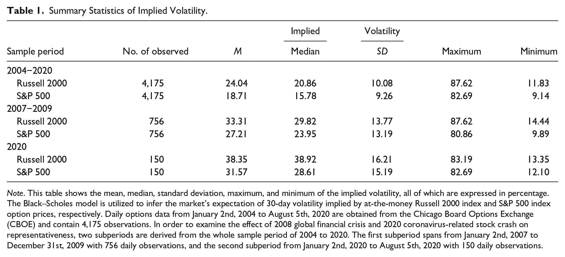
Note. This table shows the mean, median, standard deviation, maximum, and minimum of the implied volatility, all of which are expressed in percentage. The Black–Scholes model is utilized to infer the market’s expectation of 30-day volatility implied by at-the-money Russell 2000 index and S&P 500 index option prices, respectively. Daily options data from January 2nd, 2004 to August 5th, 2020 are obtained from the Chicago Board Options Exchange (CBOE) and contain 4,175 observations. In order to examine the effect of 2008 global financial crisis and 2020 coronavirus-related stock crash on representativeness, two subperiods are derived from the whole sample period of 2004 to 2020. The first subperiod spans from January 2nd, 2007 to December 31st, 2009 with 756 daily observations, and the second subperiod from January 2nd, 2020 to August 5th, 2020 with 150 daily observations.

Because the implied volatilities of both indices are time series data, it is necessary to check whether the implied volatility series is stationary before applying ordinary least squares (OLS) regression specified by equation (3). If taking a non-stationary time series as if it were stationary, traditional time series regression models with this stationary assumption will yield spurious estimations. The Dickey-Fuller test (Dickey & Fuller, 1981) is a way to detect the presence of non-stationary property (or a unit root) in the time series data. The null hypothesis (H₀) of the Dickey-Fuller test stipulates that the implied volatility series has a unit root and the alternative hypothesis (H_A) states that the implied volatility series does not have a unit root. Under the assumptions of no constant term and no linear deterministic time trend, the Dickey-Fuller test provides that the calculated tau statistic (τ) values are −5.78 and −6.62 for Russell 2000 and S&P 500 implied volatility series, respectively, and less than the critical tau statistics (τ_critial) value of −3.43 at the 1% significance level. Thus, the empirical evidence of the Dickey-Fuller test rejects the null hypothesis that both implied volatility series are not stationary. Not reported here, the results of Dickey-Fuller test, assuming a constant term and no linear deterministic time trend, also rejects the null hypothesis and accept the alternative hypothesis (H_A) that Russell 2000 index and S&P 500 implied volatilities exhibit stationary property. Hence, the OLS regression outlined in the following paragraph is an appropriate model specification for stationary time series of Russell 2000 index and S&P 500 implied volatilities.

In equation (3), the effect of representativeness on Russell 2000 investors is explored by regressing IVRussell 2000 on both IV_{S&P 500} and previous information shocks (PIS), including PIS⁺_{t = 1, 2, 3, 4, or 5} and PIS⁻_t =_{1, 2, 3, 4, or 5}. Table 2 shows the regression results of equation (3). All coefficient estimates of IV_{S&P 500} in the three evaluated periods are larger than one and statistically significant, with p values less than 0.1. The regression coefficient β being greater than one suggests either that Russell 2000 investors react more than S&P 500 counterparts or that the instantaneous implied volatility of Russell 2000 index is more volatile than S&P 500 index. Over the full sample period of 2004 to 2020, the coefficient estimations of PIS⁺ are negative and statistically significant. The negativity of these five estimated coefficients that are composed of δ⁺_{1, IV} to δ⁺_{5, IV} may be construed as evidence of representativeness in a way that Russell 2000 investors who face a series of similar information shocks lessen their expectation of implied volatility. The results of insignificant coefficients (δ⁻_{1, IV} to δ⁻_{5, IV}) reveal that Russell 2000 investors are neutral to a series of information shocks (i.e., a decreasing trend of S&P 500 implied volatility). The significant coefficients in the δ⁺_IV group, in contrary to insignificant coefficients in the δ⁻_IV group, point to asymmetrical representativeness, but invalidate the representativeness heuristic as a whole.

Table 2.

Regression Results of Implied Volatility.

Coefficient	Sample period
Coefficient	2004−2020	2007−2009	2020
b	1.06***	1.04***	1.01*
δ ⁺ _{1, IV}	−0.93*	0.87	−5.48
δ ⁺ _{2, IV}	−1.15**	0.33	−6.70
δ ⁺ _{3, IV}	−1.36***	0.05	−11.86**
δ ⁺ _{4, IV}	−1.00*	0.00	N/A
δ ⁺ _{5, IV}	−1.57***	−2.01	N/A
δ⁻_{1, IV}	−0.83	1.02*	−5.58
δ⁻_{2, IV}	−0.70	1.22**	−3.23
δ⁻_{3, IV}	−0.72	1.36**	−3.50
δ⁻_{4, IV}	−0.48	2.04***	−4.37
δ⁻_{5, IV}	−0.80	1.38**	N/A

Note. This table shows the results of equation (3) $\begin{array}{l} I V_{Russell 2000} = β \times I V_{S & P 500} + {δ^{+}}_{1, IV} \times PI {S^{+}}_{1} + {δ^{+}}_{2, IV} \\ \times PI {S^{+}}_{2} + {δ^{+}}_{3, IV} \times PI {S^{+}}_{3} + {δ^{+}}_{4, IV} \\ \times PI {S^{+}}_{4} + {δ^{+}}_{5, IV} \times PI {S^{+}}_{5} + {δ^{-}}_{1, IV} \\ \times PI {S^{-}}_{1} + {δ^{-}}_{2, IV} \times PI {S^{-}}_{2} + {δ^{-}}_{3, IV} \\ \times PI {S^{-}}_{3} + {δ^{-}}_{4, IV} \times PI {S^{-}}_{4} + {δ^{-}}_{5, IV} \times PI {S^{-}}_{5} \end{array}$ assuming that Russell 2000 investors respond to a series of public information embedded in the positive or negative tendency of the S&P 500 implied volatility (IV_{S&P 500}). Russell 2000 implied volatility (IVRussell 2000) is regressed on both IV_{S&P 500} and previous information shock (PIS) where PIS⁺_t (PIS⁻_t) is a proxy for the upward (downward) movement of the S&P 500 implied volatility during the time interval t and the superscript + (−) represents the positive (negative) trend of IV_{S&P 500}. For concreteness, PIS⁺_{t = 1, 2, 3, 4, or 5} (PIS⁻_{t = 1, 2, 3, 4, or 5}) will take on the value of one if S&P 500 implied volatility moves upward (downward) in the previous 1, 2, 3, 4, or 5 trading days, respectively, and otherwise take on the value of zero. The signs ***, **, * represent significance at 1%, 5%, and 10% level. There are no observations pertaining to the upward or downward progress of the S&P 500 implied volatility over a window of 4 and 5 trading days (specifically, PIS⁺₄, PIS⁺₅, and PIS⁻₅) in 2020; thus, N/A (not applicable) indicates missing coefficients of the three variables (PIS⁺₄, PIS⁺₅, and PIS⁻₅) in 2020.

The asymmetrical property of representativeness during the 2008 Great Recession is diametrically opposed to that during the entire sample period of 2004 to 2020. Not only are the coefficient estimates of PIS⁺ statistically insignificant from 2007 to 2009, but the coefficient estimates of PIS⁻ are positive and statistically significant. Russell 2000 investors ignore negative news signaled by a period of increasing implied volatility (PIS⁺) due to statistically insignificant coefficients (δ⁺₁–δ⁺₅), and adapt to good news signaled by a period of decreasing implied volatility (PIS⁻) due to statistically significant coefficients (δ⁻₁–δ⁻₅) by raising their expectation of implied volatility. Turning to the 2020 coronavirus-caused crisis, the coefficient estimations of both PIS⁺ and PIS⁻ are statistically insignificant; namely, Russell 2000 investors are not influenced by representative bias in a positive or negative manner. In short, Table 2 offers no evidence to substantiate the excessive response hypothesis, notwithstanding the asymmetrical and time-dependent representativeness; that is, the negativity of δ⁺ and triviality of δ⁻ from 2004 to 2020, the positivity of δ⁻ and triviality of δ⁺ from 2007 to 2009, and statistical insignificance of both δ⁺ and δ⁻ in 2020. To summarize, Russell 2000 traders underreact to an increasing trend of S&P 500 implied volatilities in the full sample period of 2004 to 2020 and overreact to a decreasing trend of S&P 500 implied volatilities in the first subperiod of 2007 to 2009.

Conditional on asymmetrical representativeness, the daily returns of three simple trading mechanisms are calculated by long position on the S&P 500 index, short position on the Russell 2000 index, and pairs trading strategy, respectively. The dummy variables, PIS⁺_{t = 1, 2, 3, 4, or 5} (PIS⁻_{t = 1, 2, 3, 4, or 5}), are proxies for representative bias, and will equal one if S&P 500 implied volatility consecutively ascends (descends) during the preceding 1, 2, 3, 4, or 5 trading days. As soon as the criteria of representativeness are met and the respective PIS⁺ or PIS⁻ variables are registered as the value of one, S&P 500 index is bought on margin and Russell 2000 index is sold short at daily close prices of the two ETFs, proxied by iShares Russell 2000 ETF (IWM) and SPDR S&P 500 ETF (SPY). The return on the S&P 500 long position is calculated as (P_t_+ 1 − P_t)/P_t and the return on the Russell 2000 short position is calculated as (P_t − P_t_+ 1)/P_t. Table 3 summarizes the daily returns of the pairs trade portfolio as well as the daily returns on the long S&P 500 and short Russell 2000 portfolios. As shown in the second column of Table 3, the average returns produced by each of the three trading approaches seem to be random and do not display any specific relationship for the entire period of 2004 to 2020 under investigation. The last row of Table 3 shows the average of daily returns of all 10 representative biases within both the 5 PIS⁺ and 5 PIS⁻ categories. During the 2004 to 2020 sample period, the averages of daily returns resulted from all 10 representative biases on the S&P 500 long position, Russell 2000 short position, and pairs trade portfolio are merely 0.08%, −0.09%, and −0.01%, respectively. Generally speaking, the average daily return of the pairs trading approach falls on the border line of 0% and thus economically negligible, irrespective of PIS⁺ and PIS⁻ classifications. The empirical results of daily returns for the entire period of 2004 to 2020 aforementioned are qualitatively similar to those for the two subperiods concerning major downturns in global financial markets; namely from 2007 to 2009, and in 2020. In general, the pairs trade portfolio based on representativeness fails to generate sizable daily returns.

Table 3.

Summary Statistics of Daily Returns.

	2004−2020			2007−2009			2020
	M	Median	SD	M	Median	SD	M	Median	SD
PIS ⁺ ₁
Method 1	0.07	0.09	1.34	0.13	0.20	2.20	0.59	0.61	2.97
Method 2	−0.08	−0.14	1.64	−0.17	−0.22	2.50	−0.49	−0.62	3.36
Method 3	−0.01	0.00	0.68	−0.05	−0.03	0.90	0.10	0.10	1.30
PIS ⁺ ₂
Method 1	0.16	0.12	1.42	0.55	−0.33	2.32	0.80	0.42	3.96
Method 2	−0.15	−0.16	1.68	−0.58	0.46	2.56	−0.11	−0.28	3.88
Method 3	0.01	0.01	0.70	−0.04	−0.08	1.05	0.68	0.45	0.89
PIS ⁺ ₃
Method 1	0.12	0.09	1.40	0.61	0.35	2.58	0.01	−0.64	2.76
Method 2	−0.17	−0.10	1.66	−0.80	−0.65	2.84	0.57	1.15	2.16
Method 3	−0.05	0.00	0.70	−0.19	−0.18	1.16	0.58	0.44	0.86
PIS ⁺ ₄
Method 1	0.09	−0.03	1.53	1.18	−0.31	3.17	N/A	N/A	N/A
Method 2	−0.18	−0.09	1.66	−1.54	−0.52	2.87	N/A	N/A	N/A
Method 3	−0.09	−0.06	0.78	−0.36	−0.19	1.67	N/A	N/A	N/A
PIS ⁺ ₅
Method 1	0.32	0.09	1.89	2.15	0.19	4.79	N/A	N/A	N/A
Method 2	−0.36	−0.10	1.86	−1.77	−0.21	4.12	N/A	N/A	N/A
Method 3	−0.04	0.07	0.69	0.38	0.18	1.21	N/A	N/A	N/A
Average of PIS⁺_{1 to 5}
Method 1	0.15	0.07	1.52	0.92	0.02	3.01	0.47	0.13	3.23
Method 2	−0.19	−0.12	1.70	−0.97	−0.23	2.98	−0.01	0.08	3.13
Method 3	−0.04	0.00	0.71	−0.05	−0.06	1.20	0.45	0.33	1.02
PIS ⁻ ₁
Method 1	0.00	0.05	1.11	−0.13	0.01	1.56	−0.37	−0.21	2.75
Method 2	0.00	−0.06	1.49	0.16	0.09	2.04	−0.37	0.24	3.60
Method 3	0.00	0.00	0.64	0.02	0.00	0.80	0.00	−0.01	1.39
PIS ⁻ ₂
Method 1	0.05	0.06	1.03	−0.02	0.08	1.50	0.27	−0.27	2.61
Method 2	−0.06	−0.10	1.38	0.02	0.09	1.92	−0.16	0.35	3.32
Method 3	−0.01	−0.02	0.61	−0.01	0.00	0.76	0.11	0.13	1.30
PIS ⁻ ₃
Method 1	0.03	0.03	1.02	−0.08	0.07	1.57	0.44	−0.25	2.69
Method 2	−0.01	−0.10	1.33	0.10	0.07	1.92	−0.02	0.35	3.22
Method 3	0.02	−0.01	0.60	−0.02	0.01	0.77	0.42	0.59	1.24
PIS ⁻ ₄
Method 1	−0.02	0.06	0.95	−0.33	−0.01	1.54	−0.68	−0.53	0.78
Method 2	0.06	−0.11	1.30	0.56	0.34	1.97	0.88	0.53	1.88
Method 3	0.04	0.02	0.55	0.23	0.27	0.65	0.20	0.10	1.26
PIS ⁻ ₅
Method 1	0.01	0.08	0.85	−0.06	0.07	1.21	N/A	N/A	N/A
Method 2	0.03	−0.12	1.17	0.24	0.28	1.37	N/A	N/A	N/A
Method 3	0.04	0.01	0.52	0.18	0.22	0.35	N/A	N/A	N/A
Average of PIS⁻_{1 to 5}
Method 1	0.01	0.06	0.99	−0.12	0.04	1.48	−0.09	−0.32	2.21
Method 2	0.00	−0.10	1.33	0.22	0.17	1.84	0.08	0.37	3.01
Method 3	0.02	0.00	0.58	0.08	0.10	0.67	0.18	0.20	1.30
Average of both PIS⁺_{1 to 5} and PIS⁻_{1 to 5}
Method 1	0.08	0.06	1.25	0.40	0.03	2.24	0.19	−0.09	2.72
Method 2	−0.09	−0.11	1.52	−0.38	−0.03	2.41	0.04	0.23	3.07
Method 3	−0.01	0.00	0.65	0.01	0.02	0.93	0.32	0.27	1.16

Note. This table shows the mean, median, and standard deviation of daily returns expressed in percentage based on three trading methodologies through the whole sample period of 2004 to 2020, and two subperiods (from 2007 to 2009 and in 2020). When previous information shock (PIS) proxied by the upward or downward trend of the S&P 500 implied volatility (IV_{S&P 500}) are observed, the first trading method is utilized by purchasing the S&P 500 index on margin, and the second trading method is applied by selling short the Russell 2000 index. The last methodology is the pairs trading strategy that simultaneously takes a short sales position on the Russell 2000 index and a long position on the S&P 500 index, and both of share positions are reversed on the next trading day. The superscript + (−) in the PIS⁺ (PIS⁻) stand for the positive (negative) direction of the S&P 500 implied volatility movement. Taking the time interval (t) into consideration, PIS⁺_{t = 1, 2, 3, 4, or 5} (PIS⁻_{t = 1, 2, 3, 4, or 5}) denote that the S&P 500 implied volatility goes upward (downward) in the previous 1, 2, 3, 4, or 5 trading days, respectively. Methods 1, 2, and 3 represent buying the S&P 500 index, short sales on the Russell 2000 index, and pairs trading strategy, respectively. As in Table 2, N/A (not applicable) indicates the lack of daily return records in the three classifications of representative bias (PIS⁺₄, PIS⁺₅, and PIS⁻₅) in 2020.

The Fama and French three-factor model is deployed to analyze the presence of risk-free returns, if any. The excess return on the pairs trade portfolio is calculated by subtracting the daily riskless rate from the daily return of the pairs trade portfolio. The daily riskless rate is based on the simple daily rate extracted from the Fama and French website that compounds to 1-month Treasury-bill rate over the number of trading days in a month. Then, the excess return of the pairs trade portfolio is regressed on the three systematic factors of Fama and French model, including market index, firm size, and book-to-market ratio factors. Specifically, the three systematic factors are calculated as market risk premium, average return on small portfolios minus the average return on big portfolios, and average return on value portfolios minus the average return on growth portfolios.

In Table 4, the majority of abnormal returns are close to zero and statistically insignificant, except for PIS⁺₄, PIS⁻₁, and PIS⁻₂ in the 2004 to 2020 full period, PIS⁺₄ and PIS⁻₅ in the 2007 to 2009 period, and PIS⁻₁ in 2020. The statistical insignificance of most intercepts of the Fama and French three-factor regression signifies that the pairs trading strategy contingent on representative bias cannot provide riskless returns. The discovery of insignificant abnormal returns is quantitatively robust across the three sample periods, and in accordance with the market efficiency hypothesis and with Harvey and Whaley (1992). Overall, the empirical evidence of Table 4 rejects the sensitivity to information hypothesis.

Table 4.

Regression on the Fama-French Three-Factor Model based on Implied Volatility.

Abnormal return (α)	Sample period
Abnormal return (α)	2004−2020	2007−2009	2020
PIS ⁺ ₁	0.0001	0.0005	0.0017
PIS ⁺ ₂	0.0003	0.0003	0.0028
PIS ⁺ ₃	0.0003	0.0025	−0.0004
PIS ⁺ ₄	0.0018**	0.0056*	N/A
PIS ⁺ ₅	−0.0006	−0.0048	N/A
PIS ⁻ ₁	−0.0004**	−0.0001	−0.0035*
PIS ⁻ ₂	−0.0005**	−0.0007	0.0000
PIS ⁻ ₃	−0.0003	−0.0002	0.0047
PIS ⁻ ₄	−0.0003	0.0013	−0.0050
PIS ⁻ ₅	0.0000	0.0013*	N/A

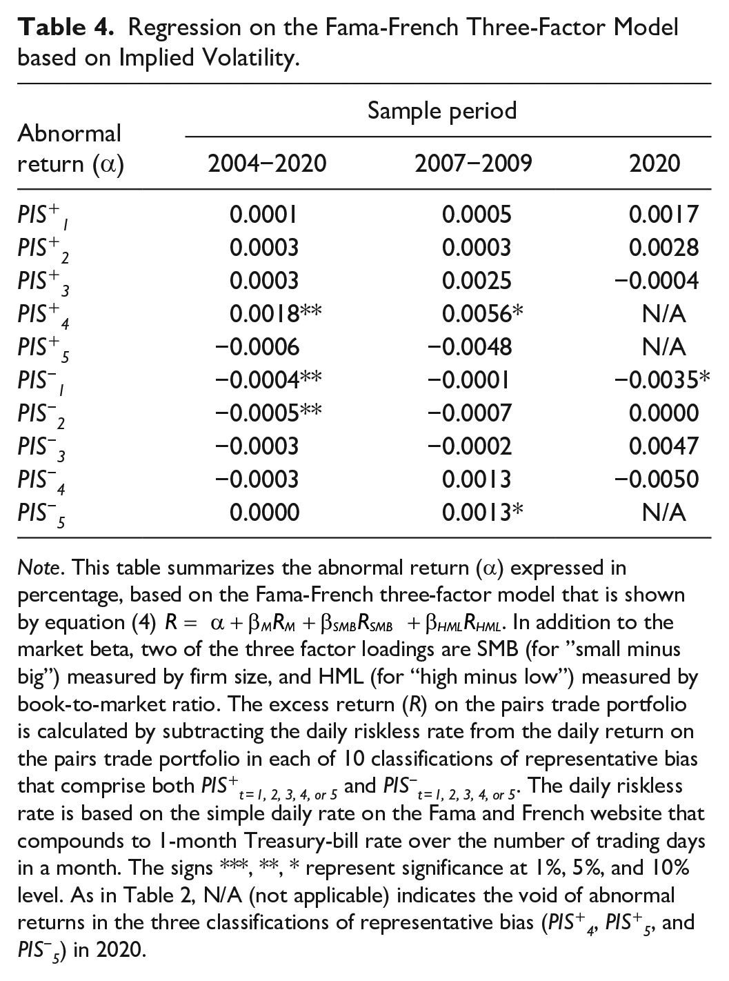
Note. This table summarizes the abnormal return (α) expressed in percentage, based on the Fama-French three-factor model that is shown by equation (4) $R = α + β_{M} R_{M} + β_{S M B} R_{S M B} + β_{H M L} R_{H M L}$ . In addition to the market beta, two of the three factor loadings are SMB (for ”small minus big”) measured by firm size, and HML (for “high minus low”) measured by book-to-market ratio. The excess return (R) on the pairs trade portfolio is calculated by subtracting the daily riskless rate from the daily return on the pairs trade portfolio in each of 10 classifications of representative bias that comprise both PIS⁺_{t = 1, 2, 3, 4, or 5} and PIS⁻_{t = 1, 2, 3, 4, or 5}. The daily riskless rate is based on the simple daily rate on the Fama and French website that compounds to 1-month Treasury-bill rate over the number of trading days in a month. The signs ***, **, * represent significance at 1%, 5%, and 10% level. As in Table 2, N/A (not applicable) indicates the void of abnormal returns in the three classifications of representative bias (PIS⁺₄, PIS⁺₅, and PIS⁻₅) in 2020.

Robustness Check

As a robustness check on implied volatilities in the options market mentioned in the previous section, conditional volatilities of GARCH models in the stock market are considered in this section because the sample is dealt with time-series data. For example, Sharma (2016) compares the conditional volatilities of 16 international stock indices by using a variety of GARCH methodologies. Following Bollerslev (1986), the simplest but very useful GARCH process is the GARCH(1, 1) process specified by the following three equations:

r_{t} = c + \emptyset_{1} r_{t - 1} + ε_{t}, ε_{t} = σ_{t} z_{t,} z_{t} ~ i . i . d . N (0, 1)

(5)

σ_{t}^{2} = w + α ε_{t - 1}^{2} + β σ_{t - 1}^{2}

(6)

L (μ, ω, α, β) = \frac{1}{v_{t} \sqrt{2 π}} e^{- \frac{ε_{t}^{2}}{2 v^{t}}}

(7)

where equation (5) models the conditional means and r_t that is the logarithmic return based on close-to-close price for each trading day [t − 1, t]. ε_t is the realized residual, defined as the difference between the actual return and long-run return (μ). Equation (6) is the conditional variance formula and σ_t² is the estimate of the latent conditional variance of the daily returns. Here, w, α, and β are the GRACH(1, 1) model parameters that maximize the sum of log-likelihood function, outlined by equation (7), under the assumption of the error term (z_t) being normally distributed.

Conditional volatilities are estimated according to equations (5), (6), and (7) using the daily close prices of iShares Russell 2000 ETF (IWM) and SPDR S&P 500 ETF (SPY) for the sample period of 2004 to 2020, and two subperiods in the same way as previous section defines. The daily logarithmic return (r_t) and conditional volatility (σ_t) can be easily computed through the maximum-likelihood estimation where the unconditional variance (w) is 0.000011, ARCH parameter (α) is 0.43, and GARCH parameter (β) is 0.57 in the GARCH(1, 1) specification. After calculating the time series of conditional volatilities of iShares Russell 2000 ETF (σ_t, Russell 2000) and SPDR S&P 500 ETF (σ_{t, S&P 500}), the OLS regression is used to estimate the degree of reaction of Russell 2000 investors, relative to S&P 500 investors, in the following equation:

\begin{array}{l} σ_{t, R u s s e l l 2000} = γ \times σ_{t, S & P 500} + {δ^{+}}_{1, C V} \times P I {S^{+}}_{1} \\ + {δ^{+}}_{2, C V} \times P I {S^{+}}_{2} + {δ^{+}}_{3, C V} \times P I {S^{+}}_{3} \\ + {δ^{+}}_{4, C V} \times P I {S^{+}}_{4} + {δ^{+}}_{5, C V} \times P I {S^{+}}_{5} \\ + {δ^{-}}_{1, C V} \times P I {S^{-}}_{1} + {δ^{-}}_{2, C V} \times P I {S^{-}}_{2} \\ + {δ^{-}}_{3, C V} \times P I {S^{-}}_{3} + {δ^{-}}_{4, C V} \times P I {S^{-}}_{4} \\ + {δ^{-}}_{5, C V} \times P I {S^{-}}_{5} \end{array}

(8)

where PIS⁺_t (PIS⁻_t) is a dummy variable for the upward (downward) movement of σ_{t, S&P 500} during the time interval t and the superscript + (−) represents the positive (negative) trend of σ_{t, S&P 500}. Specifically, PIS⁺_{t = 1, 2, 3, 4, or 5} (PIS⁻_{t = 1, 2, 3, 4, or 5}) will take on the value of one if σ_{t, S&P 500} sequentially moves upward (downward) in the previous 1, 2, 3, 4, or 5 trading days, and otherwise take on the value of zero. As the subscript CV stands for conditional volatility, the corresponding coefficients of PIS⁺_{t = 1 to 5} (PIS⁻_{t = 1 to 5}) are δ⁺_{t = 1 to 5, CV} (δ⁻_{t = 1 to 5, CV}) represent the scale of representative bias when Russell 2000 ETF investors perceive the increasing (decreasing) progression of the conditional volatilities of S&P 500 ETF investors in the past five trading days.

Table 5 presents the OLS regression results of conditional volatilities based on equation (8) above. Similar to the significance of β coefficient estimates in Table 2, the estimated slope coefficients (γ) of σ_{t, S&P 500} are statistically significant at the 1% significant level and imply that Russell 2000 ETF investors respond to the conditional volatility of S&P 500 ETF investors for the full sample period of 2004 to 2020 and two subperiods (2007–2009 and 2020). Regarding the estimates of the slope coefficients of previous information shock (PIS⁺_t or PIS⁻_t), δ⁺_{t = 1 to 5, CV} and δ⁻_{t = 1 to 5, CV}, are statistically significant for the whole sample period of 2004 to 2020, except for δ⁺_t = 4 and δ⁺_t = 5, indicating the evidence of representative bias of Russell 2000 ETF investors. One caveat is that the magnitude of representative bias, measured by δ⁺_{t = 1 to 5, CV} and δ⁻_{t = 1 to 5, CV}, is close to zero in the stock market and in line with the mixed evidence presented by De Bondt and Thaler (1985, 1987, 1990) and Fama (1998).

Table 5.

Regression Results of Conditional Volatility.

Coefficient	Sample period
Coefficient	2004−2020	2007−2009	2020
Γ	0.86***	0.77***	0.91***
δ ⁺ _{1, CV}	0.00***	0.00	0.00
δ ⁺ _{2, CV}	0.00***	0.00	0.00
δ ⁺ _{3, CV}	0.00**	0.00	0.00
δ ⁺ _{4, CV}	0.00	N/A	N/A
δ ⁺ _{5, CV}	0.00	N/A	N/A
δ ⁻ _{1, CV}	0.00***	0.00	0.00
δ ⁻ _{2, CV}	0.00***	0.00	0.00
δ ⁻ _{3, CV}	0.00***	0.00	0.00
δ ⁻ _{4, CV}	0.00***	0.00	0.00
δ ⁻ _{5, CV}	0.00**	0.00	0.00

Note. This table shows the results of equation (8) $\begin{array}{l} σ_{t, R u s s e l l 2000} = γ \times σ_{t, S & P 500} + {δ^{+}}_{1, C V} \times P I {S^{+}}_{1} + {δ^{+}}_{2, C V} \times P I {S^{+}}_{2} + {δ^{+}}_{3, C V} \\ \times P I {S^{+}}_{3} + {δ^{+}}_{4, C V} \times P I {S^{+}}_{4} + {δ^{+}}_{5, C V} \times P I {S^{+}}_{5} + {δ^{-}}_{1, C V} \times P I {S^{-}}_{1} + {δ^{-}}_{2, C V} \\ \times P I {S^{-}}_{2} + {δ^{-}}_{3, C V} \times P I {S^{-}}_{3} + {δ^{-}}_{4, C V} \times P I {S^{-}}_{4} + {δ^{-}}_{5, C V} \times P I {S^{-}}_{5}, \end{array}$ assuming that Russell 2000 investors respond to a series of public information embedded in the positive or negative tendency of the S&P 500 conditional volatility (σ_{t, S&P 500}). Russell 2000 conditional volatility (σ_t, Russell 2000) is regressed on both σ_{t, S&P 500} and previous information shock (PIS) where PIS⁺_t (PIS⁻_t) is a proxy for the upward (downward) movement of the S&P 500 conditional volatility during the time interval t and the superscript + (−) represents the positive (negative) trend of σ_{t, S&P 500}. For concreteness, PIS⁺_{t = 1, 2, 3, 4, or 5} (PIS⁻_{t = 1, 2, 3, 4, or 5}) will take on the value of one if S&P 500 conditional volatility moves upward (downward) in the previous 1, 2, 3, 4, or 5 trading days, respectively, and otherwise take on the value of zero. The signs ***, **, * represent significance at 1%, 5%, and 10% level. There are no observations pertaining to the upward progress of the S&P 500 conditional volatility over a window of 4 and 5 trading days (specifically, PIS⁺_{4, CV} and PIS⁺_{5, CV}) in the sub-periods of 2007 to 2009 and 2020; thus, N/A (not applicable) indicates missing coefficients of the two variables (PIS⁺₄ and PIS⁺₅) from 2007 to 2009 and in 2020.

During the first subperiod of 2007 to 2009 and second subperiod of 2020, all of the coefficient estimates of PIS⁺_{t = 1 to 5} and PIS⁻_{t = 1 to 5} (that is, δ⁺_{t = 1 to 5} and δ⁻_{t = 1 to 5}) are not statistically significant, meaning that Russell 2000 ETF investors are indifferent from previous information shock expressed in the consecutive 5-day conditional volatility in the S&P 500 ETF market. The findings of the two subperiods lend little support for representative bias probably because the two subperiods are characterized by economic disruptions that may dominate the effect of representative bias. Put differently, investors might pay more attention to economic conditions than representative bias in their decision-making process during a recession. In short, the results concerning the full sample period are consistent with well-established cognitive biases of S&P 500 traders (Cao et al., 2005; Poteshman, 2001) and resonate the excessive response hypothesis about the existence of representativeness between Russell 2000 and S&P 500 ETF traders.

There are some disparities between the results of Tables 2 and 5, except for the subperiod 2020. During the full sample period, the statistical significance of δ⁻_{t = 1 to 5} in Table 5 is contradicted with the statistical insignificance of δ⁻_{t = 1 to 5} in Table 2. During the subperiod of 2007 to 2009, the statistical insignificance of δ⁻_{t = 1 to 5} in Table 5 is opposed to the statistical significance of δ⁻_{t = 1 to 5} in Table 2. The diverged results between Tables 2 and 5 may raise because of the specification of models (Black–Scholes option pricing model vs. GARCH model) and the type of markets (stock market vs. options market). The results of Table 5 are based on the conditional volatility on stock markets; that is, the close prices of Russell 2000 and S&P 500 ETFs are the inputs to estimate conditional volatility in the GARCH (1, 1) model. On the other hand, the results of Table 2 are based on the implied volatility inferred from options market where the option price, stock price, risk-free interest rate, exercise price, and time to expiration are the inputs to estimate implied volatility in the Black–Scholes option pricing model.

Table 6 summarizes the abnormal return (α) of the Fama and French three-factor model, outlined in equation (4). Not reported here, the daily returns of three simple trading mechanisms (long position on the S&P 500 index, short position on the Russell 2000 index, and pairs trade portfolio) are calculated in the same way as those in Table 3, with the exception of using the movement of conditional volatility as the criteria of representativeness. Then, the time series of the excess return (R) of the pairs trade portfolio is formed by subtracting the daily riskless rate from the daily return of the pairs trade portfolio when the criteria of representative bias are met; namely, the respective PIS⁺ or PIS⁻ variables are registered as the value of one when S&P 500 conditional volatility consecutively ascends (descends) during the preceding 1, 2, 3, 4, or 5 trading days. The Fama and French three-factor model regresses the excess return (R) against market index (R_M), firm size (R_SMB), and book-to-market ratio (R_HML) factors. The majority of abnormal returns in Table 6 are close to zero and statistically insignificant, except for PIS⁻₁ and PIS⁻₃ in the 2004 to 2020 full sample period, PIS⁺₃ in the 2007 to 2009 subperiod, and PIS⁻₂ and PIS⁻₃ in 2020. Quantitatively similar to those of Table 4, the empirical results of Table 6 are in opposition to sensitivity to information hypothesis, and in favor of the market efficiency hypothesis that pairs trade portfolio using the representative bias of the conditional volatility cannot offer riskless returns.

Table 6.

Regression on the Fama-French Three-Factor Model Based on Conditional Volatility.

Abnormal return (α)	Sample period
Abnormal return (α)	2004−2020	2007−2009	2020
PIS ⁺ ₁	0.0000	0.0007	0.0034
PIS ⁺ ₂	0.0000	−0.0034	0.0168**
PIS ⁺ ₃	−0.0016	−0.0200**	0.0189
PIS ⁺ ₄	−0.0007	N/A	N/A
PIS ⁺ ₅	0.0145	N/A	N/A
PIS ⁻ ₁	−0.0006**	−0.0001	−0.0029
PIS ⁻ ₂	−0.0005	0.0006	−0.0049
PIS ⁻ ₃	−0.0008*	−0.0005	−0.0088**
PIS ⁻ ₄	−0.0004	0.0006	−0.0115
PIS ⁻ ₅	−0.0008	−0.0010	−0.0099

Note. This table summarizes the abnormal return (α) expressed in percentage, based on the Fama-French three-factor model that is shown by equation (4) $R = α + β_{M} R_{M} + β_{S M B} R_{S M B} + β_{H M L} R_{H M L}$ . In addition to the market beta, two of the three factor loadings are SMB (for “small minus big”) measured by firm size, and HML (for “high minus low”) measured by book-to-market ratio. The excess return (R) on the pairs trade portfolio is calculated by subtracting the daily riskless rate from the daily return on the pairs trade portfolio in each of 10 classifications of representative bias that comprise both PIS⁺_{t = 1, 2, 3, 4, or 5} and PIS⁻_{t = 1, 2, 3, 4, or 5}. The daily riskless rate is based on the simple daily rate on the Fama and French website that compounds to 1-month Treasury-bill rate over the number of trading days in a month. The signs ***, **, * represent significance at 1%, 5%, and 10% level. As in Table 5, N/A (not applicable) indicates the void of abnormal returns in the two classifications of representative bias (PIS⁺₄ and PIS⁺₅) from 2007 to 2009 and in 2020.

Implications and Limitations

The findings of this study have four practical implications. First, the findings offer handful information of both the implied and conditional volatilities of both S&P 500 and Russell 2000 indexes to day traders, arbitragers, and portfolio managers. Practitioners may forecast investor reaction to new information contained in the trend of implied and conditional volatilities in the options and stock markets, respectively, under the assumption that investors subscribe to some degree of representativeness. Second, investor misreaction is slightly prevalent in both options and stock markets; that is, both options and ETF investors tend to misreact, but may underreact/overact in different way. Third, a simple trading strategy of pairs trade based on representative bias is no guarantee of investment outcomes, even in the absence of transaction costs. An important question for future research is to develop a profitable trading strategy that credibly accounts for transactions costs in the options and stock markets. Promising avenues of research may focus on exploring the adaptation of asymmetrical representativeness over time and devising sophisticated trading algorithms that take advantage of the riskless arbitrage, if any, as a result of the asymmetrical representativeness heuristic. Fourth, future work can examine the representative bias, if any, between different types of investors, that is, value versus growth investors, instead of small- versus large-cap investors in this study. The value portfolio can be proxied by the Dow Jones Industrial Average (DJIA) index that tracks 30 large, publicly-owned blue-chip companies, while the growth portfolio can be proxied by the NASDAQ composite index that is the market capitalization-weighted index of over 3,000 common equities listed on the Nasdaq stock exchange.

There are fourth limitations in this research. First, this article does not address why the property of asymmetrical representativeness of Russell 2000 options investors alters over time, that is, the coefficients δ⁺ and δ⁻ invert from negative in the 2004 to 2020 sample period to positive between 2007 and 2009, as shown in Table 2. Second, the findings of this study cannot explain the Russell 2000 options investors’ insensitivity to representative bias in 2020, in light of the severe economic impact of the coronavirus outbreak. Likewise, this article cannot explain why Russell 2000 ETF traders do not subscribe to representativeness in the first subperiod of 2007 to 2009 and the second subperiod of 2020, using conditional volatilities, as shown in Table 5. Third, the implied volatility in the Black−Scholes options pricing model can be misestimated. Alternatively, a variety of presumed stochastic volatility models can be employed as the model of options market equilibrium for the purpose of representativeness tests, such as the Heston (1993) model that incorporates a nonzero market price of variance risk; namely, instantaneous volatility as opposed to implied volatility in the Black−Scholes model. Forth, the basic GARCH models have been extended in many ways and are especially suited to estimate the conditional volatility of financial instruments. For example, the threshold-GARCH (TGARCH) and exponential-GARCH (EGARCH) models allow for the asymmetric effects of volatility shocks; that is, negative shocks to behave differently than positive shocks, assuming that negative news has a more prominent effect on the volatility of asset prices than does good news. One can also include macroeconomic explanatory variables, that is, unemployment rate, GDP, and inflation, in the equations of TGARCH and EGARCH models for estimating the conditional volatility.

Conclusions

Implied volatility and conditional volatility are a measure of risk and a proxy for the misreaction of traders in the options and stock markets, respectively. Comparing the reactions between Russell 2000 and S&P 500 investors in the options market reduces, to some extent, the methodology problem and measurement error as a result of time-varying risk premiums in the stock markets. The estimation results of regressing IVRussell 2000 against the trend of S&P 500 implied volatility serving as a reference for representativeness suggest that Russell 2000 options investors are not receptive to representative bias, in spite of inconclusive evidence for asymmetrical responsiveness. For the 2004 to 2020 sample period, IVRussell 2000 declines when the trend of S&P 500 implied volatility ascends within five trading days, other things being equal. During the 2008 global financial crisis, IVRussell 2000 elevates when the trend of S&P 500 implied volatility descends within five trading days. Traders seem to exhibit complex behavior in dealing with options and equity securities, and forthcoming research could scrutinize why the property of asymmetrical representativeness in the options market is time-dependent and event-driven.

As a robustness check on the representative bias from the viewpoint of implied volatilities in the options market, conditional volatilities are estimated based on GARCH (1, 1) model using the iShares Russell 2000 and SPDR S&P 500 ETFs. For the full example period of 2004 to 2020 shown in Table 5, it appears that Russell 2000 ETF traders adjust upwards their expectations of conditional volatilities after observing a trend of mostly increasing or decreasing conditional volatilities in the S&P 500 ETF; namely, Russell 2000 ETF traders tends to overact and increase their expectation of risk, relative to S&P 500 ETF traders. The overaction of Russell 2000 ETF traders might be explained by the fact that Russell 2000 ETF which is a proxy of small firms is considered riskier than S&P 500 ETF which is a proxy of large firms. However, there is no evidence of the overaction of Russell 2000 ETF traders in the two subperiods. Future research can inspect why such overreaction dissipated in times of market turmoil. One plausible reason is that Russell 2000 ETF traders are influenced more by other market-wide concerns (i.e., the ripple effect of the mortgage market on the stock market from 2007 to 2009 and COVID-19 pandemic in 2020) than the representative bias. Regardless of utilizing the time series of implied volatilities and conditional volatilities, the empirical results of Fama-French Three-Factor Model rejects the sensitivity to information hypothesis in both options and stock markets, owing to trivial abnormal return.

This article fills the gap in the related literature by comparing Russell 2000 and S&P 500 investors since most of the literature examine the representative bias by one type of investors (e.g., S&P 500 investors). Furthermore, past studies do not explore the relationship between the representative bias and abnormal return from the perspective of both conditional and implied volatilities. This paper contributes to the understanding of representativeness by providing weak evidence on asymmetrical representativeness in the options market, and somewhat evidence on representativeness in the stock market. However, such behavioral partiality does not end up with arbitrage profits in the stock market because of insignificant abnormal returns according to the Fama and French three-factor model. One caveat is that the magnitude of misreaction conditional on representativeness may be too small to inflate the stock price and to reward arbitrageurs before the trading price converges to its rational level. The limited existence of asymmetrical representative bias in conjunction with the void of abnormal returns implies complicated traits of investors. In light of annulled representativeness and abnormal return, the overall results concerning the linkage between representative bias and successful pairs trading strategies conforms to the efficient markets hypothesis.

Footnotes

Acknowledgements

The author would like to thank the editor and three anonymous referees for their very helpful suggestions. All remaining errors are my own.

Declaration of Conflicting Interests

The author declared no potential conflicts of interest with respect to the research, authorship, and/or publication of this article.

Funding

The author received no financial support for the research, authorship, and/or publication of this article.

ORCID iD

Yen-Sheng Lee

References

Abdin

Farooq

Sultana

Farooq

(2017). The impact of heuristics on investment decision and performance: Exploring multiple mediation mechanisms. Research in International Business and Finance, 42, 674–688.

Baglioni

Monticini

(2010). The intraday interest rate under a liquidity crisis: The case of August 2007. Economics Letters, 107, 198–200.

Baker

H. K.

Kumar

Goyal

Gaur

(2019). How financial literacy and demographic variables relate to behavioral biases. Managerial Finance, 45, 124–146.

Berk

Green

Naik

(1999). Optimal investment, growth options, and security returns. Journal of Finance, 54, 1553–1607.

Bhandari

L. C.

(1988), Debt/equity ratio and expected common stock returns: Empirical evidence. Journal of Finance, 43, 507–528.

Black

Scholes

(1973). The pricing of options and corporate liabilities. Journal of Political Economy, 81, 637–654.

Bollerslev

(1986). Generalized autoregressive conditional heteroskedasticity. Journal of Econometrics, 31, 307–327.

Bordalo

Gennaioli

La Porta

Shleifer

(2019). Diagnostic expectations and stock returns. Journal of Finance, 74, 2839–2874.

Cao

(2005). Is investor misreaction economically significant? Evidence from short- and long-term S&P 500 index options? The Journal of Futures Markets, 25, 717–752.

10.

Chaudhuri

T. D.

Ghosh

Singh

(2017). Application of machine learning tools in predictive modeling of pairs trade in Indian Stock Market. IUP Journal of Applied Finance, 23, 5–25.

11.

Clegg

Krauss

(2018). Pairs trading with partial cointegration. Quantitative Finance, 18, 121–138.

12.

De Bondt

Thaler

. (1985). Does the stock market overreact? Journal of Finance, 40, 793–805.

13.

De Bondt

Thaler

. (1987). Further evidence on investor overreaction and stock market seasonality. Journal of Finance, 42, 557–581.

14.

De Bondt

Thaler

. (1990). Does security analysts overreact? American Economic Review, 80, 52–57.

15.

Dickey

Fuller

(1981). Likelihood ratio statistics for autoregressive time series with a unit root. Econometrica, 49, 1057–1072.

16.

Diz

Finucane

(1993). Do the options markets really overreact? The Journal of Futures Markets, 13, 299–312.

17.

Faff

(2010). Does simple pairs trading still work? Financial Analysts Journal, 66, 83–95.

18.

Fama

(1998). Market efficiency, long-term returns, and behavioral finance. Journal of Financial Economics, 49, 283–306.

19.

Fama

French

(1992). The cross-section of expected stock returns. Journal of Finance, 47, 427–466.

20.

Fama

French

(1996). Multifactor explanations of asset pricing anomalies. Journal of Finance, 51, 55–84.

21.

Fama

French

(2004). The capital asset pricing model: Theory and evidence. Journal of Economic Perspective, 18, 25–46.

22.

Farago

Hjalmarsson

(2019). Stock price co-movement and the foundations of pairs trading. Journal of Financial and Quantitative Analysis, 54, 629–665.

23.

Flannery

Kwan

Nimalendran

(2013). The 2007–2009 financial crisis and bank opaqueness. Journal of Financial Intermediation, 22, 55–84.

24.

Garivaltis

(2019). Super-replication of the best pairs trade in hindsight. Cogent Economics & Finance, 7, 1–14.

25.

Goetzmann

Massa

(2002). Daily momentum and contrarian behavior of index fund investors. Journal of Financial and Quantitative Analysis, 37, 375–389.

26.

Goldkamp

Dehghanimohammadabadi

(2019). Evolutionary multi-objective optimization for multivariate pairs trading. Expert Systems with Applications, 135, 113–128.

27.

Harvey

Whaley

(1992). Market volatility prediction and the efficiency of the S&P 100 index option market. Journal of Financial Economics, 31, 43–74.

28.

Heston

S. L.

(1993). A closed-form solution for options with stochastic volatility with applications to bond and currency options. Review of Financial Studies, 6, 32.

29.

Hibbert

Daigler

Dupoyet

(2008). A behavioral explanation for the negative asymmetric return-volatility relation. Journal of Banking and Finance, 32, 2254–2266.

30.

Hong

Stein

(1999). A unified theory of underreaction, momentum trading, and overreactions in asset markets. Journal of Finance, 54, 2143–2184.

31.

Huang

Martin

(2019). Pairs trading strategies in a cointegration framework: Back-tested on CFD and optimized by profit factor. Applied Economics, 51, 2436–2452.

32.

Isidore

R. R.

Christie

(2019). Model to predict the actual annual return of the investor with the investors’ behavioral biases as the independent variables. Journal of Private Equity, 22, 70–82.

33.

Ivanov

Jones

Zaima

J. K.

(2013). Analysis of DJIA, S&P 500, S&P 400, NASDAQ 100 and Russell 2000 ETFs and their influence on price discovery. Global Finance Journal, 24, 171–187.

34.

Javed

Bagh

Razzaq

(2017). Herding effects, over confidence, availability bias and representativeness as behavioral determinants of perceived investment performance: An empirical evidence from Pakistan Stock Exchange (PSX). Journal of Global Economics, 6, 1–13.

35.

Kahneman

Tversky

(1973). Subjective probability: A judgment of representativeness. Cognitive Psychology, 3, 430–454.

36.

Kanojia

Singh

Goswami

(2018). An empirical analysis of the factors influencing individual investors. IOSR Journal of Business and Management, 20, 30–37.

37.

La Porta

Lakonishok

Shleifer

Vishny

. (1997). Good news for value stocks: Further evidence on market efficiency. Journal of Finance, 52, 859–874.

38.

Lakonishok

Shleifer

Vishny

(1994). Contrarian investment, extrapolation, and risk. Journal of Finance, 49, 1541–1578.

39.

Law

K. F.

W. K.

L. H.

(2018). A single-stage approach for cointegration-based pairs trading. Finance Research Letters, 26, 177–184.

40.

Lintilhac

P. S.

Tourin

(2017). Model-based pairs trading in the bitcoin markets. Quantitative Finance, 17, 703–716.

41.

Liu

Chang

L. B.

Geman

(2017). Intraday pairs trading strategies on high frequency data: The case of oil companies. Quantitative Finance, 17, 87–100.

42.

Poteshman

(2001). Underreaction, overreaction, and increasing misreaction to information in the options markets. Journal of Finance, 56, 851–876.

43.

Rad

Low

Faff

(2016). The profitability of pairs trading strategies: Distance, cointegration and copula methods. Quantitative Finance, 16, 1541–1558.

44.

Rasheed

M. H.

Rafique

Zahid

Akhtar

M. W.

(2018). Factors influencing investor’s decision making in Pakistan: Moderating the role of locus of control. Review of Behavioral Finance, 10, 70–87.

45.

Roll

(1977). A critique of the asset pricing theory"’s tests. Journal of Financial Economics, 4, 129–176.

46.

Rozeff

Zaman

(1998). Overreaction and insider trading: Evidence from growth and value portfolios. Journal of Finance, 53, 701–716.

47.

Shah

S. Z. A.

Ahmad

Mahmood

(2018). Heuristic biases in investment decision-making and perceived market efficiency: A survey at the Pakistan stock exchange. Qualitative Research in Financial Markets, 10, 85–110.

48.

Shankar

(2007). Active versus passive index management: A performance comparison of the S&P and the Russell indexes. The Journal of Investing, 16, 85–95.

49.

Sharma

(2016). Forecasting stock market volatility using Realized GARCH model: International evidence. The Quarterly Review of Economics and Finance, 59, 222–230.

50.

Sharpe

W. F.

(1964). Capital asset prices: A theory of market equilibrium under conditions of risk. Journal of Finance, 19, 425–442.

51.

Smith

R. T.

(2017). A good pair: Alternative pairs-trading strategies. Financial Markets and Portfolio Management, 31, 1–26.

52.

Stein

(1989). Overreactions in the options market. Journal of Finance, 44, 1011–1024.

53.

Stübinger

Endres

(2018). Pairs trading with a mean-reverting jump–diffusion model on high-frequency data. Quantitative Finance, 418, 1735–1751.

54.

Tie

Zhang

(2018). An optimal strategy for pairs trading under geometric brownian motions. Journal of Optimization Theory and Applications, 179, 654–675.

Representative Bias and Pairs Trade: Evidence From S&P 500 and Russell 2000 Indexes

Abstract

Keywords

Introduction

Literature Review

Hypotheses

Methodology

Data and Regrssion Results

Robustness Check

Implications and Limitations

Conclusions

Footnotes

Acknowledgements

Declaration of Conflicting Interests

Funding

ORCID iD

References