Sage Journals: Discover world-class research

Abstract

STEN (Standard Ten) is the most frequently preferred score generating method among the norm reference scores (e.g., percentile rank, STANINE) However, it is usually misleading because of the skewness presented with the data. In this study, rather than STEN, GRiSTEN (Golden Ratio in Statistics) approach is proposed to generate relatively fair outcomes. The GRiSTEN method acknowledges the effects of skewness by accounting for the contribution of each data element to the center point based on its specific location in the data stack. Generating norms using the GRiSTEN approach enables us to mark “the most capable” or “the least capable” scores regarding the test without involving too many arithmetic operations. In order to verify the applicability of the psychometric tests based on System Sigma run by Mevasis IT Consultancy in Turkey, a watch test, which is designed to observe respondents’ estimation of velocity, is carried out with a pilot group consisting of 407 male respondents aged between 30 and 50. By using GRiSTEN approach, it is shown that consistent outputs can be obtained without changing, ignoring, or transforming any elements regardless of the number of elements, skewness, distribution, and values of the data array.

Keywords

skewness norm-referenced scores psychometrics GRiSTEN score STEN score STANİNE percentile rank

Introduction

Numerous behavioral assessments (Shea et al., 2014) rely heavily on normative samples to make comparisons between people. A group of scores from the respondents assessed is obtained and then compared with each respondent’s score to form a normative sample or norm (Reznick, 1989).

This norm provides a context, that is, an established frame of reference, allowing for a meaningful interpretation of the results. Raw scores obtained from normative samples can be turned into percentile ranks with a conversion table, which offers a researcher two options, that is, raw scores or percentile ranks, in a statistical analysis. The percentile rank in respect to the raw score technique mentioned here is developed due to the skewness appearing in the real data (Bornmann, 2013). However, it has some shortcomings to be considered by test users (Thompson, 1993). The first most important of these flaws is that the norm referenced percentile ranks are not clear. The highest could be taken as either 5% or 10%, depending on the analyst’s choice. The second most important flaw is that norm score ranges are variable.

Consequently, small raw score differences are associated with large percentile differences at the center of the distribution. On the contrary, large raw score differences are associated with small percentile differences at the extremes of the distribution. (Brown, 1976). The raw scores between 51 and 87 may indicate the top score 10, but the raw scores between 42 and 50 may indicate 9. However, conversion of the raw scores into percentile ranks results in a change in the distribution pattern and cannot maintain the difference between scale units (Crocker & Algina, 1986). Moreover, arithmetic operations such as addition, subtraction, or multiplication cannot be applied to percentile ranks (Rodriguez, 1997). Thus, statisticians hesitate to make use of raw scores with respect to percentile ranks and opt for parametric approaches such as STEN in general.

The indicator of a respondent’s relative position as a range of values in context of the population is a STEN score (Canfield, 1951). STEN scores divide a score scale into 10 units, with STEN 2, 3, 4, 5, 6, 7, 8, and 9 covering a range of a one-half standard deviation (0.5σ) for each, and STEN 1 and 10 covering the remaining scores in the left and right tail, respectively. In other words, when STEN scores are used, most of the respondents fall into the average range making about 2% of them fall into the outliers of 1 or 10 in the Bell curve. Individual STEN scores are defined in reference to a standard normal distribution (see Figure 1; Coaley, 2010).

Figure 1.

The comparison of norm-referenced scores and their relationship with the normal distribution.

The midpoint of STEN scoring system is the value 5.5. The STEN scoring system is normally distributed and then divided into 10 parts by letting 0.5 standard deviations correspond to each point of the scale. The STEN scores are demarcated by −2, −1.5, −1, −0.5, 0, 0.5, 1, 1.5, and 2.0.

Each of these numbers can be assumed as z-scores in the standard normal distribution. The remaining tails of the distribution are equivalent to the 1st and 10th STEN scores. So less than −2 corresponds to a score of 1, and greater than 2 corresponds to a score of 10. STANINE and t score are the transformed z scores like STEN. STANİNE score is divided into nine points and produces a normal distribution whose mean is 5, and whose standard deviation is 1 (Clark-Carter, 2005). T score produces a normal distribution whose standard deviation is 10 and whose mean is 50 (Coaley, 2010).

Despite being commonly preferred, STEN has some drawbacks. It is based on standard scoring principles and makes one think within score ranges rather than absolute scores. The ranges formed with STEN are not sufficient to indicate important differences among respondents. In addition, the analysts cannot interpret the minute differences between the scores as required. Another limitation of STEN scoring is that it presents scores by processing non-normally distributed data as if it were distributed normally. Skewness is of great of importance here. It refers to a lack of symmetry in data distribution. The values are concentrated in the left or right tail. Every data array does not show normal distribution in nature. Thus, it does not have to be symmetrical. It can be positively or negatively skewed. Therefore, skewness plays an important role in obtaining significant outputs. However, scaling approaches like STEN neither take these outliers stemming from skewness into consideration nor yield a symmetrical distribution curve.

Outliers that “skew” (Doane & Seward, 2011) the mean either up or down will overstate one side of the average and understate the other. Therefore, the number of scores above and below the mean value should be approximately equivalent. Exclusion of data (Pleace, 2016) from the sample results in a higher or lower mean. Another consequence of data exclusion is the perception of scores. They may be perceived as below or above the mean when the opposite is true. The spread of results appears narrower, offering a smaller apparent standard deviation with the culling of data (Tummaruk et al., 2009) from one or both ends of the distribution. Accordingly, a respondent’s scores may appear further from the mean and more extreme than they actually are.

False “floor-effects” (Whitaker & Wood, 2008) are introduced with the exclusion of usually low scores, which serve to “unbalance” the distribution. A resulting positive skewness:

Overstates the scores of those below the true mean

Understates the scores of those above the true mean

Yields inordinate scores in the mean range (within 1 standard deviation of the mean)

The normal distribution function has been most frequently used in assessing continuous data, which is not commonly observed in nature (Pearson, 1920). This raises concerns since a lot of the observable data around us tends to be skewed. Misleading effects of skewness can be dealt with by the GRiSTEN (Golden Ratio In Statistics; Gunver et al., 2018) method, which considers the contribution of each data element to the center point as well as its specific location in the data stack. STEN explains negative and positive skewness with a single parameter, whereas GRiSTEN shows it with two different parameters. To illustrate, the former makes the output stretch by 5 units in both tails while the latter makes it stretch by 7 units in the right tail and by 3 units in the left tail. Thus, GRiSTEN can overcome skewness by differentiating the parameters in right and left tails.

There are deficiencies in norm scoring assessment in skewed data. Can a different method of norm scoring assessment be tried on skewed data and give a better result? Could GRIS, which was previously developed by Gunver et al. (2018), be an alternative in this regard?

The aim of this study is to evaluate STEN, which is a standard method for norm score assessment, and GRISTEN, a new method, in skewed data.

Materials and Methods

Materials

A pilot study was carried out to validate Turkish psychometric tests conducted by Mevasis Bilisim Danismanlik (Mevasis | HPC Çözüm Ortağı, 2015), which are developed with System Sigma (Alfa-electronics, 2018). Snowball sampling method was used for sampling. Web site Public announcment by Mevasis Bilisim Danismanlik was applied (Mevasis | HPC Çözüm Ortağı, 2015). All people who wanted to participate were included in the sample. A total of 407 male respondents aged 30 to 50 are included in a Watch test. All respondents were provided written consent prior to having the tests.

The watch test is a psychometric test which aims to define velocity-distance abilities. By measuring the reaction time, the watch test aims to show how precise a respondent can be when they react to an event and whether they can demonstrate their reaction with or without creating a time lag.

The vane moves toward 12 with a constant velocity and disappears at a specified point keeping its move hidden. The respondent is asked to hit 12 when he assumes the vane has arrived at 12. There are three selections of velocity and each are repeated six times (see Figure 2).

Figure 2.

Watch test. In the watch test, there is a screen displaying a clock and a stop button. The respondent is asked to tap the button on the screen when he assumes that the vane has hit 12.

Low velocity watch test: The velocity of vane is 6.25°/s. In the low velocity Watch test, the vane appears at 11:45 and disappears at 11:53. The respondent is expected to estimate the velocity of the vane from the moment it appears until it disappears, and by taking the velocity into account, to respond to it when he assumes it is 12 sharp.

Medium velocity watch test: The velocity of vane is 8°/s. In the medium velocity watch test, the vane appears at 11:40 and disappears at 11:50. The respondent is expected to estimate the velocity of the vane from the moment it appears until it disappears, and by taking the velocity into account, to respond to it when he assumes it is 12 sharp.

High velocity watch test: The velocity of vane is 16.6°/s In the high velocity watch test, the vane appears at 11:20 and disappears at 11:40. The respondent is expected to estimate the velocity of the vane from the moment it appears until it disappears, and by taking the velocity into account, to respond to it when he assumes it is 12 sharp.

All time lags in six tests for each respondent are tallied up to form the respondent’s total score, which is called “a performance score.” If the respondent fails to hit 12 on any event, absolute time lag is set to 1,500 ms. The watch performance score is the average of low, medium, and high velocity performance scores. Short time lags are defined as high norm scores while high performance scores refer to low norm scores.

The histograms of these scores, which are developed by Percentile bin (Pb) method (Gunver et al., 2017) are given below. Standard deviation is taken into account to create the histogram divisions according to Scott’s normal reference rules. However, the standard deviation is unnecessarily large, especially with skewed data. Therefore, an alternative method is proposed to create histograms. The narrowest area containing 4% of the data stack is sought. It is expected to be around the median, especially in symmetrical data heaps. The reason why the percentiles are increased by four is it is the smallest divider that divides 100 but not 50. If the data stack contains more than 4% repeating members in time, the Sequential Difference (SeDi) can be zero. However, since the histogram bin cannot be equal to zero, a correction column is set up, and when the percentiles are increased by four at a time, all zeros are replaced by the maximum consecutive difference between percentiles. When the percentiles are increased by four at a time, the narrowest distance greater than zero is determined as the histogram division ( $\overset{\land}{h}$ ). This new method is called Percentile bin (Pb). In the histogram graphs (Figures 3 –6) obtained through the Pb method, the horizontal axis shows the time lag in milliseconds, and the vertical axis shows the number of people with that time lag.

Figure 3.

Low velocity watch test.

Figure 4.

Medium velocity watch test.

Figure 5.

High velocity watch test.

Figure 6.

Watch performance score.

Methods

The performance scores of the mentioned tests are converted to both STEN scores and GRiSTEN scores. The GRiSTEN scores are calculated based on the approach of GRIS. (Gunver et al., 2018) due to the skewness of the scores. This approach proposes calculations of G (coefficient of skewness), O (GRiSTEN mean), and DLeft and DRight (GRiSTEN deviations), which are performed with a Matlab code (GRiS Matlab, 2018). A calculator (Goldenratioinstatistics.com., 2020) has been developed so that these calculations can be made easily by the users.

Coefficient of skewness (G): “In addition to the other skewness measurement formulas, the coefficient of skewness allows calculating the skewness independently of the sample size.

G = \frac{f o r a l l x_{i} < m e d \Rightarrow \sum (x_{i} - m e d)}{e l s e \Rightarrow \sum (x_{i} - m e d)}

GRiSTEN mean (O): A linear new mean (O), which takes the large value of the golden ratio in the median and the small value of the golden ratio at the outliers, is designed.

GRiSTEN Deviations (DLeft and DRight): The most remarkable point about GRiSTEN deviation is that it allows calculating two independent deviations for each side of the GRiSTEN Mean.

The calculations are presented in Table 1.

Table 1.

Calculation of the Scores Presented by STEN and GRiSTEN.

Norm Score	STEN	GRiSTEN
1	Score ≥ $\bar{x}$ + 2 s	Score ≥ O + 2 DRight
2	+ 2 s > Score ≥ $\bar{x}$ + 1.5 s	O + 2 DRight > Score ≥ O + 1.5 DRight
3	$\bar{x}$ + 1.5 s > Score ≥ $\bar{x}$ + s	O + 1.5 DRight > Score ≥ O + DRight
4	$\bar{x}$ + s > Score ≥ $\bar{x}$ + 0.5 s	O + DRight > Score ≥ O + 0.5 DRight
5	$\bar{x}$ + 0.5 s > Score ≥ $\bar{x}$	O + 0.5 DRight > Score ≥ O
6	$\bar{x}$ > Score ≥ $\bar{x}$ − 0.5 s	O > Score ≥ O + 0.5 DLeft
7	$\bar{x}$ − 0.5 s > Score ≥ $\bar{x}$ − s	O + 0.5 DLeft > Score ≥ O + DLeft
8	$\bar{x}$ − s > Score ≥ $\bar{x}$ − 1.5 s	O + DLeft > Score ≥ O + 1.5 DLeft
9	$\bar{x}$ − 1.5 s > Score ≥ $\bar{x}$ − 2 s	O + 1.5 DLeft > Score ≥ O + 2 DLeft
10	$\bar{x}$ − 2 s > Score	O + 2 DLeft > Score

Note. $\bar{x}$ = arithmetic mean; s = standard deviation; O = GRiSTEN mean; DLeft = left-skewed distribution; DRight = right-skewed distribution.

Table 1 shows the scores that STEN and GRiSTEN present in certain cases. For example; if the respondent’s score is greater than the sum of $\bar{x}$ (mean) and 2 s (two standard deviations), STEN presents a norm score of 1. Similarly, if the respondent’s score is greater than the sum of O (GRiSTEN mean) and 2DRight (skewed to the right by 2 units), GRiSTEN presents 1 as the norm score.

Results

The low velocity watch test (Figure 3), medium velocity watch test (Figure 4), and high velocity watch test (Figure 5) graphics are created by transforming the total time lags produced by the respondent into norm reference scores. The watch performance score graph (Figure 6) is created according to the total number of time lags produced by the respondent.

As this study is focused on skewness, which causes misleading results, Table 2 demonstrates the effects of skewness on the descriptives.

Table 2.

Descriptives.

	Low velocity watch test	Medium velocity watch test	High velocity watch test	Watch performance score
Min	293.00	160.00	170.00	267.67
Max	4,747.00	6,480.00	6,020.00	5,439.00
Q1	1,093.00	600.00	710.00	926.67
Median	1,680.00	980.00	1,200.00	1,316.67
Q3	2,347.00	1,560.00	1,970.00	1,996.67
Arithmetic mean ( $\bar{x}$ )	1,816.96	1,231.10	1,511.74	1,519.93
Standard deviation (s)	944.44	919.77	1,116.11	846.15
G₁	0.75	1.98	1.40	1.26
G	−0.69	−0.43	−0.44	−0.52
O	1,774.45	1,155.56	1,421.06	1,465.81
Dright	1,058.61	1,090.09	1,403.14	1,035.81
Dleft	−747.24	−545.07	−705.95	−578.87

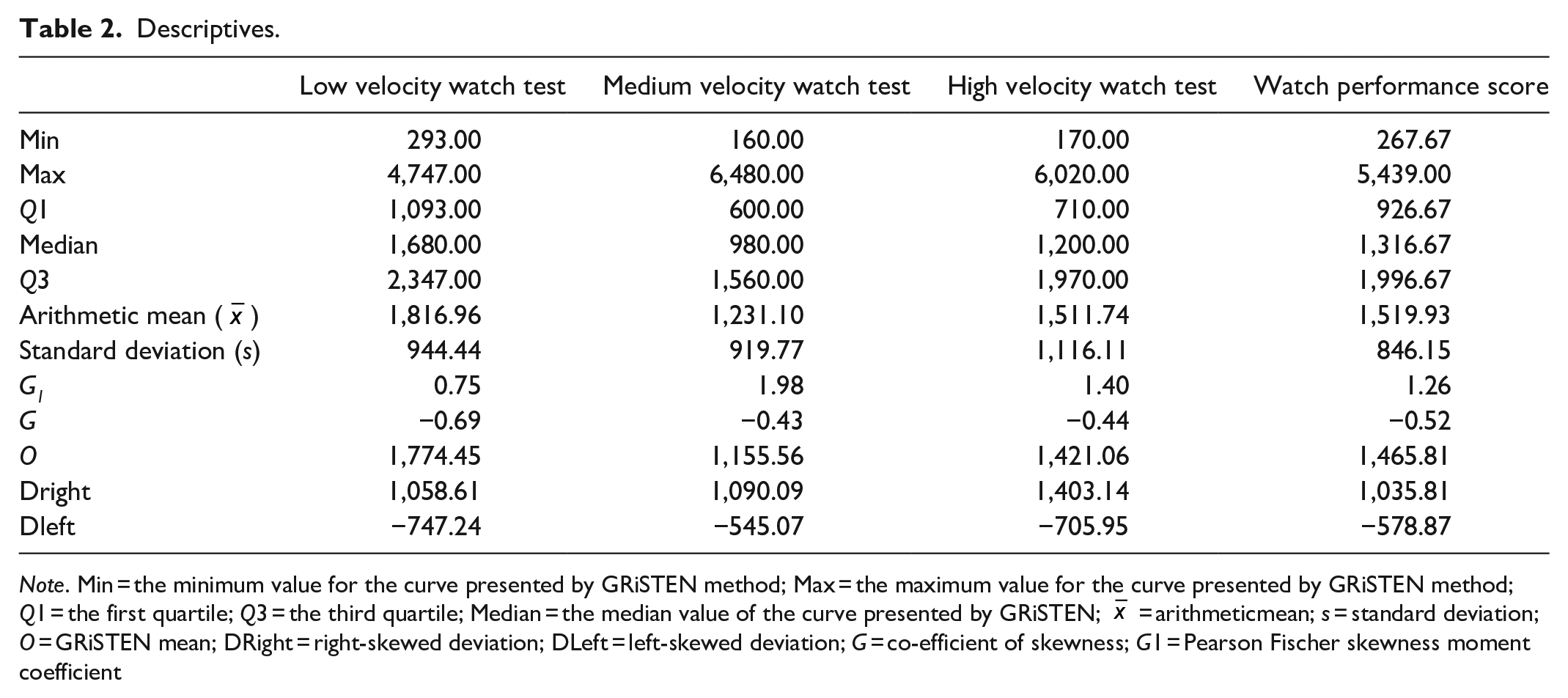
Note. Min = the minimum value for the curve presented by GRiSTEN method; Max = the maximum value for the curve presented by GRiSTEN method; Q1 = the first quartile; Q3 = the third quartile; Median = the median value of the curve presented by GRiSTEN; $\bar{x}$ = arithmetic mean; s = standard deviation; O = GRiSTEN mean; DRight = right-skewed deviation; DLeft = left-skewed deviation; G = co-efficient of skewness; G1 = Pearson Fischer skewness moment coefficient

In Table 2, G and G1 show that the distribution is not normal. Considering these values, it can be inferred that GRiSTEN should be used in non-normal distribution.

The scores of STEN, which overlooks skewness, and the scores of GRiSTEN, which takes skewness into account, are presented in Table 3.

Table 3.

STEN and GRiSTEN Scores.

	Watch performance score		High velocity watch test		Medium velocity watch test		Low velocity watch test
	GRiSTEN	STEN	GRiSTEN	STEN	GRiSTEN	STEN	GRiSTEN	STEN
1	@ ≥ 3,153	@ ≥ 3,212	@ ≥ 4,227	@ > 3,744	@ > 3,336	@ > 3,071	@ > 3,892	@ > 3,706
2	3,153 > @ ≥ 3,020	3,212 > @ ≥ 2,789	4,227 > @ ≥ 3,526	3,744 > @ > 3,186	3,336 > @ > 2,791	3,071 > @ > 2,611	3,892 > @ > 3,362	3,706 > @ > 3,234
3	3,020 > @ ≥ 2,502	2,789 > @ ≥ 2,366	3,526 > @ ≥ 2,824	3,186 > @ > 2,628	2,791 > @ > 2,246	2,611 > @>2,151	3,362 > @>2,833	3,234 > @> 2,761
4	2,502 > @ ≥ 1,984	2,366 > @ ≥ 1,943	2,824 > @ ≥ 2,123	2,628 > @>2,070	2,246 > @ > 1,701	2,151 > @> 1,691	2,833 > @>2,304	2,761 > @>2,289
5	1,984 > @ ≥ 1,466	1,943 > @ ≥ 1,520	2,123 > @ ≥ 1,421	2,070 > @ > 1,512	1,701 > @ > 1,156	1,691 > @ > 1,231	2,304 > @ > 1,774	2,289 > @ > 1,817
6	1,466 > @ ≥ 1,176	1,520 > @ ≥ 1,097	1,421 > @ ≥ 1,068	1,512 > @ > 954	1,156 > @ > 883	1,231 > @ > 771	1,774 > @ > 1,401	1,817>@ > 1,345
7	1,176 > @ ≥ 887	1,097 > @ ≥ 674	1,068 > @ ≥ 715	954 > @ > 396	883 > @ > 610	771 > @ > 311	1,401 > @ > 1,027	1,345 > @ > 873
8	887 > @ ≥ 598	674 > @ ≥ 251	715 > @ ≥ 362	396 > @ > −162	610 > @ > 338	311 > @ > −149	1,027 > @> > 654	873 > @ > 400
9	598 > @ ≥ 308	251 > @ ≥ −172	362 > @ ≥ 9	−162 > @ > −720	338 > @ > 65	−149 > @ > −608	654 > @ > 280	400 > @ > 72
10	308 > @	−172 > @	9 > @	−720 > @	65 > @	−608 > @	280 > @	−72 > @

Note. @: represents the respondent’s score.

Table 3 shows the score value ranges presented by GRiSTEN and STEN on the basis of milliseconds for the watch test. Based upon this table, it is seen that STEN yields negative scores. However, it is impossible for time to have negative values. Table 3 shows clearly that while STEN is inconvenient due its shortcomings, GRiSTEN provides acceptable outputs, which highlights the efficacy of GRiSTEN.

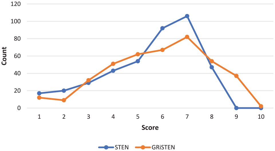
The number of respondents’ scores with STEN and GRiSTEN norms are demonstrated in Figures 7 to 10; STEN yields non-normal distribution of scores as if it were normal while GRiSTEN processes a non-normal distribution as it is. Thus, the scores provided by STEN and GRiSTEN differ. The horizontal axis in figures shows the STEN and GRiSTEN scores and the vertical axis shows the number of respondents with those scores.

Figure 7.

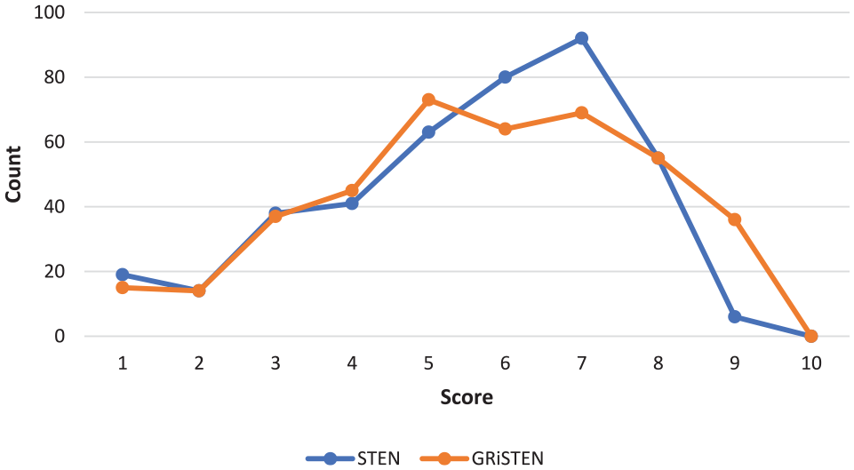
Comparative low velocity watch test for STEN and GRiSTEN scores.

Figure 8.

Comparative medium velocity watch test for STEN and GRiSTEN scores.

Figure 9.

Comparative high velocity watch test for STEN and GRiSTEN scores.

Figure 10.

Comparative watch performance score for STEN and GRiSTEN scores.

Low velocity watch test (Figure 7), medium velocity watch test (Figure 8), and high velocity watch test (Figure 9) graphics are made by transforming the total time lags presented by the respondent into norm scores.

Discussion

As it is clearly visible in this study, the distributions of each score are highly skewed. The skewness is a very common statistical fact that is usually overlooked (Newell & Hancock, 1984; Tsiang, 1972). As there is skewness, the arithmetic mean is formed away from the median, and it also generates a huge standard deviation (Ryu, 2011), which generates norms with STEN scores misleadingly (Fastenau et al., 1998). For all scores, the respondent must score a negative time lag in order to get 10 in STEN norm, which is definitely impossible.

When skewness is excessive, statisticians usually perform some arithmetic operations such as removing outliers, trimming the data, Box-Cox transformation (Sakia, 1992), and most frequently logarithmic transformation (Smith, 1993) in order to form a symmetry (Canay et al., 2017) and make both the arithmetic mean and standard deviation useful. Hence, not only is the data ruined at this stage but also “normal” outcomes are generated from “non-normal” data (Stevens, 1946).

It aims to obtain different “mean” and “deviation” outcomes from the scores with a method that takes skewness into account. For all scores, STEN is incapable of providing the most capable score, that is, 10. It cannot even provide 9 for medium velocity watch test and high velocity watch test. STEN norms tend to generate more “normal” norm-referenced scores (from 3 to 8) and less “extreme” norm-referenced scores (1, 2, 9, or 10). Having “dislocated” arithmetic mean and “huge” standard deviation caused by skewness reveal misleading norms with STEN method, but GRiSTEN generates fair norms. A norm-referenced scoring procedure which eventually becomes insufficient leads to ambiguity in the test results because it ends up with excessive normals or no extremes. Referring to GRiSTEN instead of STEN provides the correspondents with the ability to choose their “most capable” or “least capable” respondents regarding the test. Because GRISTEN produces outputs without distorting the nature of the distribution in spite of the existing deviance, it takes the contribution of each element in the data stack to the central point as the basis as a solution for the misleading effect of the deviance. Also, it produces two different parameters for the right and left tails. This capability of GRISTEN gives us the possibility of observing the real distribution, which is usually seen in nature and discriminates the extreme values (1, 2 and 9, 10). As an alternative to some of the drawbacks of STEN, the above mentioned superiorities of GRISTEN yields results which are much closer to the reality in the distorted data sets. Thus, a test user will be able to discriminate the differences among the individuals taking part in the test more clearly, and to make more effective interpretations.

In this study, we were able to generate more realistic norm scores on skewed data. Psychometrics is not the only area where norm scores are used. For example, in educational achievement and intelligence and attitude tests etc. norm-based scores are used. GRISTEN is open to use in different disciplines. New studies are needed on this subject.

Footnotes

Acknowledgements

Thanks to Mustafa Senocak, Bilisim Danismanlik, Ayhan Akcan, Hazal Aktas, and Sevgi Kilic for their contributions and support.

Data Availability Statement

The data used in this pilot study is available online. The research data and the computer codes used for calculation are hosted in the following public repository ().

Declaration of Conflicting Interests

The author declared no potential conflicts of interest with respect to the research, authorship, and/or publication of this article.

Funding

The author received no financial support for the research, authorship, and/or publication of this article.

ORCID iD

Mehmet Guven Gunver

References

Alfa-Electronics. (2018). Modern equipment for psychological and medical examinations of drivers. http://www.alfa-electronics.eu

Bornmann

(2013). The problem of percentile rank scores used with small reference sets. Journal of the American Society for Information Science and Technology, 64(3), 650. https://doi.org/10.1002/asi.22720

Brown

F. G.

(1976). Principles of educational and psychological testing. Holt, Rinehart and Winston.

Canay

I. A.

Romano

J. P.

Shaikh

A. M.

(2017). Randomization tests under an approximate symmetry assumption. Econometrica, 85(3), 1013–1030. https://doi.org/10.3982/ecta13081

Canfield

(1951). The “sten” scale-A modified C-scale. Educational and Psychological Measurement, 11(2), 295–297. https://doi.org/10.1177/001316445101100213

Clark-Carter

(2005). Stanine scores. In Everitt

B. S.

Howell

(Eds.), Encyclopedia of statistics in behavioral science (pp. 708–712). John Wiley. Ltd. https://doi.org/10.1002/0470013192.bsa640

Coaley

(2010). An introduction to psychological assessment and psychometrics. SAGE. https://doi.org/10.4135/9781446221556

Crocker

L. M.

Algina

(1986). Introduction to classical and modern test theory. Holt, Rinehart, and Winston.

Doane

D. P.

Seward

L. E.

(2011). Measuring skewness: A forgotten statistic? Journal of Statistics Education, 19(2), 1–18. https://doi.org/10.1080/10691898.2011.11889611

10.

Fastenau

P. S.

Denburg

N. L.

Mauer

B. A.

(1998). Parallel short forms for the boston naming test: Psychometric properties and norms for older adults. Journal of Clinical and Experimental Neuropsychology, 20(6), 828–834. https://doi.org/10.1076/jcen.20.6.828.1105

11.

Goldenratioinstatistics.com. (2020). Calculate. Author. http://goldenratioinstatistics.com/calculate.aspx

12.

GRiS Matlab. (2018). Researchgate. Author. https://www.researchgate.net/publication/326541004_GRiS_Matlab

13.

Gunver

M. G.

Senocak

M. S.

Vehid

(2018). To determine skewness, mean and deviation with a new approach on continuous data. Ponte International Scientific Researchs Journal, 73(2), 64–79. https://doi.org/10.21506/j.ponte.2018.2.5

14.

Gunver

M. G.

Senocak

M. S.

Yurtseven

(2017). Percentile based histogram bin width. Ponte International Scientific Researchs Journal, 73(3), 93–97. https://doi.org/10.21506/j.ponte.2017.3.10

15.

Mevasis | HPC Çözüm Ortağı. (2015, December 14). Time is your Value! Author. https://www.mevasis.com/

16.

Newell

K. M.

Hancock

P. A.

(1984). Forgotten moments. Journal of Motor Behavior, 16(3), 320–335. https://doi.org/10.1080/00222895.1984.10735324

17.

Pearson

(1920). The fundamental problem of practical statistics. Biometrika, 13(1), 1–16. https://doi.org/10.1093/biomet/13.1.1

18.

Pleace

(2016). Exclusion by definition: The under-representation of women in European homelessness statistics. In Mayock

Bretherton

(Eds.), Women’s homelessness in Europe (pp. 105–126). Palgrave Macmillan.

19.

Reznick

S. J.

(1989). Perspectives on behavioral inhibition (The John D. and Catherine T. MacArthur Foundation Series on Mental Health and Development) (1st ed.). University of Chicago Press.

20.

Rodriguez

(1997, January 23–25). Norming and norm-referenced test scores [Paper presentation]. Annual Meeting of the Southwest Educational Research Association, Austin, TX, United States. https://eric.ed.gov/?id=ED406445

21.

Ryu

(2011). Effects of skewness and kurtosis on normal-theory based maximum likelihood test statistic in multilevel structural equation modeling. Behavior Research Methods, 43(4), 1066–1074. https://doi.org/10.3758/s13428-011-0115-7

22.

Sakia

R. M.

(1992). The box-cox transformation technique: A review. The Statistician, 41(2), 169. https://doi.org/10.2307/2348250

23.

Shea

C. M.

Jacobs

S. R.

Esserman

D. A.

Bruce

Weiner

B. J.

(2014). Organizational readiness for implementing change: A psychometric assessment of a new measure. Implementation Science, 9(1). https://doi.org/10.1186/1748-5908-9-7

24.

Smith

R. J.

(1993). Logarithmic transformation bias in allometry. American Journal of Physical Anthropology, 90(2), 215–228. https://doi.org/10.1002/ajpa.1330900208

25.

Stevens

S. S.

(1946). On the theory of scales of measurement. Science, 103(2684), 677–680. https://doi.org/10.1126/science.103.2684.677

26.

Thompson

(1993). GRE percentile ranks cannot be added or averaged: A position paper exploring the scaling characteristics of percentile ranks, and the ethical and legal culpabilities created by adding percentile ranks in making “high-stakes” admission decisions. https://eric.ed.gov/?id=ED363637

27.

Tsiang

(1972). The rationale of the mean-standard deviation analysis, skewness preference, and the demand for money. The American Economic Review, 62, 221–248.

28.

Tummaruk

Kesdangsakonwut

Kunavongkrit

(2009). Relationships among specific reasons for culling, reproductive data, and gross morphology of the genital tracts in gilts culled due to reproductive failure in Thailand. Theriogenology, 71(2), 369–375. https://doi.org/10.1016/j.theriogenology.2008.08.003

29.

Whitaker

Wood

(2008). The distribution of scaled scores and possible floor effects on the WISC-III and WAIS-III. Journal of Applied Research in Intellectual Disabilities, 21(2), 136–141. https://doi.org/10.1111/j.468-3148.2007.00378.x