Healthcare Solutions for Children Who Stutter Through the Structural Equation Modeling and Predictive Modeling by Utilizing Historical Data of Stuttering

Abstract

Earlier studies established the role of demographic and temperamental features (DTFs) in the adaptation of childhood stuttering. However, these studies have been short on examining the latent interrelationships among DTFs and not utilizing them in predicting this disorder. This research article endeavors to examine latent interrelationships among DTFs in relation to childhood-stuttering. The purpose of the present is also to analyze whether DTFs can be utilized in predicting the likely risk of this speech disorder. Historical data on childhood stuttering was utilized for performing the invloved experiments of this research. “Structural-Equation-Modeling” (SEM) was applied to examine latent interrelationships among DTFs in relation to stuttering. The predictive analytics approach was employed to ensure whether DTFs of children can be utilized for predicting the likely risk of childhood-stuttering. SEM-based path analysis explored potential latent interrelationships among DTFs by separating them into categories of background and intermediate. By utilizing the same set of the DTFs, predictive models were able to classify children into stuttering and non-stuttering groups with optimal prediction accuracy. The outcomes of this study showed how the stuttering related historical data can be utilized in offering healthcare solutions for individuals with stuttering disorder. The outcomes of the present study also suggest that historical data on stuttering is a very rich source of hidden trends and patterns concerning this disorder. These hidden trends and patterns can be captured by applying a different type of structural and predictive modeling to understand the cause-and-effect relationship among variables in relation to stuttering. The SEM utilizes the cause-and-effect relationship among variables to explore latent-interrelationships between them. While predictive modeling utilizes the cause-and-effect relationship among variables to predict the possible risk of stuttering with optimal prediction accuracy.

Introduction

Historical data related to stuttering are valuable assets, comprising of concealed patterns and cause-and-effect relationships between variables representing risk factors and predictors. If such data is utilized for exploring interrelation among risk factors in relation to stuttering, then it is beneficial to understand the direct and indirect effect of risk factors over stuttering. This data can also be utilized to predict the likely risk of childhood stuttering. The outcomes of this approach will assist in the delivery of prior therapy and counseling for children. Therefore, this study sought to implement such computational methods that will expertise us to uncover these significant trends and hidden relationships among variables from historical data to predict future events. The predictive analytics approach is perfectly capable of examining causal-and-effect relationships from historical data of stuttering and bringing predictive capability into the outcomes to predict the likely risk of this speech disorder for unseen children’s population. This approach is extensively exercised to predict a variety of tasks from the range of elderly fall detection to the prediction of diseases and disorders (Bishop, 2006; Waheed & Sheik Abdul Khader, 2017).

Background of Childhood Stuttering

Most children are born healthy. Some exhibit certain developmental disorders such as attention-deficit, autism, hearing loss, intellectual disability, cognitive difficulties learning disorders, and speech disorders like childhood stuttering. In childhood stuttering, children face difficulties in forming words and sentences evenly. This speech disorder acts as a barrier for CWS in the development of their socio-academic life. Explicitly, children adopt childhood stuttering after the age of two. As they grow further and try to communicate, they normally start stuttering. There are a variety of factors like demographics, temperaments, genetics, and deformities in speech motor control that lead children to adapt to childhood stuttering. Of the factors, demographic (e.g., age, gender, and race) and temperamental features of children were indentified to be stimulating elements for the beginning of stuttering in children (Jones et al., 2014; Yairi & Ambrose, 2005).

Interconnection Between the DTFs and Childhood Stuttering

The outcomes of previous research studies revealed that demographic features affect children’s language development. Among demographics, gender and age are governing factors in persistence and recovery from childhood stuttering. For example, compared to females, males are more prone to stuttering. Likewise, the probability of childhood stuttering escalates up to 85% by age of three and a half years, but once they cross 4 years, they face a low associated threat of childhood stuttering (Yairi & Ambrose, 2005). Along with demographic features like age and gender, the Race of children has been included in the analysis to explore its role in relation to childhood stuttering.

On the other hand, children’s temperament also affects their language proliferation. (Rieser-Danner, 2003) specifically indicated that temperament may significantly impact an individual’s language development directly or indirectly. Furthermore, Jones et al. (2014) reported that temperament may be a causal factor in childhood stuttering. A considerable number of scientific investigations that have been carried out on CWS and fluent children to evaluate their temperamental variations are available (Anderson et al., 2003; Eggers et al., 2010; Kefalianos et al., 2017; Lewis & Golberg, 1997; Rocha et al., 2019). These scientific studies reported that many variations have been found between temperaments of CWS and children who not stutter (CWNS).

A bulk of temperaments such as self-control, intensity, effortful-control, discomfortness, approach, mood, aggressiveness, and adopting capabilities are found in children. Temperaments are defined as physiologically centered and atmosphere-inspired distinctions exhibited amongst people that influence their routine life activities and reactions (Goldsmith et al., 1987; Rothbart & Derryberry, 1981). Over time, these features become resilient and stay with them in all circumstances of their lives (Sanson et al., 2004). Not every child is born with the same set of temperaments. The variability in temperaments makes each child distinct and unique. Therefore, temperamental variations are reflected in their behavioral acclimation and language proliferation.

A majority of researchers and clinicians reported that temperament isn’t a singular attribute rather a group of related attributes (Goldsmith et al., 1987). Moreover, they intermingle with one another (Thompson et al., 1999). Therefore, it is essential to analyze how temperaments are grouped and interlinked with one another. As mentioned earlier, this study considered the demographics (e.g., age, gender, and race) of children along with their temperamental features to carry out experiments. These features were combined and referred to as the DTFs. The latent interrelationships among these features can be explored if they are separated into two categories such as background and intermediate. Latent interrelations among them would reveal their direct and indirect effect on persistence and recovery from childhood stuttering. On the other hand, the same features were utilized to check how much extent the potential risk its probable threat can be forecasted.

Contribution of the Present Study

• This study attempted to provide healthcare solutions concerning childhood stuttering by proposing the state of the art computational techniques in the form of “Structural Equation Modeling” (SEM) and “Predictive Analytics” through machine learning (ML).

• This study endeavors to examine the latent interrelationships of demographic and temperamental predictors and finding their role in predicting childhood stuttering.

• The outcomes of the present study would be robust and widely applicable since the underlined dataset called the DSP dataset is robust and scientific which is created by the prominent Scientist and Professor Tedra A. Walden and her team and is managed by Vanderbilt University.

• The outcomes that are generated by the SEM would make us understand latent interrelationships among demographic and temperamental predictors concerning childhood stuttering. On the other side, the predictive analytics approach of ML can bring predictive capability in the outcomes.

• The present study proved that the historical data on childhood stuttering is a very rich source of hidden trends and patterns in relation to stuttering. Hidden trends and patterns can be identified by building different types of structural and predictive models.

• The outcomes of this study would be a handful to several associates of this domain such as psychiatrists, SLPs, consultants, and research scholars.

Related Work

In this section, notable research studies have been presented that analyzed demographical and temperamental differences between CWS and CWNS in relation to childhood stuttering. In previous studies, among demographic factors, gender and age are found to be dominant factors in the persistence and recovery from stuttering. Compared to females, males are more prone to stutter. Children adopt childhood stuttering before the age of three. The probability of childhood stuttering escalated to 85% by the age of three and half years, but once they cross the age of four, they face a low associated threat of childhood stuttering (Yairi & Ambrose, 2005). Another empirical research was carried out on a hundred children (Rocha et al., 2019). They applied parametric tests to compare mean scores for the temperament, executive functioning, and anxiety of CWS and CWNS. In this study, it was seen that CWS exhibited significantly higher averages on the subscales of “anger/frustration, impulsivity, and sadness,” and lower scores on the “attention/focusing, perceptual sensitivity, and soothability/falling reactivity.” One more research study was performed on 39 children (Zengin-Bolatkale et al., 2018). They used the neutral, pleasant, and unpleasant stimulus to assess emotional reactivity and emotion regulation of CWS and CWNS. The “Analysis of Variance” (ANOVA) was applied to test their hypotheses. In this analysis, CWS were found to be more reactive to unpleasant stimuli than CWNS. Moreover, for CWS, they found that their temperament is linked with “cortical activity of emotion.” Kefalianos et al. (2017) have examined characteristics of 173 CWS of 3, 4, and 6 years. Temperament was observed to be a leading factor for stuttering severity while drawing a relationship between temperament and stuttering severity. In this study, it was also found that CWS who exhibited speech-blocks had a more complex temperament. Eggers et al. (2010) carried out a scientific study by taking a sample of 116 children (including both CWS and CWNS) for determining the association between this disorder and their temperamental trends. Temperamental data was collected via CBQ (“Children’s Behavior Questionnaire”). The ANOVA was utilized for data analysis to discover the substantive variation in amalgamated temperament factors between CWS and TDC (“Typically Developing Children”). This study reported a distinctive difference was found between CWS and TDC in their “inhibitory Control,” “attentional shifting,” “anger/frustration,” “approach,” and “motor activation.” Anderson et al. (2003) examined temperamental variations among 62 children via the “Behavioral Style Questionnaire” (BSQ). They employed statistical methods like “Multivariate analysis of variance” (MANOVA) for the analysis of temperamental data. It was concluded that CWS and CWNS were distinct in the temperamental features like “hyper-vigilance,” “non-adaptability to change,” and “irregular biological functions.” Choi et al. (2018) analyzed temperamental features reports of nearly 75 samples of both CWS and CWNS to uncover the influence of parents’ temperamental features on the CWS. The “Poisson distribution” and “Generalized Estimating Equations” were adopted to examine the data. The outcomes of this research suggest that stuttering is associated with certain psychological aspects of parents like positive and negative emotional reactivity. For analyzing affiliation between this disorder and emotional regulation and reactivity, a scientific study was conducted on 121 participants (including both CWS and CWNS) by Karrass et al. (2006). The temperamental data in this aspect were evaluated using MANOVA. The results of this investigation reveal that CWS were found to be considerably higher in emotion-reactivity, less in regulating emotions, and worse in attention regulation. Howell et al. (2004) investigated the association between fluency growth and temperament amongst CWS and CWNS by assessing temperaments via BSQ. Data were examined through “Fisher-Exact tests” and “independent t-tests.” This work suggests that CWS and CWNS could be discriminated against based on their temperaments irrespective of their language proficiency. Similarly, a scientific study was conducted by Felsenfeld et al. (2010) on a database of Dutch Twin Children comprising over 20,000 data records. Subjects were categorized into three classes: “Highly NonFluent,” “Typically Fluent,” and “Probable Stuttering” to assess their temperamental variations. The t-test and SPPS MIXED models were employed to examine the temperamental of these groups. This study reported that poor speech-fluency was an effect of a wider network of defective self-regulatory functions. Another study has been conducted to explore the link between stuttering and sleep problems (Jacobs et al., 2021). Authors reported evidence in the relation to stuttering and sleep issues by indicating that individuals who are suffering from this speech disorder sleep 20 minutes less than normal peers. Authors also highlighted that stutterers were twice as likely as those who did not stammer to have difficulty sleeping or staying asleep (15%). A study was conducted to analyze the temperaments of children who stutter and not stutter (Rodgers & Jackson, 2021). It was asserted that stutterers’ temperament may be thought of as a mirror through which they react to anticipation. Some of studies used machine learning algorithms like Artificial Neural Networks (ANN), K-Nearest Neighbors (KNN), and Support Vector Machine (SVM) were used to classify fluent and dysfluent speech (Kushwaha & Kumar, 2017; Wisniewski & Kuniszyk-Jojkowiak, 2015). Few of researchers analyzed the neuro-anatomical differences using MRI data of children and adults who stutter (Zengin-Bolatkale et al., 2018).

As we know, emotions are integral parts of temperaments that can be quantified and analyzed to explore their complexity level. Because of this, a novel EEG-based approach was presented for processing emotions of a particular category of participants (Waheed et al., 2021). In line with the previous research, an EEG-based sensor was utilized to assess emotional regulation among the adult population who suffer from this disorder (Waheed & Abdul Khader, 2020). It was reported that stuttering adults were found to be weak in emotion regulation against visual stimuli. This research approach can further be extended to the children population who stutter for the same purpose.

Objectives of this Study

In the aforementioned research studies, we found two major limitations. The first limitation was that prior research studies had efficiently attempted to identify demographical and temperamental differences between CWS and CWNS in relation to childhood stuttering. However, no attempts had been made to explore latent interrelationships among the DTFs concerning childhood stuttering. Exploring the latent interrelationships among the DTFs could prove to be beneficial to understand their direct and indirect effect on childhood stuttering. Their latent interrelationships could be explored if we attempt to separate them into two groups as the background and the intermediate. To explore interrelationships among the DTFs, this study attempts to propose a conceptual model. The second limitation was that most of the previous research studies did not apply any automated computation approaches to bring predictive capability in the results of stuttering researches. They mainly focused on “within-group analysis of CWS groups” and “comparing the mean difference of temperamental traits amongst CWS and CWNS.” It shows that earlier research works have been observational and lacked prediction capability for the untested population of children. Similar limitations have also been reported in the above-mentioned studies. For obtaining enhanced and more accurate results on childhood stuttering, adopting a machine learning approach was recommended (Jones et al., 2014). Therefore, to bring predictive capability in the results of stuttering, this study proposes a machine-learning-based predictive analytics approach. The present study defines two main objectives. The first objective is to explore potential interrelationships among the DTFs in relation to childhood stuttering. The second objective is to affirm whether predicting the probable risk of childhood stuttering is achievable utilizing historical data records about DTFs of children. A couple of hypotheses were set. First, it was assumed that the implemented conceptual model will have a good fit with utilized historical data of the DTFs. Second, children’s DTFs can have a significant contribution in the process of prediction of the probable threat of this disorder.

Method

The proposed methodology to carry out the current investigation has been depicted in Figure 1.

Figure 1.

Flowchart representing the proposed methodology to carry out the current study.

The Dataset Selection

Both SEM and predictive analytics need relevant research-oriented historical data to construct analytical models. Structural models use stuttering historical data to explore interrelationships among data variables in relation to the dependent variable representing childhood stuttering. On the other side, predictive models capture latent trends and patterns and cause-and-effect bindings among variables. Historical data should include data observations about both positive and negative cases to capture latent interrelationships and cause-and-effect relationships. Accordingly, to fetch the required data records about the DTFs, an open-access dataset, named, “Developmental Stuttering Project” (DSP) was chosen. It consists of DTFs based historical data records of the CWS as experimental group and CWNS as the control group. However, its creators have not reported any information regarding how many CWS have recovered from stuttering during the period of research. The download links of this dataset were given after references in the supplement section of this article. In Table 1, the summary of the DSP dataset has been presented.

Table 1.

Summary of DSP Dataset.

The aim of elect, the dataset: To utilized available data records on the DFTs of CWS and CWNS for accomplishing objectives and testing hypotheses.

Constitutes: Research-based historical data records on the DTFs of CWS and CWNS. Designed by: Professor Tedra Walden and her colleagues. Maintained by: Vanderbilt University, USA.

Demographic details of subjects: Experimental group: This group involves subjects belongs to CWS. Control group: This group consists of subjects belongs to CWNS. Age range: 3–7 years, Avg. Age: 4 years Subjects races: White, American Indian or Alaska Native, Asian or African American, and Hawaiian.

No. of variables available related to the DTFs: 35

Applied criteria to categorize subjects into CWS and CWNS: The creators of the dataset applied below estimations to categorized subjects, (a) If children’s total of Stuttering Siverity Instrument (SSI_total) ≥11, then such children were labeled as CWS, (b) If children’s SSI_total <11, then such children were labeled as CWNS

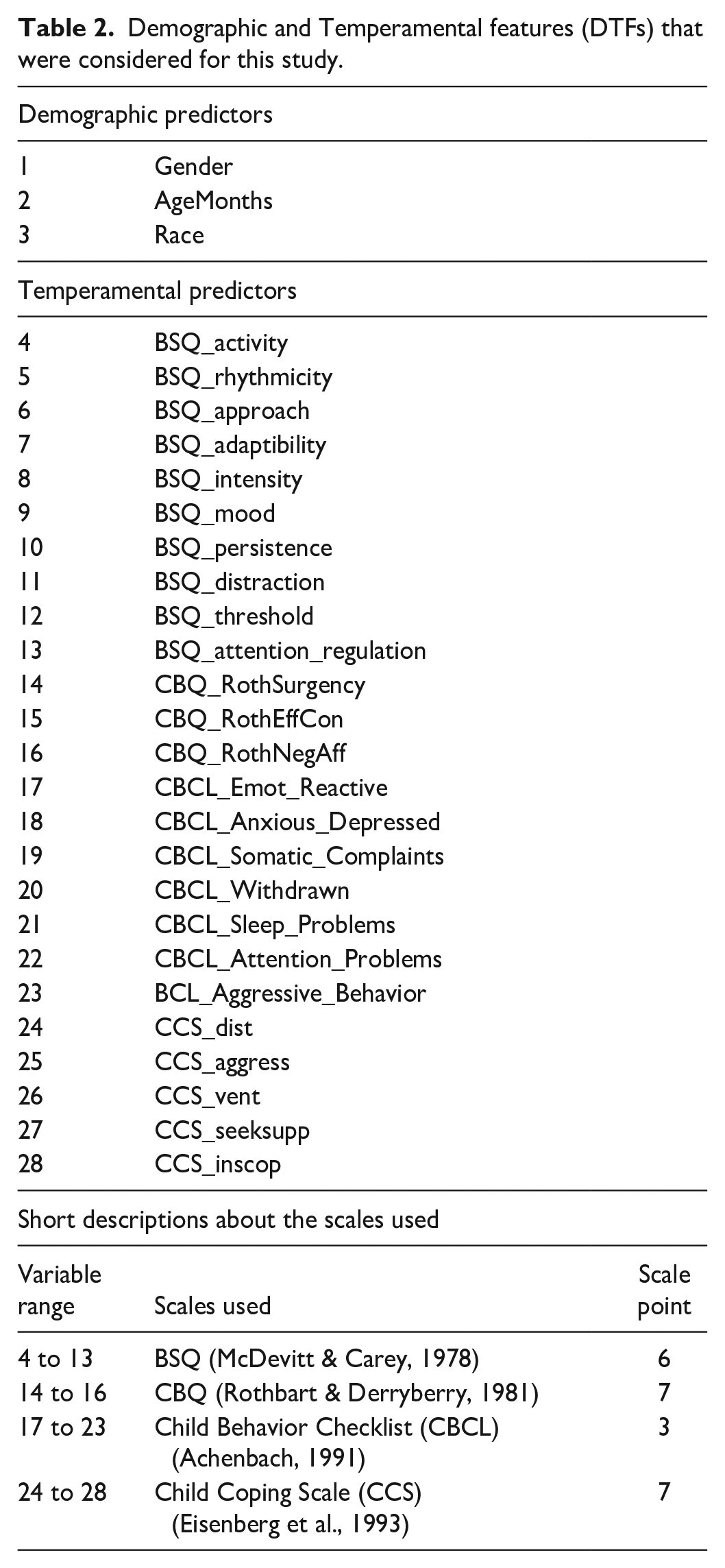
This dataset constitutes a large chunk of 35 variables representing the DTFs. In this chunk, some of the variables were identified to be highly correlated. Hence, such variables were discarded correlating cut-off values of 70% and above because such variables affected the prediction accuracy. Finally, the leftover 28 variables were utilized for the rest of the experiments as independent variables (see Table 2).

Table 2.

Demographic and Temperamental features (DTFs) that were considered for this study.

Demographic predictors
1	Gender
2	AgeMonths
3	Race
Temperamental predictors
4	BSQ_activity
5	BSQ_rhythmicity
6	BSQ_approach
7	BSQ_adaptibility
8	BSQ_intensity
9	BSQ_mood
10	BSQ_persistence
11	BSQ_distraction
12	BSQ_threshold
13	BSQ_attention_regulation
14	CBQ_RothSurgency
15	CBQ_RothEffCon
16	CBQ_RothNegAff
17	CBCL_Emot_Reactive
18	CBCL_Anxious_Depressed
19	CBCL_Somatic_Complaints
20	CBCL_Withdrawn
21	CBCL_Sleep_Problems
22	CBCL_Attention_Problems
23	BCL_Aggressive_Behavior
24	CCS_dist
25	CCS_aggress
26	CCS_vent
27	CCS_seeksupp
28	CCS_inscop
Short descriptions about the scales used
Variable range	Scales used	Scale point
4 to 13	BSQ (McDevitt & Carey, 1978)	6
14 to 16	CBQ (Rothbart & Derryberry, 1981)	7
17 to 23	Child Behavior Checklist (CBCL) (Achenbach, 1991)	3
24 to 28	Child Coping Scale (CCS) (Eisenberg et al., 1993)	7

This study applied two state-of-the-art methods to achieve its objectives. The first method is the SEM. While the second method is Predictive Analytics. The below paragraphs provide details about the implementation of the aforementioned methods.

Implementing the Proposed Conceptual Model to Investigate the Interrelationships Among the DTFs Concerning Childhood Stuttering

The majority of researchers and clinicians reported that temperament is not a singular attribute, but a group of related attributes (Goldsmith et al., 1987). Moreover, temperaments inter-mingle with one another (Thompson et al., 1999). Therefore, it is essential to analyze how temperaments are grouped and interlinked with one another. As explained earlier, in this study, the demographic features (e.g., age, gender, and race) were added along with the temperamental features (and termed them as DTFs) of children to evaluate their combined latent interrelationships in relation to childhood stuttering. The latent interrelationships among the DTFs with stuttering could be explored if they are separated into two categories such as the background and the intermediate as shown in Figure 2. In addition, explored interrelationships among the DTFs would also reveal their positive and negative impact on childhood stuttering.

Figure 2.

Proposed conceptual model illustrating potential interconnections between the DTFs as background and intermediate variables in relation to persistence and recovery from childhood stuttering.

Thus, to develop the proposed conceptual model presented in Figure 2, we found the SEM to be the most efficient statistical tool. SEM-based analysis facilitates establishing interrelations among independent variables by separating them into two categories like the background and the intermediate (Kline, 2016; Schumacker & Lomax, 2004). The involved experiments of this analysis were performed on IBM’s Amos software. To the SEM-based analysis, a set of DTFs that is tabulated in Table 2 were provided as predictors against the dependent variable, named, “SSI_total.” The response variable is a numeric representing children’s score in relation to childhood stuttering. In the DSP dataset, this variable is described as children’s scoring regarding Stuttering Severity Instrument (SSI). The SSI is the total of frequency_of_stuttering, duration_of_stuttering, and physical_concomitants.

Amos’s Integrated Development Environment (IDE) provides working space to develop SEM-based modeling as depicted in Figure 3. The SEM performs two key operations during model building such as the “path-analysis” and the “multivariate regression analysis” to analyze the latent association among variables in relation to an outcome variable (Kline, 2016; Schumacker & Lomax, 2004). Commonly, the SEM-based model building involves two types of variables, namely, the observed variables and the latent variables. However, in this model building, only the observed variables were needed, and the latent variables were not required. Essentially, the observed variables are manifest variables that are denoted by a rectangle symbol. The observed variables can act as both exogenous and endogenous variables. The exogenous variables are generally used to represent background variables. These variables are similar to independent variables for which empirical data (like the DSP dataset) are required in the study. On the other hand, endogenous variables can play the role of both intermediate variables and the outcome variable of the model (see Figure 5).

Figure 3.

Illustrates the graphical user interface of IBM’s Amos software that was utilized to implement the conceptual model presented in Figure 2.

In the present analysis, the path-analysis on the DTFs was performed using the “Exploratory Factor Analysis” (EFA) approach of SEM. In the EFA, the path-analysis is performed for examining the latent interrelationships among observed variables without imposing a preconceived structure on the outcome variable. Hence, the path-analysis was extensively performed based on the trial-and-error method to fit the model over the independent variables to find their relationship with the dependent variable.

Determining the Role of DTFs in Predicting the Potential Risk of Childhood Stuttering Through Predictive Analytics Approach

In this subsection, the approch of predictive analytics was employed to create predictive models to determine the role of DTFs in predicting the potential risk of childhood stuttering. R studio was used to perform the involved experiments. To implement predictive analytics, the set of variables presenting DTFs from Table 2 were provided as independent variables against the dependent variable, named, “talkergroup_SSI.” As per its description provided in the DSP dataset, this dependent variable is categorical has two predictive labels, named, CWS and CWNS. The labels of this dependent variable were created based on the SSI score of talker groups. Here, the talker groups represent participants of two types like CWS and CWNS. The children who scored SSI_total ≥11, were labeled as CWS. While, children who scored SSI_total <11, such children were labeled as CWNS.

As mentioned earlier, the DSP dataset consists of historical data records on the DTFs of the experimental group (i.e., CWS) and the control group (i.e., CWNS). Hence, this study seeks to take advantage of this dataset for predicting the likely threat of childhood stuttering using the predictive analytical approach based on children’s historical data records about the DTFs. Its working philosophy has been depicted in Figure 4a. In this approach, the predictive models are created to capture the latent cause-and-effect relationships among the data variables present in the provided training data. Later, these models are utilized for predicting future events when the unseen data is provided. In this study, along with prominent ML algorithms such as SVM, the other two algorithms like RF and kNN have been applied for building the predictive models.

Figure 4.

(a) Illustrates the working philosophy of the predictive analytics for the prediction of the likely threat of stuttering in children. The DTFs were considered as predictors against the dependent variable. (b) Depicts the working philosophy of ML’s training-testing paradigm that was applied during the development of predictive models.

The SVM is a well-suited classifier for small, non-linear, and complex datasets like the “DSP dataset” having a large number of features. Further, it is deterministic, and therefore, avoids over-fitting of predictive models. It uses “Radial Basis Function” as a kernel tricks to classify non-linear instances of data. Next, RF is one of the ensemble techniques that combine the sequence of m learned models to build improved classification models. RF adopts a majority voting approach to classify as CWS and CWNS. On the other hand, kNN is based on an approach like learning by analogy (Han et al., 2001).

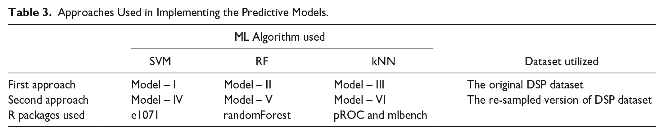
Predictive models have been implemented based on ML’s training-and-testing architecture. The working philosophy of this architecture in reference to these algorithms is depicted in Figure 4b. In this architecture, predictive models are trained over training data and then tested upon testing data. The training data acts as known-data for predictive models, while the testing-set plays the role of unknown-data for predictive models. The implementation of the predictive models has been performed using the two approaches as shown in Figure 1 and Table 3. In the first approach, three separate predictive models have been created by training and testing them over the original DSP dataset. Whereas, in the second approach, the DSP dataset’s re-sampled form was utilized to train and test the predictive models.

Table 3.

Approaches Used in Implementing the Predictive Models.

	ML Algorithm used			Dataset utilized
	SVM	RF	kNN
First approach	Model – I	Model – II	Model – III	The original DSP dataset
Second approach	Model – IV	Model – V	Model – VI	The re-sampled version of DSP dataset
R packages used	e1071	randomForest	pROC and mlbench

The First Approach

First of all, the dataset was partitioned into a training set (70%) and a testing set (30%). A dataset can be partitioned into training and testing set in several ratios like 50:50, 60:40, and 80:20. However, the present study partitioned the dataset with ratio of 70:30 to supply appropriate amount of data records to the training phase of the predictive models as the selected dataset is moderate in size. This ratio will prevent predictive models to get underfitted over the dataset. Then, the predictive models have been trained upon the training set with 10-fold cross-validation. In this cross-validation, the training set is randomly divided into 10-folds of equal size. Each time the model is trained on nine folds and tested on the 10th fold. The process is repeated 10 times. This approach effectively trains the models and avoids their over-fitting with the training data. Let us understand the working of the predictive models in the context of predicting childhood stuttering. First, during the training phase, these models capture the hidden cause-and-effect relationships present in the training data samples of the DTFs in relation to the outcome variable. After been trained, during the testing phase, the generalizability of their results is tested by providing unknown data samples of the DTFs in the form of the testing set. The predicted results of these models were shown in Section – A of Tables 6 and 7.

The Second Approach

Before predictive model building, the re-sampling of the original DSP dataset was carried out to make it well-balanced. Two kinds of imbalances were observed in the original dataset. The first imbalance was in the form of an inadequate ratio of data samples per predictor. The available ratio was 4:1; however, the recommended minimal ratio between them to implement a multivariate analysis is 10:1 (Hair et al., 2014). The second imbalance was in terms of the uneven distribution between the number of samples in the predictive classes that is, CWS and CWNS. As, we observed that the samples of the interested class that is, CWS were in minority (57), whereas the samples belonging to the CWNS are in majority (81). If the dataset is unevenly distributed between its predictive classes, the predicted results would be skewed towards the majority class. Therefore, the re-sampling of this dataset has been performed by applying the “Synthetic Minority Over-sampling Technique” (SMOTE). The SMOTE not only synthetically creates new data samples for the interested minority class, but also relatively increases the overall sample size of the dataset. To apply SMOTE as per the need of this study, we have modified the pseudo-code of original SMOTE proposed by Chawla et al. (2002), and it has been presented in Table 4.

Table 4.

Modified SMOTE Pseudocode for Re-sampling DSP Dataset.

Algorithm SMOTEforDSPdataset(M, S, k)
Input: M: no. of observations that is, samples that belong to the minority class that is, CWS (here, M = 57); S: percent of SMOTE (here, we set S = 300; k: no. of the nearest neighbors (here, we set k = 3)
Output: Synthetic observations for CWS := (S/100)*M
1:	S := (int) (S/100) [amount of SMOTE was assumed]
2:	k := no. of nearest neighbors
3:	numatt = no. of attributes
4:	Observations[][]: array of original CWS class
5:	countSynth: keeps records of the no. synthetic observations generated, initial value is 0
6:	synthObservations[][]: array of synthetic observations
7:	for j := 1 to M
8:	Calculate k nearest neighbors for j, and populate the indices in the mmarray
9:	Store(S, j, mmarray)
10:	End
11:	Function Store(S, j,mmarray) [this is the function to yield synthetic observations]
12:	while S ≠ 0
13:	Select any random no. between 1 and k, all it mm. It will choose one k nearest neighbors of j
14:	for att := 1 to numatt
15:	Calculate: diff := Observations[mmarray[mm]][att] – Observation [j][att]
16:	Calculate: distance := randomNumber between 0 and 1
17:	SynthObservations[countSynth][att] = Observation[j][att] + distance * diff
18:	End
19:	countSynth++
20:	S := S – 1
21:	End
22:	return [End of Function]
	End of PseudoCode

The Pseudocode presented in Table 4 depicts that this process identifies a feature-vector and its nearest neighbor, and it then takes a difference between the two. Later, it multiplies the difference with a random number between 0 and 1. Further, it identifies a new point on the line segment by adding a random number to the feature-vector. It repeats this process for the identified feature-vectors. As a result, we finally obtained a balanced number of data samples between CWS (171) and CWNS (171) through an increased number of samples up to 342.

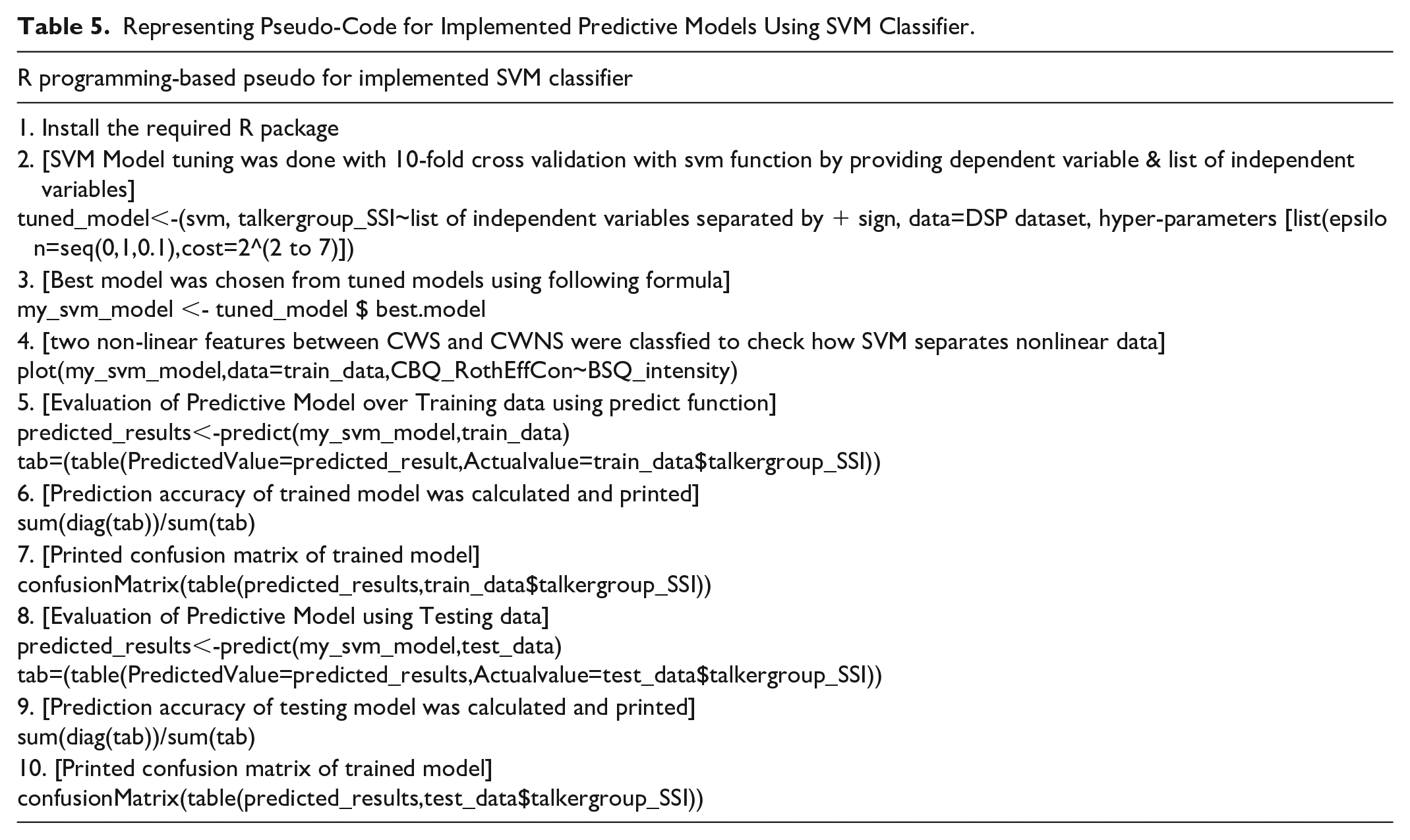
In the end, the re-sampled version of the DSP dataset was partitioned into a training set (70%) and a testing set (30%). Like predictive models developed in the first approach, the next three predictive models of this approach have been created by training and testing them against the training set and testing sets. The generalized pseudo-codes of implemented models using classifiers like the SVM, the RF, and the kNN are presented in Tables 5 to 7.

Table 5.

Representing Pseudo-Code for Implemented Predictive Models Using SVM Classifier.

R programming-based pseudo for implemented SVM classifier
1. Install the required R package
2. [SVM Model tuning was done with 10-fold cross validation with svm function by providing dependent variable & list of independent variables]tuned_model<-(svm, talkergroup_SSI~list of independent variables separated by + sign, data=DSP dataset, hyper-parameters [list(epsilon=seq(0,1,0.1),cost=2^(2 to 7)])
3. [Best model was chosen from tuned models using following formula]my_svm_model <- tuned_model $ best.model
4. [two non-linear features between CWS and CWNS were classfied to check how SVM separates nonlinear data]plot(my_svm_model,data=train_data,CBQ_RothEffCon~BSQ_intensity)
5. [Evaluation of Predictive Model over Training data using predict function]predicted_results<-predict(my_svm_model,train_data)tab=(table(PredictedValue=predicted_result,Actualvalue=train_data$talkergroup_SSI))
6. [Prediction accuracy of trained model was calculated and printed]sum(diag(tab))/sum(tab)
7. [Printed confusion matrix of trained model]confusionMatrix(table(predicted_results,train_data$talkergroup_SSI))
8. [Evaluation of Predictive Model using Testing data]predicted_results<-predict(my_svm_model,test_data)tab=(table(PredictedValue=predicted_results,Actualvalue=test_data$talkergroup_SSI))
9. [Prediction accuracy of testing model was calculated and printed]sum(diag(tab))/sum(tab)
10. [Printed confusion matrix of trained model]confusionMatrix(table(predicted_results,test_data$talkergroup_SSI))

Table 6.

Displaying Pseudo-Code for Implemented Predictive Models Using RF Classifier.

R programming-based pseudo for implemented RF classifier
1. Install required R package
2. [RF-based predictive model creation by providing dependent variables & list of independent variables using randomForest function]my_rf_model <- randomForest(talkergroup_SSI~list of independent variables seperated by + sign, data=train_data, hyperparametes [ntree=750, mtry = 5, importance = TRUE, proximity = TRUE])
3. [Evaluation of Predictive Model over Training data using predict function]Prediction_over_train_data <- predict(my_rf_model, train_data)
4. [Printing confusion matrix of trained model]confusionMatrix(Prediction_over_train_data, train_data$talkergroup_SSI)
5. [Evaluation of Predictive Model over Testing data using predict function]Prediction_over_testing_data <- predict(my_rf_model, test_data)
6. [Printing confusion matrix of tested model]confusionMatrix(Prediction_over_testing_data, test_data$talkergroup_SSI)
7. [Printing top 20 variables of Importance using varImpPlot function]varImpPlot(my_rf_model, sort = T, n.var = 20,main = “Top 20 - Variable Importance”)importance(my_rf_model)
8. [Model was tuned for mtry using tuneRF function upon train_data]tuned_model <- tuneRF(train_data[,-29], train_data[,29], stepFactor = 0.5, plot = TRUE, ntreeTry = 300, trace = TRUE, improve = 0.05)Here, variables like stepFactor, ntreeTry, improve are hyper parameters

Table 7.

Showing Pseudo-Code for Implemented Predictive Models Using kNN Classifier.

R programming-based pseudo for implemented kNN classifier
1. Install R package
2. [Computational naunces of kNN were set using trainControl method]tr_Control <- trainControl(method = “repeatedcv,” number = 10, repeats = 3, classProbs = TRUE,summaryFunction = twoClassSummary)Here, variables like number, repeats, ClassProbs, summaryFunction are hyperparameters
3. [Training kNN-based predictive model using train function by providing dependent variables & list of independent variables using randomForest function]my_kNN_model <- train(talkergroup_SSI ~ list of independent variables separated by + sign, data=train_data, method = “knn,” tuneLength = 20, trControl = tr_Control, preProc = c(“center,” “scale”),metric = “ROC”)Here, variables like tuneLenght, trControl, preProc, metric are hyper parameters
4. [Evaluation of Predictive Model over Testing data using predict method]predicted_cases <- predict(my_kNN_model, newdata = test_data)
5. [Printing confusion matrix of tested model]confusionMatrix(predicted_cases, test_data$talkergroup_SSI)
6. [Plotting top 20 variables of Importance using varImp method]varImp(my_kNN_model)

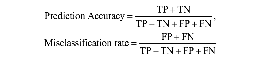
Evaluating the performance of predictive models

The performance of the predictive models is evaluated against major metrics such as prediction accuracy, percentage of sensitivity and specificity, precision, recall, and F-score (Han et al., 2001) The sensitivity refers to how correctly the positive cases were predicted by the model. In this study, the positive cases refer to the subjects having stuttering that is, CWS. While specificity refers to how correctly the negative cases that is, CWNS were predicted by the model. Further, the precision score indicates the relevancy in the prediction results whereas the recall score signifies how the model was able to capture truly relevant results. On the other hand, the F-score indicates the harmonic mean between the precision and the recall. Therefore, the higher scores of sensitivity, precision, recall, and the F-score indicates that a particular model is a good performer. These metrics are estimated using the formula (Han et al., 2001):

$$\begin{array}{l}\mathrm{Prediction}\mathrm{Accuracy}=\frac{\mathrm{TP}+\mathrm{TN}}{\mathrm{TP}+\mathrm{TN}+\mathrm{FP}+\mathrm{FN}},\\ \mathrm{Misclassification}\mathrm{rate}=\frac{\mathrm{FP}+\mathrm{FN}}{\mathrm{TP}+\mathrm{TN}+\mathrm{FP}+\mathrm{FN}}\end{array}$$

$$\mathrm{Specificity}=\frac{\mathrm{TN}}{\mathrm{TN}+\mathrm{FP}},\mathrm{Sensitivity}=\frac{\mathrm{TP}}{\mathrm{TP}+\mathrm{FN}}$$

$$\mathrm{Recall}=\frac{\mathrm{TP}}{\mathrm{TP}+\mathrm{FN}}$$

$$\mathrm{Precision}=\frac{\mathrm{TP}}{\mathrm{TP}+\mathrm{FP}},\mathrm{F}-\mathrm{score}=2\left(\frac{\mathrm{Precision}\mathrm{x}\mathrm{Recall}}{\mathrm{Precision}+\mathrm{Recall}}\right)$$

Results

Understanding Results Produced from the Implemented Conceptual Model

Figure 5 depicts the SEM-based conceptual model that has been resulted after an extensive path analysis. This model represents how the DTFs-based variables were separated into categories of intermediate and background. The model also depicts that the intermediate variables have been resulting in a hierarchy of first and second levels. From Figure 5, it is seen that the model was made of 29: the observed variables, 10: the unobserved variables, 28: the exogenous variables, and 9: the endogenous variables.

Figure 5.

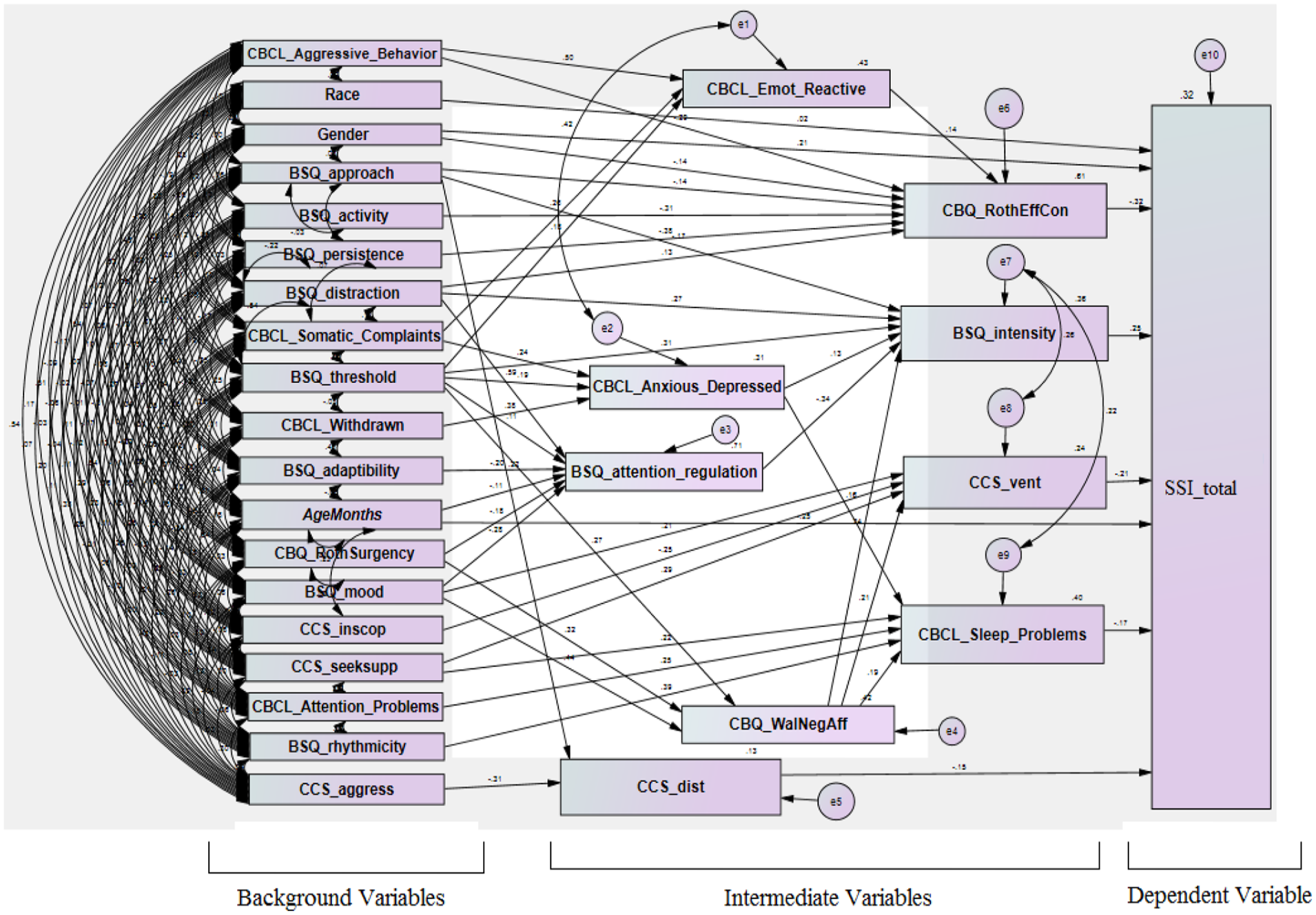
Resultant SEM-based conceptual model that depicts interrelations among the DTFs in relation to the dependent variable by separating them into the background and intermediate categories.

The SEM-based path-analysis traces paths to link intermediate variables with background ones. The path-analysis also entails the direct and indirect connections between the measured or the latent variables. Figure 5 depicts that among the DTFs, during the path analysis, features such as aggressive-behavior, gender, approach, distractions, somatic-complaints, threshold, age, surgency, mood, and seek-support were traced as background variables. Among traced background variables, many variables acted over two or more pathways to get connected with the intermediate variables. Some of them acted over a single path to get connected with the intermediate variables. On the other hand, among the DTFs, features like effortful-control, intensity, sleeping-problems, “coping by venting,” and “coping by distancing” were fallen into the category of intermediate variables. Figure 5 also shows that the feature threshold that was traced as a background variable, acted over eight different indirect paths to be linked with the dependent-variable, named, SSI_total. Its first indirect path to get connected with the dependent-variable was via emotional-reactivity and effortful-control. Its second indirect path was through variable intensity. Its third and fourth indirect paths involving variable anxious-depressed are via variables like intensity and sleep-problems respectively. Its fifth indirect path was via variables, named, attention-regulation and intensity. Finally, its sixth, seventh, and eighth indirect paths involving variable negative-affectivity via variables like sleep problems, vent, and intensity respectively.

Thus, the implemented conceptual model efficiently separated DTFs into categories of background and intermediate while exploring their significant relationship with childhood stuttering. Besides, the intermediate variables were sub-categorized into the first and second levels. For example, features such as emotional-reactive, anxious-depressed, attention-regulation, and negative-affectivity have emerged as the first-level intermediate variables. While, traits like effortful-control, sleep problems, intensity, and coping by venting and distancing resulted as the second-level intermediate variables. On the other hand, the features like Gender and AgeMonths exhibited a direct relation with childhood stuttering.

Table 8 present the model’s estimations of “multivariate regression” analysis.

Table 8.

Reporting of Parameter Estimations for the Model in Figure 5.

S. No.	Variables	B	S.E. of B	b	t-Value	p-Value
1	CBQ_WalNegAff <--- BSQ_mood	0.496	0.075	0.438	6.587	***
2	CBQ_WalNegAff <--- BSQ_threshold	0.323	0.080	0.269	4.052	***
3	CBCL_Emot_Reactive <--- CBCL_Aggressive_Behavior	0.171	0.021	0.504	8.165	***
4	CBCL_Emot_Reactive <--- BSQ_threshold	0.675	0.260	0.178	2.599	.009
5	CBCL_Emot_Reactive <--- CBCL_Somatic_Complaints	0.309	0.084	0.256	3.665	***
6	CBCL_Anxious_Depressed<--- CBCL_Somatic_Complaints	0.275	0.087	0.245	3.167	.002
7	CBCL_Anxious_Depressed <--- CBCL_Withdrawn	0.533	0.095	0.381	5.583	***
8	CBCL_Anxious_Depressed <--- BSQ_threshold	0.657	0.267	0.185	2.463	.014
9	BSQ_attention_regulation <--- CBQ_RothSurgency	−0.069	0.018	−0.179	−3.767	***
10	BSQ_attention_regulation <--- BSQ_distraction	0.406	0.039	0.591	10.475	***
11	BSQ_attention_regulation <--- BSQ_mood	−0.212	0.048	−0.282	−4.425	***
12	BSQ_attention_regulation <--- BSQ_adaptibility	−0.146	0.046	−0.198	−3.172	.002
13	BSQ_attention_regulation <--- AgeMonths	−0.005	0.002	−0.106	−2.289	.022
14	BSQ_attention_regulation <--- BSQ_threshold	0.091	0.046	0.114	1.969	.049
15	CBQ_WalNegAff <--- CBQ_RothSurgency	0.188	0.038	0.323	4.956	***
16	CBQ_RothEffCon <--- BSQ_persistence	−0.465	0.071	−0.380	−6.518	***
17	CBCL_Sleep_Problems <--- CCS_seeksupp	0.538	0.158	0.222	3.405	***
18	CBQ_RothEffCon <--- BSQ_activity	−0.380	0.074	−0.313	−5.130	***
19	CCS_vent <--- CCS_seeksupp	0.347	0.091	0.287	3.797	***
20	CBQ_RothEffCon <--- BSQ_distraction	0.131	0.059	0.126	2.216	.027
21	CBQ_RothEffCon <--- CBCL_Aggressive_Behavior	−0.031	0.008	−0.288	−4.021	***
22	CBQ_RothEffCon <--- BSQ_approach	−0.129	0.049	−0.142	−2.645	.008
23	CBCL_Sleep_Problems <--- BSQ_rhythmicity	1.584	0.270	0.388	5.875	***
24	CCS_vent <--- BSQ_mood	0.447	0.186	0.206	2.408	.016
25	CCS_vent <--- CBQ_WalNegAff	0.401	0.165	0.209	2.430	.015
26	CBCL_Sleep_Problems <--- CBCL_Attention_Problems	0.365	0.098	0.248	3.738	***
27	CCS_vent <--- CCS_inscop	−0.266	0.084	−0.245	−3.183	.001
28	CBQ_RothEffCon <--- Gender	−0.190	0.074	−0.140	−2.567	.010
29	CBCL_Sleep_Problems <--- CBCL_Anxious_Depressed	0.209	0.090	0.160	2.327	.020
30	CBQ_RothEffCon <--- CBCL_Emot_Reactive	0.045	0.021	0.141	2.161	.031
31	BSQ_intensity <--- BSQ_approach	−0.124	0.049	−0.174	−2.530	.011
32	BSQ_intensity <--- BSQ_threshold	0.290	0.082	0.306	3.522	***
33	BSQ_intensity <--- BSQ_attention_regulation	−0.402	0.115	−0.339	−3.503	***
34	BSQ_intensity <--- BSQ_distraction	0.218	0.081	0.268	2.710	.007
35	BSQ_intensity <--- CBCL_Anxious_Depressed	0.035	0.019	0.131	1.863	.062
36	BSQ_intensity <--- CBQ_WalNegAff	0.191	0.061	0.242	3.110	.002
37	CCS_dist <--- BSQ_approach	0.230	0.086	0.215	2.679	.007
38	CCS_dist <--- CCS_aggress	−0.180	0.047	−0.307	−3.816	***
39	CBCL_Sleep_Problems <--- CBQ_WalNegAff	0.743	0.264	0.192	2.816	.005
40	Dev_Stuttering <--- CCS_vent	−1.180	0.421	−0.210	−2.800	.005
41	Dev_Stuttering <--- BSQ_intensity	3.398	1.061	0.248	3.202	.001
42	Dev_Stuttering <--- CBQ_RothEffCon	−3.475	0.814	−0.323	−4.268	***
43	Dev_Stuttering <--- Race	0.152	0.447	0.024	0.339	.734
44	Dev_Stuttering <--- AgeMonths	−0.200	0.058	−0.247	−3.482	***
45	Dev_Stuttering <--- Gender	3.035	1.081	0.208	2.808	.005
46	Dev_Stuttering <--- CBCL_Sleep_Problems	−0.472	0.211	−0.169	−2.235	.025
47	Dev_Stuttering <--- CCS_dist	−1.393	0.643	−0.153	−2.165	.030

Note. B = unstandardized coefficient; SE = standard error; b = standardized coefficient.

Evaluating the Performance of the Implemented Conceptual Model Presented in Figure 5

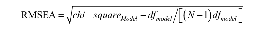
The consistency of the model with the utilized research data was validated upon the major statistical parameters like RMSEA, GFI, NFI, CFI, and TLI, and results were presented in Table 9 (Byrne, 2016; Kline, 2016).

Table 9.

Summary of Performance Metrics of the Model in Figure 5.

Types of model fit	Indices	Obtained value	Suggested value
Absolute fit	Chi-square value	235.918	–
	Df	185	–
	RMSEA	0.045	<0.08 (Hair et al., 2014)
	GFI	0.900	>0.90 (Hu & Bentler, 1999)
Incremental fit	AGFI	0.766	>0.90 (Hair et al., 2014)
	CFI	0.964	>0.90 (Hooper et al., 2008)
	NFI	0.869	>0.90 (Hu & Bentler, 1999)
	TLI	0.920	>0.90 (Schumacker & Lomax, 2004)
Parsimonious fit	Chi_square/df	1.275	<5.00 (Hair et al., 2014)

Note. df = “degree of freedom”; GFI = “Goodness of Fit Index”; AGFI = “Adjusted Goodness of Fit Index”; NFI  =  “Normed Fit Index”; CFI = “Comparative Fit Index”; TLI = “Tucker-Lewis coefficient”; and RMSEA = “Root Mean Square Error of Approximation.”

Below are formulae of the above-mentioned performance indices (Schumacker & Lomax, 2004):

$$\mathrm{GFI}=1-\left[\mathrm{chi}\_{\mathrm{square}}_{\mathrm{model}}/\mathrm{chi}\_{\mathrm{square}}_{\mathrm{null}}\right]$$

$$\mathrm{AGFI}=1-\left[\left(\mathrm{n}/df\right)\left(1-\mathrm{GFI}\right)\right]$$

where, n is the no. of distinct values in observed variance-covariance matrices.

$$\mathrm{NFI}=\left(\mathrm{chi}\_{\mathrm{square}}_{\mathrm{null}}-\mathrm{chi}\_{\mathrm{square}}_{\mathrm{model}}\right)/\mathrm{chi}\_{\mathrm{square}}_{\mathrm{null}}$$

$$\begin{array}{l}\mathrm{TLI}=\left[\left(\raisebox{1ex}{$\mathrm{chi}\_{\mathrm{square}}_{\mathrm{null}}$}\!\left/ \!\raisebox{-1ex}{${\mathrm{df}}_{\mathrm{null}}$}\right.\right)-\left(\raisebox{1ex}{$\mathrm{chi}\_{\mathrm{square}}_{\mathrm{model}}$}\!\left/ \!\raisebox{-1ex}{${\mathrm{df}}_{\mathrm{model}}$}\right.\right)\right]\\ /\left[\left(\raisebox{1ex}{$\mathrm{chi}\_{\mathrm{square}}_{\mathrm{null}}$}\!\left/ \!\raisebox{-1ex}{${\mathrm{df}}_{\mathrm{null}}$}\right.\right)-1\right]\end{array}$$

$$\mathrm{CFI}=1-\left[\begin{array}{l}\left(\mathrm{chi}\_{\mathrm{square}}_{\mathrm{model}}-{\mathrm{df}}_{\mathrm{model}}\right)\\ /\left(\mathrm{chi}\_{\mathrm{square}}_{\mathrm{null}}-{\mathrm{df}}_{\mathrm{null}}\right)\end{array}\right]$$

$$\mathrm{RMSEA}=\sqrt{chi\_squar{e}_{Model}-d{f}_{model}/\left[\left(N-1\right)d{f}_{model}\right]}$$

Results displayed in Table 6 show that the resulted model was found to be an “over-identified” model since its df ≥ 1. From Figure 5 it is seen that the resultant model was figured out as a “partial-mediation” model since it contains one exogenous variable, named, gender, which has a partial effect on the dependent variable. For example, firstly, this exogenous variable has an indirect effect on the dependent variable that runs via the mediator variable, namely, effortful-control. Secondly, the effect of its leftover part is directly on the dependent variable.

Hypothesis Testing for the Implemented Model in Figure 5

It was hypothesized that the SEM-based conceptual model will have a good fit with historical data related to the DTFs of children presented in the DSP dataset. This hypothesis was tested against the p-value of the model. Before hypothesis testing, the original model in Figure 5 has been named Model – A (p = .007). Identical to Model – A, a clone model was developed by labeling it as Model – B. Before hypothesis testing, few changes were made in the latter to differentiate it from the former. For instance, its regression-weights of the intermediate variables like effortful-control, sleep-problems, intensity, vent, and dist were made to zero in the latter model. Next, based on their p-value, both models were compared. During this comparison, it was found that the clone model has not resulted in a significant form since its p-value was generated as .082 which is greater than .05. Therefore, it was clear that the former model and the latter model were not observed to be identical upon making regression weights of the aforementioned variables to 0. Thus, this can be inferred that the historical data related to the aforementioned variables had a significant role in the good fit of Model – A. In this way, the implemented version of the proposed conceptual model as displayed in Figure 5 has a good fit with the historical data related to the DTFs of children such as CWS and CWNS. Hence, this finding recommends accepting the null hypothesis.

Results Obtained From Predictive Models

Figures 7 and 8 represent the top 20 important DTFs that were significantly contributed to the prediction outcomes of the RF and the kNN.

Discussion

The findings of the present study have been discussed under the below subheadings:

• The contribution of the DSP dataset

• The wide applicability of the results obtained from the present study

• The resultant background and intermediate variables

• The interpretation of results obtained from the multivariate regression analysis

• Interpretation of results generated through predictive analytics

• Evaluation of the effect of resampled form of the dataset on the performance of predictive models

• Implications along with limitations and future-directions

• Analysis of the complexity of results produced by the present study against prior studies

The Contribution of the DSP Dataset

The DSP dataset has made a significant contribution to this research study as it promised for achieving all objectives and acceptance of hypotheses. For example, this study achieved its foremost objective when implemented SEM-based conceptual model was able to explore potential interrelationships among DTFs concerning childhood stuttering. Further, the first null hypothesis was proven to be accepted. From this finding, it can be inferred that the resultant SEM-based conceptual model had a good fit with historical data samples of the DTFs the subjects. Further, the second objective was accomplished when implemented predictive models were able to correctly classify children into stuttering and non-stuttering groups with optimal prediction accuracy. Furthermore, this dataset also promised for acceptance of the second null hypothesis by indicating that DTFs of CWS and CWNS can play a significant role in predicting the likely risk of childhood stuttering.

The Wide Applicability of the Results Obtained From the Present Study

There are several explanations of why the results of this study are widely applicable to the entire population of children. First, the results produced by the implemented SEM-based conceptual model are valid and acceptable, since the model is quite fit against all performance metrics (see Table 6). This model affirms that interrelationships among the DTFs can be utilized to understand their direct and indirect effect on childhood stuttering. Second, the utilized dataset is robust and research-oriented as it was created on the basis of a 5 years long longitudinal investigation for the assessment of variations between CWS and CWNS. Therefore, the outcome of this study could be valid, considerable, and widely acceptable. Third, the creators of the utilized dataset have collected data from CWS and CWNS who belonged to various Races as mentioned in Table 1. Therefore, the outcome of this study could apply to the entire population of children across the globe. Fourth, the prediction results generated by the second approach were unbiased towards CWS or CWNS classes. The SMOTE process enabled to evenly balance number of data samples between the predictive classes that is, the CWS and the CWNS. Therefore, when the data samples of predictive classes were well balanced, the prediction results were considered to be fair. Fifth, the training-and-testing architecture of the ML has offered predictive capabilities in the results of the SVM, the RF, and the kNN as this architecture assures the generalizability of prediction results by using the unknown data through the testing set. Another contribution of this study in the domain of stuttering was the implementation of SMOTE. This process provided a scientific way to synthetically generate data samples for the minority CWS class. In real-time too, the cases of CWS are in minority as compared to the cases of CWNS. Generally, researchers who are keen to assess intended differences between CWS and CWNS can easily get any number of CWNS, but getting an equal number of CWS is a difficult task. Therefore, researchers can accumulate research-oriented data from the easily gettable CWS, and later they can use this process to produce a sufficient number of synthetic data records for the CWS. There are two more types of data sampling techniques namely, undersampling and oversampling. In undersampling, the data samples of the majority CWNS class are deleted to make them equal to the data samples of the minority CWS class. The important data samples from the majority class (i.e., CWNS class) can be deleted. While, in oversampling, the data samples of the minority class CWS are replicated to bring them as equal to the majority CWNS class. There is a high risk of data duplication, as a result, the predictive models can be overfitted. Therefore, these two techniques are not suitable for a dataset like DSP. However, the SMOTE neither deletes the important data samples nor replicates them, instead, it creates new synthetic data samples for the minority CWS class. However, this technique is not very effective if data is high dimensional.

The Resultant Background and Intermediate Variables of the Model in Figure 5

The resultant background variables and intermediate variables were highlighted in Figure 5. The background variables are also known as independent variables. They affect other variables, but they remain unaffected. On the other hand, the intermediate variables also fall in the category of independent variables, but typically, they act as a causal link between the background variables and the outcome variable. Their outcomes are affected by background variables. Upon completion of the path-analysis over the DTFs, features like gender, age, approach, threshold, adaptability, activity, etc., were resulted in the background variables. Whereas, characteristics like emotional reactive, attention regulation, negative affectivity, sleep problems, intensity, effortful control, etc. have been explored as the intermediate variables.

The Interpretation of Results Obtained From the Multivariate Regression Analysis of the Model in Figure 5

Table 8 describe the results that were generated during the “multivariate regression” analysis of the model in Figure 5. The p-value of a variable indicates the significance level of that variable. For example, if p-value ≤.05, then it can be said that such a variable is significantly correlated with the dependent variable, otherwise insignificantly correlated. For a given variable, a p-value and t-value are correlated. The variable which has p ≤ .05, then its corresponding t-value will be greater than ±2. A negative t-value indicates that the predictor is negatively correlated with the dependent variable. While a positive t-value indicates that the predictor is positively correlated with the dependent variable. The regression values of the background and intermediate variables can be interpreted according to the directionality of the magnitude of their coefficients. For example, in the path-analysis, the variable, named, “effortful-control” (EC) has resulted in the group of intermediate predictors with B = −3.475 and p = .000. Its magnitude and p-value signifies that it is a significant variable, but negatively associated with the dependent variable representing childhood stuttering. In path-analysis, many predictors have been identified as background contributing factors to EC. For example, predictor like emotional reactive (B = 0.045, p = .031) and distractions (B = 0.131, p = .027) have shown positive relation to EC, whereas predictors like aggressive behavior (B = −0.31, p = .000), gender (B = −0.190, p = .01), approach (B = −0.129, p = .008), activity (B = −0.380, p = .000) and persistence (B = −0.465, p = .000) have shown negative relation to the EC. The rest of the variables can be interested in a similar fashion based on their directionality of coefficient. Another key finding of the present study is about the association of sleep problems with stuttering. This finding looks inline with the research findings of (Jacobs et al., 2021). Authors reported evidence in the relation to stuttering and sleep issues by indicating that individuals who are suffering from this speech disorder sleep 20 minutes less than normal peers. Authors also highlighted that stutterers were twice as likely as those who did not stammer to have difficulty sleeping or staying asleep (15%). SLPs and other stakeholders should take note of associations of such risk factors with stuttering. The association between the rest of the variables and the outcome variable can be established according to their magnitude and p-values.

From demographic, feature Gender (B = 3.035, p = .005) was resulted as a background variable. It was seen that they showed a direct impact on the dependent variable. In the DSP dataset, the Gender feature is a binary variable with labels “1” and “0” to denote male and female respectively. Essentially, for binary variables like Gender, the multivariate regression results are generated in accordance with the label “1” (Hair et al., 2014). Hence, this suggests that the male-gender was found significantly correlated with childhood stuttering. Previous studies also reported that the male-gender was observed to be the dominant factor in the odds of stuttering. Another demographic feature, named, AgeMonths (B = −0.200, p = .000) was emerged as a background variable by exhibiting a direct effect on the dependent variable. The directionality of its coefficients denotes that it is negatively associated with childhood stuttering. This finding suggests that children would be less vulnerable to stuttering as their age increases. The previous investigations also associated the age feature with childhood stuttering. For example, the number of children at the risk of stuttering escalates to 85% by the age of three and a half years, but once children reach the age of four; they pose a low related threat of stuttering (Yairi & Ambrose, 2005). However, the demographic feature, named, Race (B = 0.152, p = .734) did not show any significant relationship with the dependent variable representing childhood stuttering.

Thus, interrelationships among the DTFs can be useful to understand their direct and indirect effect on persistence and restoration from childhood stuttering. The SEM-based multivariate regression is very helpful to understand the significance level of every background and intermediate variable in relation to the dependent variable through p-values. The magnitudes of coefficients of the variables signify their impact directionality over the dependent variable.

Interpretation of Results Generated Through Predictive Analytics

Tables 10 and 11 describe confusion matrices. In these matrices, the predicted instances of CWS and CWNS have been compared with the actual instances of CWS and CWNS presented in the dataset. TruePositives are the true instances of CWS present in the dataset, and the model also predicted them correctly. FalsePositives indicate that the children are CWNS but the model wrongly predicted them as the CWS. TrueNegatives represent true instances of CWNS, and the model also predicted them the same. Finally, FalseNegatives signify that the children are CWS but the model incorrectly predicted them as CWNS. Prediction accuracy and misclassification rates are calculated based on the above results are as follows (Han et al., 2001):

Table 10.

Confusion Matrix of the Models That Were Developed in the First Approach of Predictive Analytics.

	M – I		M – II		M – III
	Actual CWS CWNS		Actual CWS CWNS		Actual CWS CWNS
Predicted CWNS CWS	TP = 10 FP = 7	Predicted CWNS CWS	TP = 7 FP = 3	Predicted CWNS CWS	TP = 7 FP = 6
	FN = 7 TN = 17		FN = 10 TN = 21		FN = 10 TN = 18

Table 11.

Confusion Matrix of the Models That Were Created in the Second Approach of Predictive Analytics.

	M – IV		M – V		M – VI
	Actual CWS CWNS		Actual CWS CWNS		Actual CWS CWNS
Predicted CWNS CWS	TP = 49 FP = 4	Predicted CWNS CWS	TP = 48 FP = 8	Predicted CWNS CWS	TP = 46 FP = 6
	FN = 1 TN = 52		FN = 2 TN = 48		FN = 4 TN = 50

Note. TP = TruePositive; FP = FalsePositive; TN = TrueNegative; FN = FalseNegative.

$$\begin{array}{l}\mathrm{Prediction}\mathrm{Accuracy}=\frac{\mathrm{TP}+\mathrm{TN}}{\mathrm{TP}+\mathrm{TN}+\mathrm{FP}+\mathrm{FN}},\\ \mathrm{Misclassification}\mathrm{rate}=\frac{\mathrm{FP}+\mathrm{FN}}{\mathrm{TP}+\mathrm{TN}+\mathrm{FP}+\mathrm{FN}}\end{array}$$

Evaluation of the Effect of Re-Sampling of the Dataset on the Performance of Predictive Models

While predicting diseases and disorders, the predictive models are particularly designed to correctly predict the true-positives rather than the true-negatives. In other words, predictive models are designed to yield a higher percentage of sensitivity than specificity. From section – A of Table 12, it is clear that the predictive models which were built based on the original DSP dataset have been biased towards the negative-cases by producing a higher percentage of specificity than the percentage of sensitivity. The reason behind getting the higher rate the specificity is that the original DSP dataset is not in a balanced form. Because, the data samples related to negative cases (i.e., related to CWNS) are in majority, whereas data samples concerning positive class (i.e., related to CWS) were found in minority. Notably, the present study aims at producing a higher percentage of sensitivity than the percentage of specificity. The percentage of the sensitivity can be improved if the number of data samples related to minority class CWS are equated with majority class CWNS through a synthetic process. The synthetic process re-samples dataset to increase data samples related to the minority class. In this regard, this study applied the SMOTE over the original DSP dataset. As a result, the number of data samples between the predictive CWS and CWNS were equally balanced. Results presented in section – B of Table 12 indicated that the percentage of the sensitivity remarkably increased than specificity when predictive models were built over the re-sampled version of the DSP dataset. In other words, now the predictive models are capable to predict the true instances of CWS more correctly than the instances of false instances of CWNS because the models got enough training and testing data about positive cases.

Table 12.

Performance Evaluation of the Predictive Models Against Key Metrics.

Name of performance metrics	Section – A			Section – B
	Models created in the first approach			Models created in the second approach
	M – I	M – II	M – III	M – IV	M – V	M – VI
Prediction accuracy	65.85	68.29	60.98	95.28	90.57	90.57
Misclassification rate	34.15	31.71	39.02	4.72	9.43	9.43
Sensitivity (Recall)	58.82	41.18	41.18	98.00	96.00	92.00
Specificity	70.83	87.50	75.00	92.86	85.71	89.29

The outcomes of predictive models can also be evaluated based on other important metrics like misclassification rate, precision, recall, and F-score. Figure 6 depicts that the predictive models which were built over the original DSP dataset also poorly performed in case of obtaining a percentage of the precision, the recall, and the F-score. While the predictive models that were developed over the resampled version of the DSP dataset remarkably performed well against the aforementioned metrics. Figure 6 also illustrates that, upon the re-sampling of the dataset, the misclassification rate of the predictive models drastically reduced below 10%.

Figure 6.

(a), (b), (c) illustrates the model wise comparison of prediction results against major performance metrics that were produced during the first and the second approach of predictive models implementation, and (d) shows how the SVM classifies children into CWS and CWNS based on their two non-linearly separable features.

During the second approach, among the predictive models, the SVM (i.e., Model – IV) was superiorly performed against the abovementioned metrics. The plot in Figure 6d shows how the SVM classifies children as CWS and CWNS based on their two non-linearly separable features like the effortful-control and the intensity. In this plot, the decision-boundaries are shown in two different colors that separate the regions between the predictable classes, named, CWS and CWNS. The support vectors are represented by cross marks. On the other hand, during the same approach, the RF and the kNN-based models achieved an equal percentage of prediction accuracy. However, in the case of the percentage of sensitivity, the RF-based model was found to be well over the kNN-based model. Results prediction of the RF shows that this classifier could be the best choice to achieve the optimal prediction accuracy if the stuttering dataset is in an imbalanced form (see Section – A of Table 12). The achieved a highest prediction accuracy of 95.28% is optimal because 100% prediction cannot be done about occurrence of any event in real life.

The prediction results of stuttering show that the SVM could be a better choice, if (a) the stuttering dataset is well-balanced, (b) all predictors are well-known and pre-defined, and (c) the main focus is on achieving better results against metrics like percentage of prediction accuracy, precision, recall and F-score. Having said that, unlike the RF and the kNN, the SVM is a black-box model. In the end, the SVM does not generate a list of important predictors among DTFs. Consequently, researchers can not have any idea about the significance level of predictors among DTFs in obtaining the prediction accuracy of stuttering. If researchers are interested in getting the significance level of predictors among DTFs with respect to the dependent variable, then both RF and the kNN could be a better choice. Figures 7 and 8 display that the RF and the kNN generated a list of top 20 features of importance while predicting the risk of childhood stuttering. A list of top 20 features indicates that these are the most significant DTFs that majorly contributed to prediction results.

Figure 7.

(a) and (b) represents a list of the top 20 important DTFs that significantly contributed to the prediction results during the first and the second approach of implementation of the RF classifier respectively.

Figure 8.

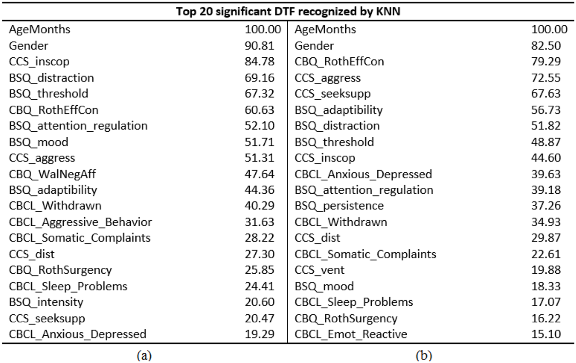
(a) and (b) depicts a list of top 20 important DTFs that significantly contributed to the prediction results during the first and the second approach of implementation of the kNN classifier respectively.

Analysis of the Complexity of Results Produced by the Present Study Against Prior Studies

The results produced by the SEM can be compared with the results of the similar study from the literature (Ajdacic-Gross et al., 2010). The result comparison has been presented in Table 13 which shows that the previous study varies from this one in many respects. For instance, the utilized dataset was not specially prepared for the purpose of investigation on DS; it was a generalized database that was created on male candidates who participated in recruitment camp of the “Swiss Armed Forces in 2003.” Therefore, data samples on the female population who stutter were completely missing. Furthermore, participants’ temperamental traits had not been assessed. Therefore, while performing the path-analysis on risk factors, the author completely missed the temperamental traits of a participant who stuttered.

Table 13.

Analysis of the Complexity of Results Produced by the Present Study Against Prior Studies.

Metrics	The present study	Ajdacic-Gross et al. (2010)
Dataset used	DSP dataset	Swiss Armed Forces in 2003
Subjects’ age group	3–7 years	18–20 years
Aimed for	Analyzing DTFs of children through SEM and machine learning algorithms	Analysis of risk factors concerning stuttering in adults through SEM
Approach used	SEM	SEM
Involved independent variables	DTFs of children including CWS and CWNS	Non-DTFs factors related to birth, education, genetic, siblings, parent habits
Outcomes	The risk factors include gender, age, approach, threshold, adaptability, activity were resulted as background variables.	It relates below risk factors with stuttering: premature birth, probable attention deficit hyperactive disorder, parent’s alcohol abuse, parents and relatives having obsessive-compulsive disorder, having a disabled mother and having a parent from a foreign country.
	The risk-factors like emotional-reactive, anxious-depressed, attention-regulation, and negative-affectivity were resulted as first-level intermediate variables.
	While, other risk factors such as effortful-control, sleep problems, intensity, and coping by venting and distancing were categorized into as Second-level intermediate variables.

Table 14 depicts the present study’s analysis of results was carried out against a prior study. The present study’s results would bring a capability of productivity against new testing data is since the proposed predictive models were trained well on a training set which can be tested anytime over a variety of testing sets.

Table 14.

Analysis of the Complexity of Results Produced by the Present Study Against Prior Studies.

Metrics	The present study	Kefalianos et al. (2017)
Number of data samples	372	173
Subjects’ age group	3–7 years	3–6 years
Aimed for	Predicting the odds of childhood stuttering	Evaluating within groups temperaments of CWS with age 3, 4, and 6
Applied methods	ML-based SVM, RF and kNN	Means, std. deviation
Independent variables	Demographic and temperaments of both CWS and CWNS	Temperaments of mentioned age groups of CWS
Would it bring predictive capacity in the results against unknown sample of children	Yes, SVM, RF and kNN can predict odds of stuttering when the unknown testing set is provided	No, comparing mean and std. deviation cannot add prediction capacity in results against unknown testing set
Prediction accuracy against testing set (%)	Min: 60.98, Max: 95.28	NA
Error %	Min: 04.72, Max: 39.02	NA
Sensitivity %	Min: 41.18, Max: 98	NA

Research Implications, Future Directions, and Limitations

In this research, the authors attempted to propose a conceptual model to investigate the interrelationships among the DTFs with respect to stuttering childhood. Another attempt was made to bring predictive capabilities in the outcomes of childhood stuttering through predictive modeling. Several associates such as Researchers, Psychiatrists, SLPs, and Consultants would benefit from the results of this study. From the researchers’ point of view, by employing a variety of machine learning algorithms, this work can be extended for obtaining even more accurate prediction outcomes. The outcomes of the current study can be equated through the use of other peer datasets concerning childhood stuttering. Furthermore, by taking present research as a reference model, and even more, effective predictive models can be created for an early prognosis of this disorder. It was reported that if CWS receives an early mediation (through early prognosis), then there are 7.7 odds of getting out of their stuttering (Onslow & O’Brian, 2013).

Literature reported that therapists and SLPs are struggling with various content-based problems (Chmela & Johnson, 2018). Specifically, various hindrances are coming across while attempting to determine the key predicting factors attached to the endurance and restoration of stuttering. Also, many difficulties are arising when it comes to handling the behavior and emotions of CWS. Therefore, the findings of this study could support therapists and SLPs in understanding the interrelations among temperamental factors concerning childhood stuttering. Moreover, the top 20 important DTFs generated by the RF and the kNN can be considered as significant contributing risk factors concerning the endurance and restoration from stuttering.

In addition to DTFs, the DSP dataset contains other essential factors that can be involved in model building. For example, the linguistic features of CWS and CWNS can be paired with the DTFs to improve results in future studies. The applied empirical methods can also be used to investigate the role of other psychological and neurological-based predictors in the persistence and recovery of stuttering.

Conclusion

The outcomes of this study showed how the historical data about stuttering is a highly useful source. This data can be utilized to investigate healthcare solutions for individuals who stutter through structural and predictive modeling. The results of the SEM analysis suggest that the structural equation models are efficient in exploring the potential interrelationships among the DTFs in relation to childhood stuttering. Explored interconnections among the DTFs can be useful to understand their direct and indirect effect on persistence and restoration from childhood stuttering. The SEM-based multivariate regression provides the significance level of every background and intermediate variable in relation to the dependent variable through p-values. This regression further provides directionalities of every variable over the dependent variable indicating their positive and negative contribution concerning childhood stuttering. The negative directionality of variables suggests such variables can contribute to the recovery from stuttering. While the variables with positive directionality suggest those variables lead to the persistence of stuttering.

The actual instances of CWS and CWNS were manually recorded in the dataset through a variety of parent-reporting questionnaires. But, the beauty is of predictive models is that they predicted the possible instances of CWS and CWNS against testing data. This finding suggests that those models efficiently captured hidden associations between the DTFs and the dependent variable. Hence, the DTFs can act as significant predictors for predicting possible childhood stuttering. Further, the impact of an imbalanced and balanced DSP was seen in the prediction results. The prediction outcomes improved remarkably when predictive models were trained and tested over the re-sampled version of the DSP dataset. Thus, the present study has delivered an empirical approach through predictive analytics that has the predictive capability to predict future events when it is provided with new data of unseen children. However, the results of this study can be confirmed by validating them against contemporary datasets of stuttering. Thus, the present study’s outcomes and findings provided potential healthcare solutions through applied methods.