Sage Journals: Discover world-class research

Abstract

Green and low-carbon development has become a compelling trend of our time. To formulate policies for development and also reduction of carbon emissions, quantifying the trend of tourism in green sustainable development is an essential issue for China, which is undergoing an economic transformation. This study first measured China’s domestic tourism carbon emissions through a bottom-up approach and then used the robust Granger causality test on annual data from 1993 to 2019 to investigate the relationships among China’s domestic tourism revenue, carbon emissions, and economic growth. The empirical results show that: (1) Carbon emissions of the domestic tourism industry are growing steadily, and the carbon emissions of the transportation industry determine the trend of the total carbon emissions of the domestic tourism industry, (2) long-term equilibrium relationships exist among China’s domestic tourism, carbon emissions, and economic growth, and (3) bidirectional causal relationships among economic growth, carbon emissions, and domestic tourism revenue have been detected with the robust Granger causality test, and the time-varying causal relationships may change markedly in these times of significant events and policy changes. Therefore, policymakers should coordinate the relationships among domestic tourism revenue, carbon emissions, and economic growth, in an effort to promote the development of sustainable tourism in China.

Keywords

domestic tourism demand carbon emissions economic growth VAR model robust Granger causality test

Introduction

As a comprehensive industry in the national economy, tourism has the role of integrating with the development of other economic sectors and improving the structure of the national economy. In addition, tourism plays a crucial role in cultural exchange, expanding domestic demand, stabilizing economic growth, and increasing employment rates (see, e.g., Hesami et al., 2020; Liu & Song, 2018). Therefore, tourism is also known as the engine of a country or region (Brida & Risso, 2009).

China’s tourism industry has developed rapidly since the 1978 launch of the nation’s reform and opening-up. At present, the nation’s domestic tourism market is in a “central position” among the three major tourism markets and plays a pivotal role in economic development (Brida et al., 2020). To demonstrate, China’s total tourism revenue in 1997 was 0.34 trillion Yuan, and in 2019 it reached 6.63 trillion Yuan, 19.5 times that of 1997. Within that overall total, domestic tourism revenue in 1997 was 0.24 trillion Yuan, and in 2019, it reached 5.73 trillion Yuan, 23.88 times that of 1997. According to the “Statistical Communiqué of the Ministry of Culture and Tourism of the People’s Republic of China on Cultural Development in 2019,” the total contribution of tourism to GDP in 2019 was 10.94 trillion CNY, thus accounting for 11.05% of China’s GDP. The number of direct employments related to tourism in 2019 was 28.25 million, while the number of direct and indirect employments related to tourism was 79.87 million, thus accounting for 10.31% of the total employed population in China.

Although tourism can bring substantial social benefits, it can also hurt the environment because most tourist activities require fossil fuel, and the resulting carbon dioxide emissions harm the global climate (Paramati et al., 2017). Katircioglu (2014) took Turkey as an example and found that tourism has led to a significant increase in carbon dioxide emissions, and in terms of human factors, tourism has been shown to be one of the main drivers of global warming (Chen et al., 2018; Gossling, 2013; Gossling & Buckley, 2016). According to data released by the United Nations World Tourism Organization in 2018, the carbon dioxide emissions of the global tourism industry will exceed 6.5 billion tons by 2025. In addition, the carbon dioxide emissions generated by tourism transportation, hotel accommodations, and other tourism activities account for a considerable proportion of the overall carbon emissions from the tourism industry (Jones & Munday, 2007).

The rapid development of China’s domestic tourism industry has brought about a large-scale use of fossil fuels and has resulted in significant carbon dioxide emissions. In recent years, the Chinese government has paid increasing attention to the sustainable development of the economy, and in that light the tourism industry has been encouraged to actively adopt a low-carbon economy to reduce its carbon dioxide emissions (Bing et al., 2010; Lee et al., 2017). Thus, it is crucial to sort out the relationships among tourism, carbon emissions, and economic growth (Carlo, 2014).

Most of the previous literature about the causal relationships among tourism demand, carbon emissions, and economic growth has been based on the Granger causality test under a stable environment (Fonseca & Sanchez-Rivero, 2020a; Khan & Hou, 2020). However, macroeconomic time series data are often unstable (Clark & McCracken, 2006; Stock & Watson, 1996). In addition, the estimated parameters may be varying (Cogley & Sargent, 2005), especially for China during its economic and social transformation. In the wake of China’s reform and opening-up, the nation has also experienced various significant events, including financial crises, natural disasters, public health emergencies, the Olympic Games, and other occurrences. Whether an event’s outcome was good or bad has substantially impacted China’s domestic tourism, carbon emissions, and economic development, and that inevitably will have led to instability in time series data. As shown in Rossi (2005), traditional Granger causality tests may have no power in the presence of instability.

Gunduz and Hatemi (2005) found that the tourism-led growth hypothesis was supported empirically in the case of Turkey. However, with economic development, studies have arrived at contrasting findings—Can and Gozgor (2016) arrived at the opposite conclusion, that the economy-driven tourism growth hypothesis is not supported empirically in Turkey. The traditional Granger causality test results in a stable environment may actually have errors and point toward misleading conclusions. Therefore, simply supporting or not supporting a hypothesis is not a rigorous analysis, because it ignores the fact that the relationships between variables are not immutable, objective laws. Furthermore, it ignores the impact of significant events in the developmental process of changes in the relationships between variables, and naturally, its conclusion is not robust. Especially in the presence of instability, the study of time-varying causality becomes significant. In the process of economic development, the effectiveness of the relationship between tourism and economic growth is crucial for the government’s formulation of tourism and growth policies. Research on the relationship between tourism and carbon emissions is pivotal for coordinating and adhering to the development of a tourism industry that remains green and low-carbon. At the same time, clarifying the relationships among tourism, carbon emissions, and economic growth will help coordinate the green development of tourism and the economy. This study adopted the robust Granger causality test, on the basis of its effectiveness in an unstable environment (Rossi & Wang, 2019), to investigate the relationships among tourism demand, carbon emissions, and economic growth. Our findings significantly contribute to the existing tourism literature.

The rest of this paper proceeds as follows. First, we give a brief overview of the existing literature, and we follow that review with a description of the methodology we used for this study. Next, we present our analyses and the empirical results. Finally, we discuss the findings of the research.

Literature Review

As tourism’s status in economic development continues to increase, the relationship between tourism development and economic growth is a hot topic for research and indeed is becoming a trend in the tourism literature (Wu et al., 2021). However, evidence shows that tourism also has a particular impact on the environment. The large-scale use of fossil fuel in the tourism industry has produced a large amount of carbon dioxide, and that production of greenhouse gas to a certain extent exacerbates the development of global warming (Paramati et al., 2017). Therefore, the carbon dioxide emissions of the tourism industry should first be measured when one is analyzing the effect of tourism on carbon dioxide emissions. There are two main methods for measuring carbon dioxide emissions in the tourism industry: the bottom-up method (Tang & Abosedra, 2014), such as the input-output method (Zhong et al., 2015), and the top-down method (Liu et al., 2018). A large number of studies have gone on to investigate the relationships among tourism, carbon emissions, and economic growth.

In the existing literature, the relationship between tourism and economic growth can be divided into four categories. The first viewpoint supports the tourism-led economic growth hypothesis (TLEGH), which means that tourism can actively promote economic growth. For example, Balaguer and Cantavella-Jorda (2002) used cointegration and causality tests to explore the role of tourism in Spain’s economic development, and their empirical results provided evidence for TLEGH. Gunduz and Hatemi (2005) confirmed that TLEGH is established in Turkey. Gökovali and Bahar (2006) used data from Mediterranean countries from 1987 to 2002 to verify whether TLEGH is a valid hypothesis in that region of the world, and their results showed that tourism has a positive impact on economic growth—thus supporting TLEGH. Croes (2008) explored the relationship between tourism development and economic expansion in Nicaragua and found that tourism development could significantly affect economic expansion. Belloumi (2010) analyzed the role of tourism in Venice’s economic growth and found that tourism positively impacted GDP growth. Lean and Tang (2010) also confirmed the validity and stability of the positive causal relationship between Malaysia’s tourism industry and the country’s economic growth. Tang et al. (2014) found that tourism had made essential contributions to the economic growth of the Middle East and North Africa. Kyophilavong et al. (2018) confirmed that the TLEGH is established in Laos. Mohapatra (2018) investigated the relationship between economic growth and tourism revenues and expenditures in the South Asian Regional Cooperation Alliance, and found that tourism revenue there affected economic growth. Wu and Wu (2018) investigated the causal relationship between international tourism revenue and economic growth in 31 regions of China, and their results provided evidence for the TLEGH in Anhui, Henan, Jiangxi, Jilin, Fujian, Jiangsu, Shandong, Tianjin, Changchun, Inner Mongolia, Qinghai, Tibet, and Yunnan. Balli et al. (2019) took the Mediterranean region as an example and found that the TLEGH was valid there. Shehzad et al. (2019) determined that tourists make up an important share in China’s economic growth. Wu and Wu (2019) provided evidence for the TLEGH in Cambodia, China, and Malaysia. Fonseca and Sanchez-Rivero (2020b) believed that the higher the acceptance of the TLEGH is, the higher its tourism specialization and larger its population size will be.

The second viewpoint about tourism and economic growth supports the economy-driven tourism growth hypothesis (EDTGH), which suggests that economic growth affects tourism development. Oh (2003) analyzed the relationship between South Korea’s economic growth and tourism, and the results provided evidence for EDTGH. Payne and Mervar (2010) used the data of Croatia from the first quarter of 2000 to the third quarter of 2008 to test whether EDTGH was established there and found a positive causal relationship between real GDP and international tourism revenue, thus supporting the EDTGH. Rivera (2017) found tourism growth to be a product of economic growth. Wu and Wu (2018, 2019) provided evidence for the EDTGH in regions such as Hubei, Hunan and Hong Kong SAR in China, and in Hong Kong, Indonesia, the Philippines, and South Korea.

The third viewpoint supports both the TLEGH and the EDTGH and posits that a bidirectional causal relationship exists between tourism and economic growth. Dritsakis (2004) investigated the relationship between Greece’s real GDP and the nation’s international tourism revenue and found that the TLEGH was significant, while the EDTGH was less significant. Lee and Chien (2008) found a bidirectional causal relationship between global tourism revenue and the number of international tourist arrivals in Taiwan. Jebli and Hadhri (2018) investigated the relationship between international tourism and economic growth in the top 10 tourist countries and found a bidirectional causal relationship between international tourism and economic growth.

The fourth viewpoint on tourism and economic growth holds that there is no causal relationship whatsoever between tourism and economic growth. Wu and Wu (2018) found that neither the TLEGH nor the EDTGH was supported in Heilongjiang, Shanxi, Beijing, Guangdong, Hainan, Liaoning, Shanghai, Zhejiang, Gansu, Guangxi, Guizhou, Ningxia, Sichuan, and Xinjiang in China. Katircioglu (2009) found no relationship of cointegration between international tourism and economic growth, and the Granger causality tests for the TLEGH and EDTGH were not valid in Turkey. Brida et al. (2011) used the traditional Granger causality test, and they too found no Granger causality between tourism and economic growth from 1965 to 2007 in Brazil.

Nowadays, in the midst of such varied data, more and more research is focusing on the green economy and sustainable tourism development. Therefore, clarifying the causal relationships among tourism demand, carbon emissions, and economic growth is essential for formulating optimal policies for tourism and economic development. Becken and Simmons (2002) found that certain tourism activities in New Zealand used a lot of fossil fuel, and the resulting carbon dioxide contributed to global warming. Becken and Patterson (2006) argued that the tourism industry requires a large amount of fossil fuels, and that is an essential source of carbon dioxide emissions. Fodha and Zaghdoud (2009) found a one-way causal relationship from Tunisian income to pollution, with the income causing environmental changes in the short and long term. Al-mulali (2011) found that carbon dioxide emissions and fuel consumption have had a long-term association with economic growth in the Middle East and North Africa. Dogan and Aslan (2017) analyzed the relationships among carbon dioxide emissions, actual income, energy consumption, and tourism in the EU countries during the period 1995 to 2011, and found a unidirectional causal relationship from tourism to carbon emissions. Danish and Wang (2018) argued that although tourism significantly promotes economic growth, it also reduces environmental quality. Liu et al. (2019) found that GDP can generate both carbon dioxide emissions and tourism income and had no significant impact on the environment. Akadiri et al. (2019) and Udemba (2019) investigated the Granger causalities between Turkey’s actual income, globalization, environment, and tourism, based on the Vector Error Correction Model (VECM), and found that real income and globalization Granger-caused CO₂ emissions in the long run. Lee and Brahmasrene (2013) used EU panel data from 1988 to 2009 to investigate the impact of tourism on economic growth and carbon dioxide emissions and found that tourism income contributed to economic growth, as well as to the increase in carbon dioxide emissions. Kasman and Duman (2015) investigated the relationship between carbon dioxide emissions and economic growth in EU countries and found an essential connection between carbon emissions and economic growth.

The validity and stability of the relationships among tourism, CO₂ emissions, and the economy are essential for policymakers in formulating appropriate tourism and growth policies. In the latest research on the relationship between tourism and environmental pollution, Chishti et al. (2020) and Nosheen et al. (2021) found that tourism increased carbon dioxide emissions, thereby reducing environmental quality, which was the same as Dogan and Aslan’s (2017) conclusion but contrary to the conclusion of Liu et al. (2019). The latest research on the relationship between tourism and economics also supports the validity of the tourism-led growth hypothesis. For example, Lee’s (2021) results empirically demonstrated that international tourism revenues significantly contributed to economic growth. Considering the possibility that the causality may be unstable, some scholars have introduced a time-varying Granger causality test. Among them, Tang and Tan (2013) used the recursive Granger test method to verify that the relationship between tourism and economic growth was unstable in different types of countries. Still, this method fails to take into account the impact of instability on causality.

In short, the causality test results regarding relationships among tourism, carbon emissions, and economic growth are different when based on the traditional Granger causality test under stable conditions versus when they are based on other Granger causality tests. That said, the relationships among the variables are not static in reality because of the complexity and instability of macroeconomics. So far, the above questions have not been solved using the traditional Granger causality test, especially in China, which is in a period of economic transformation and is especially vulnerable to unstable factors. This paper uses the latest developed econometrics method to more effectively investigate the correlations between tourism, carbon emissions, and economic growth in an unstable environment.

Methodology

Evidence shows that the sign and the size of the estimated parameters based on the vector autoregression (VAR) model will change substantially over time—that is, the instability parameter results will lead to different outcomes at different times from the Granger causality tests (Rossi, 2005). Therefore, we have used the robust Granger causality test proposed by Rossi and Wang (2019) to analyze the relationships among China’s domestic tourism, its carbon emissions, and its economic growth, and compared the results with those from the traditional Granger test. We started with a VAR model to present the robust Granger causality test, with the conventional VAR having the following form:

y_{t} = Φ_{1} y_{t - 1} + Φ_{2} y_{t - 2} + \dots + Φ_{p} y_{t - p} + ε_{t},

(1)

where $y_{t} = {[y_{1, t}, y_{2, t}, \dots, y_{n, t}]}^{'}$ is an $n \times 1$ vector and $Φ_{t}$ is the coefficient matrix, $t = 1, 2, ..., T$ . $ε_{t}$ is the error, and $ε_{t} ~ i . i . d . N (0, 1)$ .

For the possibility of parameter instability, robust Granger causality tests are used to consider various forms of instability, so they are a more general case of testing possible nonlinear restrictions on models fitted with the generalized method of moments, and tests on subsets of parameters. Let $ϕ_{t}$ change at some unknown point in time $τ : ϕ_{t} = ϕ_{1} (t \leq τ) + ϕ_{2} (t > τ)$ . Let ${\hat{ϕ}}_{1 τ}$ and ${\hat{ϕ}}_{2 τ}$ denote the OLS estimators before and after the break. The significance of the predictors and their stability over time is tested by a joint test method proposed by Rossi (2005). The null hypothesis proposes that there is no Granger causality at any point in time—that is, $H_{0} : ϕ_{t} = ϕ = 0$ . The robust Granger test builds on two components: $(τ / T) {\hat{ϕ}}_{1 τ} + {1 - (τ / T)} {\hat{ϕ}}_{2 τ}$ and ${\hat{ϕ}}_{1 τ} - {\hat{ϕ}}_{2 τ}$ . According to Rossi and Wang (2019), a test on whether the first component (the full-sample estimate of the parameter) is zero detects situations in which the parameter is constant and different from zero. A test on whether the second component (the difference between the parameters estimated in the two subsamples) is zero detects situations in which the parameter changes.

Taking the VAR(2) model as an example, we can model China’s domestic tourism revenue (TR), carbon emissions (CO₂), and gross domestic product (GDP) and obtain the following equation (2).

[\begin{matrix} T R_{t} \\ G D P_{t} \\ C O_{2, t} \end{matrix}] = Φ_{1} [\begin{matrix} T R_{t - 1} \\ G D P_{t - 1} \\ C O_{2, t - 1} \end{matrix}] + Φ_{2} [\begin{matrix} T R_{t - 2} \\ G D P_{t - 2} \\ C O_{2, t - 2} \end{matrix}] + [\begin{matrix} ε_{t}^{T R} \\ ε_{t}^{G D P} \\ ε_{t}^{C O_{2}} \end{matrix}] .

(2)

The coefficients of the traditional Granger causality test based on the VAR(2) model are as follows:

Φ_{j} = [\begin{matrix} Φ_{j}^{(T R, T R)} & Φ_{j}^{(T R, G D P)} & Φ_{j}^{(T R, C O_{2})} \\ Φ_{j}^{(G D P, T R)} & Φ_{j}^{(G D P, G D P)} & Φ_{j}^{(G D P, C O_{2})} \\ Φ_{j}^{(C O_{2}, T R)} & Φ_{j}^{(C O_{2}, G D P)} & Φ_{j}^{(C O_{2}, C O_{2})} \end{matrix}], j = 1, 2, ...

(3)

Therefore, if the null hypothesis of the traditional Granger causality test $H_{0}^{*} : Φ_{1} = Φ_{2} = 0$ holds, it means that the explanatory variable is not the Granger cause for the explained variable. For example, carbon emissions do not Granger-cause domestic tourism revenue, if and only if equation (4) holds:

Φ_{1}^{(T R, C O_{2})} = Φ_{2}^{(T R, C O_{2})} = 0 .

(4)

For the robust Granger causality test, the specification of VAR with time-varying parameters is:

[\begin{matrix} T R_{t} \\ G D P_{t} \\ C O_{2, t} \end{matrix}] = Φ_{1, t} [\begin{matrix} T R_{t - 1} \\ G D P_{t - 1} \\ C O_{2, t - 1} \end{matrix}] + Φ_{2, t} [\begin{matrix} T R_{t - 2} \\ G D P_{t - 2} \\ C O_{2, t - 2} \end{matrix}] + [\begin{matrix} ε_{t}^{T R} \\ ε_{t}^{G D P} \\ ε_{t}^{C O_{2}} \end{matrix}],

(5)

where the time-varying coefficient matrix is as follows:

\begin{array}{l} Φ_{j, t} = [\begin{matrix} Φ_{j, t}^{T R, T R} & Φ_{j, t}^{T R, G D P} & Φ_{j, t}^{T R, C O_{2}} \\ Φ_{j, t}^{G D P, T R} & Φ_{j, t}^{G D P, G D P} & Φ_{j, t}^{G D P, C O_{2}} \\ Φ_{j, t}^{C O_{2}, T R} & Φ_{j, t}^{C O_{2}, G D P} & Φ_{j, t}^{C O_{2}, C O_{2}} \end{matrix}], j = 1, 2; \\ t = 1, 2, ..., T \end{array}

(6)

The null hypothesis of the robust Granger causality test is $H_{0} : Φ_{1, t} = Φ_{2, t} = 0$ . For example, carbon emissions do not Granger-cause domestic tourism revenue, if and only if equation (7) holds:

Φ_{1, t}^{T R, C O_{2}} = Φ_{2, t}^{T R, C O_{2}} = 0 .

(7)

Moreover, there are four test statistics for the robust Granger causality test (Rossi, 2005): the ExpW* (the exponential Wald), the MeanW* (the mean Wald), the Nyblom* (the Nyblom) test statistics (Nyblom, 1989), and the QLR* (the Quandt likelihood-ratio) test statistic (Andrews, 1993). Rossi and Wang (2019) had shown that the robust Granger causality test is more effective than the traditional Granger causality test in the presence of instability. More importantly, the time-series graph of Wald statistics with 5% and 10% critical values as the significance levels generated by the robust Granger causality test can also find the time point of the emergence and disappearance of the Granger causal relationship.

Results and Discussion

Data Sources

In our study, we used data for the years from 1993 to 2019 and with the variables all taking the natural logarithm. We selected domestic tourism revenue (TR) to represent the variable of domestic tourism and abbreviated it as LNTR, we chose domestic tourism carbon emissions (CO₂) to represent the variable for carbon emissions and abbreviated it as LNCO₂, and we selected gross domestic product (GDP) to represent the variable for economic growth and abbreviated it as LNGDP.

The data source of passenger turnover and domestic tourists was from the China Statistical Yearbook, compiled by the China National Bureau of Statistics, from 1994 to 2020. Revenue data of various star-rated hotels and domestic tourism came from various issues of the “China Tourism Statistical Yearbook (1994–2020),” compiled by the National Tourism Administration. The statistical data of the scale of various tourism activities came from the “Tourism Sample Survey Information (2001–2020)” issued by the Policy and Regulations Department of the National Tourism Administration.

According to previous literature studies, the proportion of railways is 32.7%, that of highways is 27.9%, that of waterways is 10.6%, and that of civil aviation is 36.7%. Their corresponding unit carbon emissions are 27, 133, 106, and 137 g/km, respectively. Respective energy consumption coefficients for five-star to one-star hotels are 155, 130, 110, 70, and 40 MJ per night, and the hotel’s carbon dioxide emission coefficient is 43.2 gC/MJ. For sightseeing, carbon dioxide emissions are 417 gC/person; for leisure and vacation, 1,670 gC/person; for business meetings, 786 gC/person; for visiting relatives and friends, 591 gC/person, and for other tourist activities 172 gC/person (available at China Travel Cities Web Reputation report), respectively.

Estimation of CO₂ Emissions From the Domestic Tourism Industry

There are two commonly used methods to measure CO₂ emissions: the top-down method, and the bottom-up method. The top-down approach is used to measure the CO₂ emissions of the domestic tourism industry and is based on China’s basic domestic tourism data. The calculation is divided into three parts: the CO₂ produced by tourism transportation, the CO₂ produced by hotel accommodations, and the CO₂ produced by tourism activities. The results of these three parts are summed to arrive at the final carbon dioxide emissions of the tourism industry. The specific formula is shown in equations (8) and (9):

{CO}_{2} = C O_{2, T} + C O_{2, H} + C O_{2, A},

(8)

\begin{array}{l} {CO}_{2} = \sum_{i = 1}^{4} λ N_{i} D_{i} e_{i t} + 365 \times \sum_{j = 1}^{5} B_{j} P_{j} e T_{e j} \frac{1}{1000} \times \frac{44}{12} + \\ \sum_{k = 1}^{5} M_{k} W_{k} P_{c k}, \end{array}

(9)

where, CO₂ is the total amount of carbon dioxide emissions from the domestic tourism industry, CO_2,T indicates the CO₂ emissions of travel−related transportation, CO_2,H represents the emissions from hotel accommodations, and CO_2,A represents the emissions from activities. The value of λ is the proportion of tourists who choose to travel, which includes by civil aviation, highways, railways, and waterways; N_i represents the total number of tourists who choose travel mode i (civil aviation, highways, railways, and waterways); D_i is the travel distance of travel mode i; $N_{i} D_{i}$ indicates the passenger turnover of transportation mode i; $e_{i t}$ (g/pkm) indicates the unit emissions of carbon dioxide for transportation mode i; $B_{j}$ represents the number of beds in the star-rated hotels, and $P_{j}$ is the annual accommodation rate of the star-rated hotels; e is the carbon dioxide emission coefficient per night; $T_{e j}$ is the energy consumption coefficient of the hotel per night, and 1/1,000 is the unit conversion coefficient; 44/12 indicates the ratio of the molecular weight of CO₂ to the atomic weight of B; $M_{k}$ is the number of tourists; $W_{k}$ is the proportion of tourists choosing the activity type (sightseeing, leisure vacation, business meetings, visiting relatives and friends, and others); and $P_{c k}$ is the CO₂ emissions per unit of the activity types.

Figure 1 shows that the total carbon dioxide emissions in the domestic tourism industry have undergone exponential growth, especially from 2004 to 2012. The total carbon dioxide emissions of the domestic tourism industry have increased rapidly. The average annual growth rate of total CO₂ emissions of domestic tourism is 171.26%, the amount of emissions in 2004 was 7,446 × 10⁴ t, and in 2012 the emissions had reached 15,399 × 10⁴ t. The carbon emissions of the tourism transportation industry have been the main source of domestic tourism carbon emissions and tend to track consistently with the total carbon emissions of domestic tourism.

Figure 1.

CO₂ emissions from China’s domestic tourism from 1993 to 2019 (unit: 10⁴ t).

Variable Descriptive Analysis and the Unit Root Test

Figure 2(a) shows that domestic tourism carbon emissions, tourism revenue, and economic growth generally have the same trend, whereas the volatility of domestic tourism revenue is more significant because it is vulnerable to essential events, such as sudden public health events and financial crises. The same phenomena also can be seen in Figure 2(a), with domestic tourism revenue having fluctuated significantly during the SARS epidemic in 2003.

Figure 2.

Time series of domestic tourism revenue, carbon emissions, and economic growth: (a) raw data timing diagram (1993–2019) and (b) first-order differential data timing diagram (1994–2019).

In kurtosis statistics, domestic tourism carbon emissions, economic growth, and domestic tourism revenue data all have an apparent low kurtosis distribution, with a slight fluctuation in depth, and the average representation is relatively poor. In terms of skewness statistics, the skewness coefficients of the three variables tend to zero, which means that the data tend to be symmetrical. From the Jarque–Bera (J–B) statistics of the three variables, as given in Table 1, it can be seen that the three variables are all subject to a normal distribution.

Table 1.

Descriptive Analysis Results.

Variables	Observed	Mean	Variance	Skewness	Kurtosis	J–B statistics
LNCO₂	27	8.97	0.62	−0.32	1.65	2.51
LNGDP	27	12.32	1.01	−0.09	1.71	1.88
LNTR	27	8.91	1.28	0.09	1.81	1.63

Note. The sample period was from 1993 to 2017. J–B statistics = Jarque-Bera statistics.

We further investigated the stationarity of the three variables. Figure 2(a) shows a clear growth trend in the domestic tourism carbon emissions, tourism revenue, and economic growth. Figure 2(b) shows that the first-order differential variables, abbreviated as DLNCO₂, DLNTR, and DLNGDP, tended to be stable. We used the Augmented Dickey–Fuller (ADF) test method to perform a unit root test on the variables. We determined the optimal lag order according to the minimum criteria of the Akaike Information Criterion (AIC) and the Schwartz Information Criterion (SIC). The unit-roots test results, listed in Table 2, show that the three first-order differential variables were all stationary series.

Table 2.

ADF Tests Results.

Variables	(c, t, k)	Critical values			t-statistics	p-Value
Variables	(c, t, k)	1%	5%	10%	t-statistics	p-Value
LNCO₂	(c, t, 2)	−4.35	−3.59	−3.23	−0.66	.96
LNTR	(c, t, 2)	−4.35	−3.59	−3.23	−1.85	.65
LNGDP	(c, t, 2)	−4.37	−3.60	−3.23	−2.28	.42
DLNCO₂	(c, 0, 2)	−3.72	−2.98	−2.63	−5.34	.00***
DLNTR	(c, 0, 2)	−4.37	−3.60	−3.23	−4.96	.00***
DLNGDP	(c, 0, 2)	−4.37	−3.60	−3.23	−3.49	.06*

Note. *** and * denote significance at the 1% and 10% levels, respectively. For the (c, t, k), c represents the intercept term, t represents the trend term, 0 means that the trend term is not included, and k represents the lag order.

VAR Models and the Johansen Cointegration Test

It was important to know whether a long-term equilibrium relationship existed between any of the variables before the Granger causality test, so we adopted the Johansen cointegration test to investigate the long-term equilibrium relationships among LNCO₂, LNTR, and LNGDP. The results in Table 3 show a cointegration relationship among the three variables; therefore, we used logarithm values for the raw data to construct a VAR model for examining the relationships among tourism development, economic growth, and carbon dioxide emissions.

Table 3.

Johansen Cointegration Test Results.

Null hypothesis	Eigenvalue	Trace statistics	5% critical value	p-Value
None	0.71	48.04	42.91	.01**
At most 1	0.34	16.34	25.87	.46
At most 2	0.20	5.62	12.51	.50

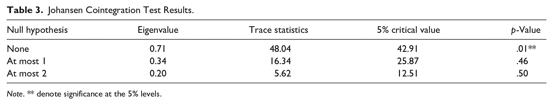
Note. ** denote significance at the 5% levels.

It is crucial to choose the correct lag period for the VAR model when investigating the dynamic relationships among variables. We chose the optimal lag order of the VAR model according to six criteria, including the AIC criterion and SIC criterion, and we list the results in Table 4.

Table 4.

Selection Criteria for Lag Length of the VAR Model.

Lag	LogL	LR	FPE	AIC	SIC	HQIC
0	8.11	NA	0.00	−0.42	−0.27	−0.38
1	113.90	188.95	2.03e-08*	−9.12	−8.53*	−8.97*
2	120.01	5.61	3.51e-08	−8.70	−7.61	−8.26
3	133.93	17.39*	2.21e-08	−9.36*	−7.58	−8.59

Note. LogL = log-likelihood; LR = likelihood ratio; FPE = Final prediction error; AIC = Akaike information criterion; SIC = Schwarz information Criterion; HQIC = Hannan-Quinn information criterion.

Indicates lag order selected by the criterion.

From the results of Table 4, the optimal lag order was finally determined to be 1. The VAR(1) can accurately and effectively reflect the dynamic relationships among domestic tourism carbon emissions, tourism revenue, and economic growth. Therefore, the final VAR(1) model can be shown as follows:

[\begin{matrix} L N T R_{t} \\ L N G D P_{t} \\ L N C O_{2 t} \end{matrix}] = Φ_{1} [\begin{matrix} L N T R_{t - 1} \\ L N G D P_{t - 1} \\ L N C O_{2 t - 1} \end{matrix}] + [\begin{matrix} ε_{t}^{L N T R} \\ ε_{t}^{L N G D P} \\ ε_{t}^{L N C O_{2}} \end{matrix}] .

(10)

The coefficient matrix $Φ_{1}$ has two expressions according to the traditional and robust Granger causality tests, where formula (11) is the coefficient matrix based on the conventional Granger causality test:

Φ_{1} = [\begin{matrix} Φ_{1}^{L N T R, L N T R} & Φ_{1}^{L N T R, L N G D P} & Φ_{1}^{L N T R, L N C O_{2}} \\ Φ_{1}^{L N G D P, L N T R} & Φ_{1}^{L N G D P, L N G D P} & Φ_{1}^{L N G D P, L N C O_{2}} \\ Φ_{1}^{L N C O_{2}, L N T R} & Φ_{1}^{L N C O_{2}, L N G D P} & Φ_{1}^{L N C O_{2}, L N C O_{2}} \end{matrix}],

(11)

and the following formula is the coefficient matrix based on the robust Granger causality test: $Φ_{1, t} = [\begin{matrix} Φ_{1, t}^{L N T R, L N T R} & Φ_{1, t}^{L N T R, L N G D P} & Φ_{1, t}^{L N T R, L N C O_{2}} \\ Φ_{1, t}^{L N G D P, L N T R} & Φ_{1, t}^{L N G D P, L N G D P} & Φ_{1, t}^{L N G D P, L N C O_{2}} \\ Φ_{1, t}^{L N C O_{2}, L N T R} & Φ_{1, t}^{L N C O_{2}, L N G D P} & Φ_{1, t}^{L N C O_{2}, L N C O_{2}} \end{matrix}] .$

For example, if the null hypothesis $H_{0}^{a} : Φ_{1}^{L N T R, L N C O_{2}} = 0$ holds, the traditional Granger causality test believes that carbon emissions do not Granger-cause domestic tourism revenue. On the other hand, if the null hypothesis $H_{0}^{b} : Φ_{1, t}^{L N T R, L N C O_{2}} = 0$ holds, the robust Granger causality test believes that carbon emissions do not Granger-cause domestic tourism revenue. The other null hypothesis had similar forms to the above null hypotheses.

Traditional Granger Causality Tests

Table 5 shows the traditional Granger causality test results for the variables LNCO₂, LNTR, and LNGDP. The results show that there was no Granger causality between domestic tourism revenue and carbon emissions, whereas economic growth was the Granger-cause of domestic tourism revenue—meaning that the EDTGH holds in China. In addition, carbon emissions from domestic tourism were the Granger-cause for economic growth, which shows to a certain extent that tourism energy consumption has played an essential role in economic growth.

Table 5.

The Traditional Granger Causality Test Results.

Null hypothesis	p-Value	Results
LNCO₂ does not Granger-cause LNTR	.30	Accept
LNTR does not Granger-cause LNCO₂	.39	Accept
LNTR does not Granger-cause LNGDP	.10	Accept
LNGDP does not Granger-cause LNTR	.01**	Reject
LNGDP does not Granger-cause LNCO₂	.87	Accept
LNCO₂ does not Granger-cause LNGDP	.02**	Reject

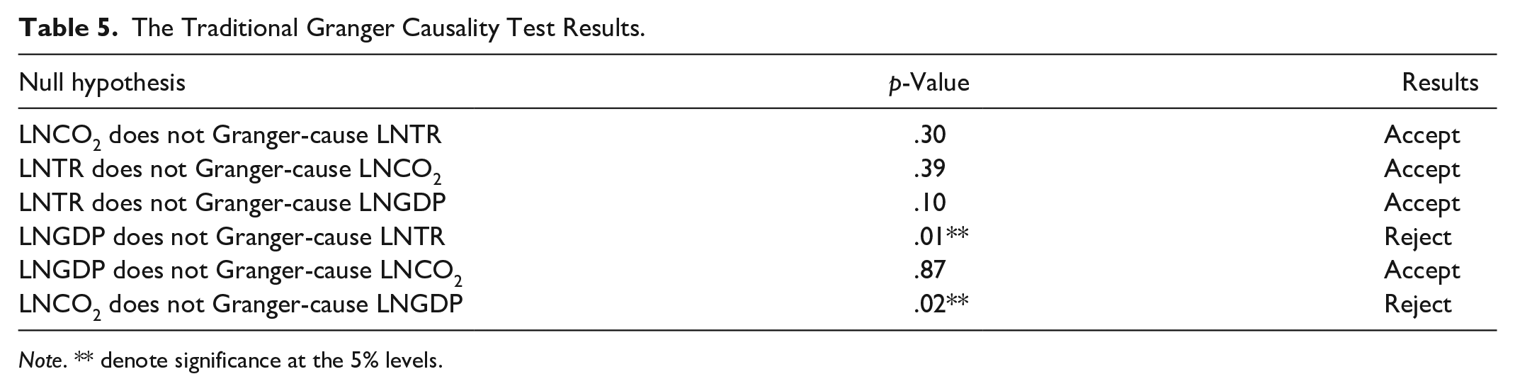
Note. ** denote significance at the 5% levels.

Robust Granger Causality Tests

We used the robust Granger causality test to explore the causal relationships among LNCO₂, LNTR, and LNGDP, and four built-in robust Granger causality test statistics are shown in Table 6.

Table 6.

Results of the Robust Granger Causality Test with Four Test Statistics.

Null hypothesis	p-Value	Null hypothesis	p-Value
A. The causal relationship between tourism carbon emissions and domestic tourism revenue
$L N C O_{2} ↛ L N T R$	$[\begin{matrix} 0.00 & 0.08 \\ 0.00 & 0.00 \end{matrix}]$	$L N T R ↛ L N C O_{2}$	$[\begin{matrix} 0.03 & 0.12 \\ 0.00 & 0.02 \end{matrix}]$
B. The causal relationship between domestic tourism revenue and economic growth
$L N T R ↛ L N G D P$	$[\begin{matrix} 0.03 & 0.16 \\ 0.00 & 0.02 \end{matrix}]$	$L N G D P ↛ L N T R$	$[\begin{matrix} 0.00 & 0.00 \\ 0.00 & 0.00 \end{matrix}]$
C. The causal relationship between economic growth and domestic tourism carbon emissions
$L N G D P ↛ L N C O_{2}$	$[\begin{matrix} 0.04 & 0.19 \\ 0.00 & 0.03 \end{matrix}]$	$L N C O_{2} ↛ L N G D P$	$[\begin{matrix} 0.00 & 0.04 \\ 0.00 & 0.00 \end{matrix}]$

Note. p-Value matrix = $[\begin{matrix} E x p W * & M e a n W * \\ N y b l o m * & Q L R * \end{matrix}]$ , $A ↛ B$ means A does not Granger-cause B.

The causal relationship between LNTR and LNCO₂ in the robust Granger-causality tests

The empirical conclusions differed when we used the robust Granger-causality test instead of the traditional Granger-causality test, as shown in Tables 5 and 6. There was no causal relationship between tourism revenue and domestic tourism carbon emissions in the standard Granger-causality test, but the results were different when we used the robust Granger-causality test.

For the null hypothesis that domestic tourism carbon emissions do not Granger-cause tourism revenue ( $L N C O_{2} ↛ L N T R$ ): Domestic tourism carbon emissions do Granger-cause tourism revenue at the 1% significance level in the robust Granger-causality test, according to the ExpW*, Nyblom*, and QLR* statistics, and for MeanW* statistic the conclusion was significant at the 10% level.

For the null hypothesis that tourism revenue do not Granger-cause domestic tourism carbon emissions ( $L N T R ↛ L N C O_{2}$ ): The p-value in panel A shows that the four built-in test statistics, the ExpW* statistic, the MeanW* statistic, the Nyblom* statistics, and the QLR* statistic, were 0.03, 0.12, 0.00, and 0.02, respectively. The null hypothesis was rejected at the 5% significance level except with the Nyblom* statistic, which means that domestic tourism carbon emissions were the Granger-cause of tourism revenue.

Figure 3 further analyzes the changes in the causal relationship between tourism revenue and domestic tourism carbon emissions over time, using the whole sequence of the Wald statistics across time. Figure 3(a) shows that the entire series of the Wald statistics was below the 5% critical value line most of the time, except for 2008 and 2009, which means that the domestic tourism carbon emissions were the Granger-cause of tourism income in 2008 and 2009 because the Wald statistic fell into the rejection range. The results indicate that the tourism industry is susceptible to significant events. For example, the fact that the 2008 Summer Olympics in China brought huge tourism hotspots to the domestic tourism industry should be the main reason that the domestic carbon emissions Granger-caused tourism revenue becomes significant. In Figure 3(b), the sequence of the Wald statistic was below the line 10% critical value most of the time, except for 1998, which means that tourism revenue did Granger-cause domestic tourism carbon emissions in 1998, and the rest of the sample all accepts the null hypothesis. The results show that rapid economic development has promoted the development of domestic tourism, but that such promotion has been at the cost of carbon emissions since the 1990s. The Wald statistics also indicate that tourism revenue was not the Granger cause for domestic tourism carbon emissions after 2000, because the results all fell into the acceptance region. It was revealed that a low-carbon tourism economy has gradually become the consensus of all sectors of society, and more and more attention is being paid to the energy consumption and environmental pollution caused by tourism.

Figure 3.

The sequence of Wald statistics for the causal relationship between LNTR and LNCO₂: (a) LNCO2 ↛ LNTR and (b) LNTR ↛ LNCO₂.

In summary, the causal relationship between domestic tourism revenue and carbon dioxide emissions varies across time. The significant causal relationship detected between domestic tourism revenue and carbon dioxide emissions was not synchronized and affected by significant events and changes in national policies, and only the one-way causal relationship could be found in the specific time period.

The causal relationship between LNTR and LNGDP in the robust Granger-causality tests

Tables 5 and 6 also show a significant difference between the robust Granger-causality tests and the traditional Granger causality, when investigating the causal relationship between tourism revenue and economic growth.

For the null hypothesis that domestic tourism revenue does not Granger-cause economic growth ( $L N T R ↛ L N G D P$ ): The results reject the null hypothesis, based on the p-value in Table 6, because the four built-in test statistics—ExpW*, MeanW*, Nyblom*, and QLR* statistics—were 0.03, 0.16, 0.00, and 0.02, respectively. We further analyzed the changes in causality over time, using the Wald statistic time series, for critical values of 5% and 10%, as shown in Figure 4(a). The Wald statistics from most years fell in the acceptable domain, and only the Wald statistics from 1996 and 2012 fell in the rejection domain. Generally speaking, then, the Granger-cause relationship from domestic tourism revenue to economic growth was not significant all of the time in China.

For the null hypothesis that economic growth does not Granger-cause domestic tourism revenue ( $L N G D P ↛ L N T R$ ): As shown in Table 6, the p-values of the four built-in test statistics all rejected the null hypothesis at the 1% significant level, which shows that economic growth is the Granger-cause for the domestic tourism revenue in China. We further analyzed the changes in causality over time, using the Wald statistic time series, with critical values of 5% and 10%, as shown in Figure 4(b). The Wald statistics all fell into the rejection domain in the sample period, which means that economic growth was the Granger-cause of the domestic tourism revenue during that time.

Figure 4.

Distribution of Wald statistics of the causal relationship between tourism income and economic growth: (a) the distribution diagram of the Wald statistic representing the null hypothesis that tourism revenue does not Granger-cause economic growth and (b) the distribution diagram of the Wald statistic representing the null hypothesis that economic growth does not Granger-cause tourism revenue.

The causal relationship between LNGDP and LNCO2 in the Granger-causality robust tests

For the null hypothesis that economic growth does not Granger-cause domestic tourism carbon emissions: As is shown in Table 6, the p-values of the four built-in test statistics—ExpW*, MeanW*, Nyblom*, and QLR* statistics—were 0.04, 0.19, 0.00, and 0.03, respectively. At the 10% significance level, the ExpW* statistics, Nyblom* statistics, and QLR* statistics rejected the null hypothesis, while the MeanW* statistics accepted the null hypothesis. We further analyzed the changes in causality over time from the Wald statistic time series, with critical values of 5% and 10%, as shown in Figure 5(a). Generally speaking, economic growth was the Granger-cause of the domestic tourism carbon emissions, but it was not significant, which means that the domestic tourism carbon emissions did not depend on economic growth. We also found that the Wald statistics of the null hypothesis that economic growth does not Granger-cause domestic tourism carbon emissions were rejected most of the time, as shown in Figure 5(a). However, economic growth did Granger-cause the domestic tourism carbon emissions in 1998.

For the null hypothesis that domestic tourism carbon emissions do not Granger-cause economic growth: As shown in Table 6, the p-value of the four built-in test statistics rejected the null hypothesis at the 1% significant level, which shows that domestic tourism carbon emissions are the Granger-cause for economic growth in China. We further analyzed the changes in causality over time, from the time-varying Wald statistic, with critical values of 5% and 10%, as shown in Figure 5(b). The causal relationship fluctuated significantly over time. The Wald statistics in 1996 and 2012 fell into the rejection domain, which means the domestic tourism carbon emissions were the Granger-cause of economic growth in those years. The economic growth was due to domestic tourism carbon emissions to a certain extent, and the Granger relationship in other years was not significant.

For the robust Granger test analytic results, the readers are referred to Table 6 and Figures 3 through 5. The results confirm that economic growth Granger caused tourism, which is consistent with the tourism-led growth hypothesis supported by Payne and Mervar (2010) and Rivera (2017). In contrast, Wu and Wu (2019) and Fonseca and Sanchez-Rivero (2020b) found that the tourism-led growth hypothesis was not supported. In comparing those conflicting findings, the difference may be explained by the fact that our research concluded the tourism-led growth hypothesis only appeared at a particular time node. Meanwhile, our research results confirmed that the relationship between tourism and economic development is time-varying—that is, the causal relationship between tourism development and economic growth varies over time and will be affected by special events.

Figure 5.

Distribution of Wald statistics of the causal relationship between domestic tourism carbon emissions and economic growth: (a) the distribution diagram of the Wald statistic representing the null hypothesis that economic growth does not Granger-cause domestic tourism carbon emission and (b) the distribution diagram of the Wald statistic representing the null hypothesis that domestic tourism carbon emissions do not Granger-cause economic growth.

The study’s results confirm that the Granger relationship between tourism revenue and carbon emissions is only established at a certain point in time, which is different from the decline in environmental quality caused by tourism development supported by the findings of Danish and Wang (2018). A possible explanation would be that carbon emissions are measured in different ways. We calculated carbon emissions on a smaller scale and re-examined whether domestic tourism revenue comes at the cost of carbon emissions. The carbon emissions from domestic tourism were only a tiny part of China’s total carbon emissions, so it is not difficult to explain the conclusion that the relationship between carbon emissions and economic growth was not significant in this study. That relationship differs from the critical relationship between economic growth and environmental pollution, supported by the findings of Fodha and Zaghdoud (2009) and Kasman and Duman (2015). Thus, our empirical results provide new evidence for the influence of uncertainty on the causality of variables and find that the causal relationship between variables is correlated in a trend and is not synchronized in time. Those findings are more novel than the conclusions of previous research and provide new insights for the government on the relationships among tourism, carbon emissions, and economic growth.

All in all, the traditional Granger causality test method differs significantly from the robust Granger causality test method in investigating the relationships among China’s domestic tourism revenue, carbon emissions, and economic growth. That difference occurs because the causal relationships among variables and the instability of economic development will change over time. Specific causal relationships among variables may appear only occasionally, so the traditional Granger causality test cannot detect them. In short, the results of the relationships among tourism, carbon emissions, and economic growth will be different in future research when we use other proxy variables, sample sizes, and research methods.

Conclusions

China’s domestic tourism industry has developed rapidly, and its economic and social roles have become increasingly important since the reform and opening-up. In recent years, the low-carbon tourism economy has become a model for new development. Therefore, it is crucial to accurately analyze the relationships among domestic tourism, carbon emissions, and economic development, because those relationships are important for the government and other relevant departments in formulating policies for green and sustainable development.

This paper first measured the carbon emissions of China’s domestic tourism industry through the bottom-up method, building a VAR model with the annual domestic tourism revenue, carbon emissions, and economic growth data, and employing the robust Granger causality test method to investigate the relationships among China’s domestic tourism, carbon emissions, and economic growth.

We found that the economy-driven tourism growth hypothesis is supported empirically in China, meaning that economic development in China plays an essential role in driving the development of domestic tourism. Therefore, the Chinese government should also increase investment in tourism infrastructure by formulating relevant policies and laws to improve tourism-related support measures and to promote tourism toward becoming a new driving force.

Currently, the tourism-led growth hypothesis has not received significant support. It shows that the impact of tourism revenue on economic growth is limited, but the development of domestic tourism revenue still effectively promotes economic growth in China. Therefore, the government should find ways to expand domestic tourism, highlight efficiency when attracting domestic tourists, and maximize tourism revenue from a certain number of tourists.

Indeed, the relationships among carbon emissions and tourism revenue and economic growth are not significant currently. Still, the results of domestic tourism carbon emissions calculations show a trend of rapid growth. Therefore, the Chinese government should designate the renewable energy industrial park to increase the utilization rate of renewable energy. The tourism industry should cooperate with energy technology companies to promote low-carbon development in the transportation industry, encourage star-rated hotels to use energy-saving and environmentally friendly equipment, and encourage low-carbon-emission travel for tourists. The government should also pay attention to strict controls for low-carbon economic development policies during the period of tourism hotspots, guard against the growth of carbon emissions, and promote green economic growth.

A long-term equilibrium relationship has been found among China’s domestic tourism revenue, carbon emissions, and economic growth, and the results from the robust Granger causality test for that equilibrium vary with time, the volatility of the variables, and the economic fundamentals. The trend of the time-varying causal relationship between some variables has shown synchronization characteristics between them, indicating a potential transmission mechanism among China’s domestic tourism revenue, carbon emissions, and economic growth. Therefore, policymakers should make plans that formulate economic development policies and should pay more attention to environmental protection when promoting economic growth and tourism development.

However, this study also had certain shortcomings. First, domestic tourism carbon emissions are concentrated in the three main aspects of tourism—public transportation, accommodations, and tourism activities—and are subject to various conditions. Second, although the robust Granger causality test can overcome macroeconomic data instability, information loss is more serious when low-frequency data are used for the test. In future research, we will use high-frequency or mixed-frequency data to further explore the correlations among variables under the premise of limited information loss.

Footnotes

Declaration of Conflicting Interests

The author(s) declared no potential conflicts of interest with respect to the research, authorship, and/or publication of this article.

Funding

The author(s) disclosed receipt of the following financial support for the research, authorship, and/or publication of this article: The authors would like to acknowledge the National Social Science Foundation of China (Grant No. 21BTJ027) for the financial support of the study.

ORCID iD

Han Liu

References

Akadiri

S. S.

Alola

A. A.

Akadiri

A. C.

(2019). The role of globalization, real income, tourism in environmental sustainability target: Evidence from Turkey. Science of the Total Environment, 687, 423–432.

Al-mulali

(2011). Oil consumption, CO₂ emission and economic growth in MENA countries. Energy, 36(10), 6165–6171.

Andrews

D. W. K.

(1993). Tests for parameter instability and structural change with unknown change point. Econometrica, 61(4), 821–856.

Balaguer

Cantavella-Jorda

(2002). Tourism as a long-run economic growth factor: The Spanish case. Applied Economics, 34(7), 877–884.

Balli

Sigeze

Manga

Birdir

(2019). The relationship between tourism, CO₂ emissions and economic growth: A case of Mediterranean countries. Asia Pacific Journal of Tourism Research, 24(3), 219–232.

Becken

Patterson

(2006). Measuring national carbon dioxide emissions from tourism as a key step towards achieving sustainable tourism. Journal of Sustainable Tourism, 14(4), 323–338.

Becken

Simmons

D. G.

(2002). Understanding energy consumption patterns of tourist attractions and activities in New Zealand. Tourism Management, 23(4), 343–354.

Belloumi

(2010). The relationship between tourism receipts, real effective exchange rate and economic growth in Tunisia. International Journal of Tourism Research, 12(5), 550–560.

Jebli

M. B.

Hadhri

(2018). The dynamic causal links between CO₂ emissions from transport, real GDP, energy use and international tourism. International Journal of Sustainable Development and World Ecology, 25(6), 568–577.

10.

Bing

Sun

Liu

(2010). China’s energy development strategy under the low-carbon economy. Energy, 35(11), 4257–4264.

11.

Brida

J. G.

Gomez

D. M.

Segarra

(2020). On the empirical relationship between tourism and economic growth. Tourism Management, 81, 104131.

12.

Brida

J. G.

Punzo

L. F.

Risso

W. A.

(2011). Research note: Tourism as a factor of growth—The case of Brazil. Tourism Economics, 17(6), 1375–1386.

13.

Brida

J. G.

Risso

W. A.

(2009). Tourism as a factor of long-run economic growth: An empirical analysis for Chile. European Journal of Tourism Research, 2(2), 178–185.

14.

Can

Gozgor

(2016). Revisiting the tourism-growth nexus: Evidence from a new index for the market diversification of tourist arrivals. Current Issues in Tourism, 21(10), 1157–1170.

15.

Carlo

(2014). Sustainable tourism in practice: Promoting or perverting the quest for a sustainable development? Sustainability, 6, 2562–2583.

16.

Chen

Thapa

Wei

(2018). The relationship between tourism, carbon dioxide emissions, and economic growth in the Yangtze River Delta, China. Sustainability, 10(7), 550–560.

17.

Chishti

M. Z.

Ullah

Ozturk

Usman

(2020). Examining the asymmetric effects of globalization and tourism on pollution emissions in south Asia. Environmental Science and Pollution Research, 27(27), 27721–27737.

18.

Clark

T. E.

McCracken

M. W.

(2006). The predictive content of the output gap for inflation: Resolving in-sample and out-of-sample evidence. Journal of Money, Credit and Banking, 38(5), 1127–1148.

19.

Cogley

Sargent

T. J.

(2005). Drifts and volatilities: Monetary policies and outcomes in the post WWII U.S. Review of Economic Dynamics, 8(2), 262–302.

20.

Croes

(2008). Cointegration and causality between tourism and poverty reduction. Journal of Travel Research, 47(1), 94–103.

21.

Danish Wang

(2018). Dynamic relationship between tourism, economic growth, and environmental quality. Journal of Sustainable Tourism, 26(11), 1928–1943.

22.

Dogan

Aslan

(2017). Exploring the relationship among CO₂ emissions, real GDP, energy consumption and tourism in the EU and candidate countries: Evidence from panel models robust to heterogeneity and cross-sectional dependence. Renewable & Sustainable Energy Reviews, 77, 239–245.

23.

Dritsakis

(2004). Tourism as a long-run economic growth factor: An empirical investigation for Greece using causality analysis. Tourism Economics, 10(3), 305–316.

24.

Fodha

Zaghdoud

(2009). Economic growth and pollutant emissions in Tunisia: An empirical analysis of the environmental Kuznets curve. Energy Policy, 38(2), 1150–1156.

25.

Fonseca

Sanchez Rivero

(2020a). Granger causality between tourism and income: A Meta-regression analysis. Journal of Travel Research, 59(4), 642–660.

26.

Fonseca

Sanchez-Rivero

(2020b). Publication bias and genuine effects: The case of Granger causality between tourism and income. Current Issues in Tourism, 23(9), 1084–1108.

27.

Gökovali

Bahar

(2006). Contribution of tourism to economic growth: A panel data approach Anatolia, 17(2), 155–167.

28.

Gossling

(2013). National emissions from tourism: An overlooked policy challenge? Energy Policy, 59, 433–442.

29.

Gossling

Buckley

(2016). Carbon labels in tourism: Persuasive communication? Journal of Cleaner Production, 111, 358–369.

30.

Gunduz

Hatemi

J. A.

(2005). Is the tourism-led growth hypothesis valid for Turkey? Applied Economics Letters, 12(8), 499–504.

31.

Hesami

Rustamov

Rjoub

Wong

W. K.

(2020). Implications of oil price fluctuations for tourism receipts: The case of oil exporting countries. Energies, 13(17), 4349.

32.

Jones

Munday

(2007). Exploring the environmental consequences of tourism: A satellite account approach. Journal of Travel Research, 46(2), 164–172.

33.

Kasman

Duman

Y. S.

(2015). CO₂ emissions, economic growth, energy consumption, trade and urbanization in new EU member and candidate countries: A panel data analysis. Economic Modelling, 44, 97–103.

34.

Katircioglu

S. T.

(2009). Revisiting the tourism-led-growth hypothesis for Turkey using the bounds test and Johansen approach for cointegration. Tourism Management, 30(1), 17–20.

35.

Katircioglu

S. T.

(2014). International tourism, energy consumption, and environmental pollution: The case of Turkey. Renewable Sustainable Energy Reviews, 36, 180–187.

36.

Khan

Hou

F. J.

(2020). The dynamic links among energy consumption, tourism growth, and the ecological footprint: The role of environmental quality in 38 IEA countries. Environmental Science and Pollution Research, 43, 42–52.

37.

Kyophilavong

Gallup

J. L.

Charoenrat

Nozaki

(2018). Testing tourism-led growth hypothesis in Laos? Tourism Review, 73(2), 242–251.

38.

Lean

H. H.

Tang

C. F.

(2010). Is the tourism-led growth hypothesis stable for Malaysia? A note. International Journal of Tourism Research, 12(4), 375–378.

39.

Lee

C. C.

Chien

M. S.

(2008). Structural breaks, tourism development, and economic growth: Evidence from Taiwan. Mathematics and Computers in Simulation, 77(4), 358–368.

40.

Lee

C. G.

(2021). Tourism-led growth hypothesis: International tourism versus domestic tourism—evidence from China. International Journal of Tourism Research. Advance online publication. https://doi.org/10.1002/jtr.2450.

41.

Lee

C. T.

Hashim

C. S.

Van Fan

Klemeš

J. J.

(2017). Sustaining the low-carbon emission development in Asia and beyond: Sustainable energy, water, transportation and low-carbon emission technology. Journal of Cleaner Production, 14 6, 1–13.

42.

Lee

J. W.

Brahmasrene

(2013). Investigating the influence of tourism on economic growth and carbon emissions: Evidence from panel analysis of the European Union. Tourism Management, 38, 69–76.

43.

Liu

Shi

P. F.

Hai

Zhang

X. M.

(2018). Study on measurement of green productivity of tourism in the Yangtze River economic zone, China. Sustainability, 10(8), 2786.

44.

Liu

Song

(2018). New evidence of dynamic links between tourism and economic growth based on mixed-frequency Granger causality tests. Journal of Travel Research, 57(7), 899–907.

45.

Liu

Kumail

Ali

Sadiq

(2019). The dynamic relationship between CO₂ emission, international tourism and energy consumption in Pakistan: A cointegration approach. Tourism Review, 74(4), 761–779.

46.

Mohapatra

(2018). Investigating the tourism and economic growth linkage: A panel causality analysis for the SAARC countries. Asia Pacific Journal of Tourism Research, 23(6), 573–583.

47.

Nosheen

Iqbal

Khan

H. U.

(2021). Analyzing the linkage among CO₂ emissions, economic growth, tourism, and energy consumption in the Asian economies. Environmental Science and Pollution Research, 28(28), 16707–16719.

48.

Nyblom

(1989). Testing for the constancy of parameters over time. Journal of the American Statistical Association, 84(405), 223–230.

49.

C.-O.

(2003). The contribution of tourism development to economic growth in the Korean economy Tourism Management, 26(1), 39–44.

50.

Paramati

S. R.

Alam

M. S.

Chen

C.-F.

(2017). The effects of tourism on economic growth and CO₂ emissions: A comparison between developed and developing economies. Journal of Travel Research, 56(6), 712–724.

51.

Payne

J. E.

Mervar

(2010). The tourism-growth nexus in Croatia. Tourism Economics, 16(4), 1089–1094.

52.

Rivera

M. A.

(2017). The synergies between human development, economic growth, and tourism within a developing country: An empirical model for Ecuador. Journal of Destination Marketing & Management, 6(3), 221–232.

53.

Rossi

(2005). Optimal tests for nested model selection with underlying parameter instability. Econometric Theory, 21(5), 962–990.

54.

Rossi

Wang

(2019). Vector autoregressive-based Granger causality test in the presence of instabilities. Stata Journal, 19(4), 883–899.

55.

Shehzad

Liu

Rauf

Arif

Mazhar

Sohail

Amin

(2019). Revolutionising tourism development in China: An effective role of ICT and Western Silk Road project. Asia Pacific Journal of Tourism Research, 24(9), 965–977.

56.

Stock

J. H.

Watson

M. W.

(1996). Evidence on structural instability in macroeconomic time series relations. Journal of Business & Economic Statistics, 14(1), 11–30.

57.

Tang

C. F.

Abosedra

(2014). The impacts of tourism, energy consumption and political instability on economic growth in the MENA countries. Energy Policy, 68, 458–464.

58.

Tang

C. F.

Tan

E. C.

(2013). How stable is the tourism-led growth hypothesis in Malaysia? Evidence from disaggregated tourism markets. Tourism Management, 37(8), 52–57.

59.

Tang

Shang

Shi

Liu

(2014). Decoupling indicators of CO₂ emissions from the tourism industry in China: 1990-2012. Ecological Indicators, 46, 390–397.

60.

Udemba

E. N.

(2019). Triangular nexus between foreign direct investment, international tourism, and energy consumption in the Chinese economy: Accounting for environmental quality. Environmental Science and Pollution Research, 26(24), 24819–24830.

61.

P. C.

Liu

H. Y.

Liu

S. Y.

Hsiao

J. M.

(2021). Can financial technology development change the causality between tourism and economic growth? Current Issues in Tourism, 24(11), 1613–1630.

62.

T.-P.

H.-C.

(2018). The influence of international tourism receipts on economic development: Evidence from China’s 31 major regions. Journal of Travel Research, 57(7), 871–882.

63.

T.-P.

H.-C.

(2019). Tourism and economic growth in Asia: A bootstrap multivariate panel Granger causality. International Journal of Tourism Research, 21(1), 87–96.

64.

Zhong

Shi

Luo

Xiao

(2015). Empirical research on construction of a measurement framework for tourism carbon emission in China. Chinese Journal of Population Resources and Environment, 13(3), 240–249.

The Robust Causal Relationships Among Domestic Tourism Demand,Carbon Emissions,and Economic Growth in China

Abstract

Keywords

Introduction

Literature Review

Methodology

Results and Discussion

Data Sources

Estimation of CO2 Emissions From the Domestic Tourism Industry

Variable Descriptive Analysis and the Unit Root Test

VAR Models and the Johansen Cointegration Test

Traditional Granger Causality Tests

Robust Granger Causality Tests

The causal relationship between LNTR and LNCO2 in the robust Granger-causality tests

The causal relationship between LNTR and LNGDP in the robust Granger-causality tests

The causal relationship between LNGDP and LNCO2 in the Granger-causality robust tests

Conclusions

Footnotes

Declaration of Conflicting Interests

Funding

ORCID iD

References

Estimation of CO₂ Emissions From the Domestic Tourism Industry

The causal relationship between LNTR and LNCO₂ in the robust Granger-causality tests