Sage Journals: Discover world-class research

Abstract

This paper presents new empirical evidence concerning the time-varying responses of China’s macroeconomy to U.S. economic uncertainty shocks through a novel TVP-VAR model. The results robustly reveal that a rise in U.S. economic uncertainty would exert sizable, persistent, and significant detrimental effects on China’s gross domestic product (GDP), price level, and short-term interest rate during the period when common shocks take place, such as the global financial crisis around 2008, whereas small and transient effects in the tranquil times. Therefore, China should diversify its international linkages and gradually reduce the dependence on the United States into a certain range to shield the domestic economy, as well as improve the independence of monetary policy. Furthermore, to withstand unfavorable external shocks, China should be prudent on greater opening-up and carry out more intensive intervention when common shocks hit the world economy. Finally, investors should be alert to the potential detrimental impact of U.S. economic uncertainty on Chinese assets’ fundamentals.

Keywords

economic uncertainty global spillovers China’s macroeconomy TVP-VAR stochastic volatility

Introduction

In theory, economic uncertainty is an important indicator reflecting overall economic and financial conditions. Previous studies have concluded that economic uncertainty could dampen one country’s domestic investment, consumption, and thus economic output, mainly through real-option effect, risk aversion effect, and financial friction effect (Jurado et al., 2015). Nonetheless, the repercussions of economic uncertainty might not be bounded only in an economy internally. Still, they would spill over internationally since the globalization process facilitates tighter trade and financial linkages around the world. Consequentially, the intensiveness of global financial and trade connections makes economic uncertainty spillovers much easier and more critical than ever before (International Monetary Fund [IMF], 2013).

Over the past few decades, China and the United States have been highly integrated in terms of trade and finance. These linkages might make China’s macroeconomy vulnerable to the shocks locally originating from the United States. As documented by Bloom (2009, 2014), an increase in U.S. economic uncertainty, followed by a decline in U.S. output, investment, and consumption, would induce a negative foreign demand shock to China. Trung (2018, 2019) argues that the economy which trades more with the United States is susceptible to the uncertainty shocks arising from the United States. Moreover, economic uncertainty also plays as a pull/push factor for capital flows (Gauvin et al., 2014; Schmidt & Zwick, 2015) and a good predictor of recessions (Karnizova & Li, 2014). Thus, an increase in economic uncertainty tends to hinder economic prospects, reduce the attractiveness of investment in the country, and possibly raise capital outflows. On the other hand, however, uncertainty shocks in advanced economies might reduce investors’ willingness of international risk-taking and induce capital outflows from emerging market economies that are often regarded as less “safe” (Gauvin et al., 2014), posing a negative shock to these countries.

However, China could isolate its domestic economy from foreign shocks on account of its particular economic and political systems. Y. Wen and Wu (2019) attribute China’s success in avoiding a “western-style Great Recession” after the 2008 financial turmoil to the implementation of strong and bold fiscal stimulus policies through state-owned enterprises. In addition, a country with a less developed financial market would encounter intensive and prolonged recessions after being hit by a foreign uncertainty shock (Claeys, 2017). Gupta et al. (2020) highlight that emerging market economies with high trade openness and a weak financial system will experience large gross domestic product (GDP) drops when facing an increase in U.S. economic uncertainty. Impressively, with effective and rapid economic and financial reforms, China has developed as an economy with the highest financial depth worldwide since 1999 (World Bank, 2015). Moreover, China’s exchange rate regime has been increasingly flexible since the reform started in 2005, enabling the exchange rate to serve as a shock absorber. As discussed in Chang et al. (2015), with a floating exchange rate regime, the central bank can respond to foreign shocks by adjusting the exchange rate, establishing a shield against the adverse impact of fluctuations in external conditions, even though the capital account remains tightly controlled. Consequently, a well-developed financial system may help China’s economy to be immune to foreign uncertainty shocks. Motivated by these backdrops, we distinctly examine the dynamics of how China’s economic activities respond to U.S. economic uncertainty shocks.

In the literature, the research on the impact of external economic uncertainty on China’s macroeconomy is still in its infancy and has not yet attained a consensus conclusion. However, against the backdrop of somewhat unclear evidence of the impact of foreign uncertainty on China’s macroeconomy, and in light of the recent trend toward more comprehensive opening-up, evaluating the effects of uncertainty shocks originating from foreign economies, especially from major trading partners, would benefit Chinese policymakers in understanding the transmission of external shocks and formulating corresponding effective policies to safeguard the domestic economy. Relatively, in this paper, we contribute to the growing literature on the international effects of uncertainty by assessing the spillover impacts of U.S. economic uncertainty shocks on China. Specifically, we adopt a two-step approach to do our investigation. However, Carriero et al. (2018b) note a mild caveat that a two-step approach that treats the uncertainty indicators obtained in the first step as observable variables in the second step would induce an endogeneity bias. However, one-step approaches developed in the existing literature, such as VAR-GF-SV-in-Mean (Carriero et al., 2018b) and TVP-FAVAR-SV-in-Mean (Mumtaz & Theodoridis, 2017), are generally based on factor analysis, which might be potentially sensitive to the number of extracted factors. In addition, this problem may be more pronounced in models with large datasets. Including a small number of factors would bias the estimates, but too many factors might lead to difficult-to-estimate high-dimensional models. In our paper, we first compute economic uncertainty for China and the United States using the methodology proposed by Jurado et al. (2015). In the second step, we resort to a monthly time-varying parameter vector autoregressive (TVP-VAR) model with stochastic volatility and stochastic model specification search (SMSS) structure to evaluate the spillovers of U.S. economic uncertainty on the Chinese macroeconomy.

Our empirical results provide clear evidence of the time-varying responses of the Chinese macroeconomy to U.S. economic uncertainty shocks. Specifically, an upsurge in U.S. economic uncertainty results in sharp, significant, and sustained falls in China’s real GDP, price level, and short-term interest rate during the financial turmoil around 2008, while small and short-lived declines in normal times. Besides, we find significant and substantial co-movements among Chinese and U.S. uncertainties during the crisis, consistent with the previous literature centered on the global connectedness of economic uncertainty. Moreover, our results are robust to the ordering of China’s uncertainty, a larger VAR lag order, and the number of included endogenous variables. However, proxying uncertainty with economic policy uncertainty (EPU) used by most previous studies produces relatively stable responses except for the interest rate, which responds positively from 2011 to 2015, contradicting the economic theory. Finally, our results partly indicate that the policies adopted by the Chinese government in recent years, such as “the four trillion economic stimulus package” and “the structural reform on the supply-side,” may have helped mitigate the unfavorable effects of foreign shocks.

The remainder of this paper is organized as follows. In the next section, we briefly review the relevant literature on the spillovers of economic uncertainty. The empirical methodology and data we will utilize are illustrated in Section 3. Section 4 presents our empirical results and discussions. Finally, the last section concludes the paper and highlights policy implications.

Related Literature

Our paper is related to the literature on international spillovers of economic uncertainty. Since economic uncertainty is an obscure theoretical concept and there was no common-used and observable indicator to measure it until Baker et al. (2016), most previous studies consequently have relied on the EPU index constructed by Baker et al. (2016) to identify the degree of spillovers or connectedness of economic uncertainty across countries, see Klößner and Sekkel (2014), Yin and Han (2014), Liow et al. (2018), Antonakakis et al. (2018), Jiang et al. (2019), and among others. Building on a linear VAR model and rolling window estimation, Klößner and Sekkel (2014), Yin and Han (2014), and Liow et al. (2018) present some evidence of international connectedness among different countries’ EPU indices with the highest extensive spillovers during the global financial crisis. In addition, studies by Yin and Han (2014) and Liow et al. (2018) highlight that China mainly plays as a receiver of external uncertainty shocks. However, these studies have merely focused on the interconnections of economic uncertainty across countries and have rarely touched on the cross-border effects on economic activities.

Recently, several studies have explicitly sought to understand the transmission of U.S. economic uncertainty shocks to China’s macroeconomy. Nonetheless, the existing literature is still far from conclusive. Using EPU to proxy economic uncertainty, Han et al. (2016) conclude that U.S. EPU shocks have the most significant and detrimental effects on China’s exports, industrial production, and the exchange rate. Furthermore, Huang et al. (2018) compute Chinese macroeconomic uncertainty with the approach proposed by Jurado et al. (2015) and also document the adverse effects of U.S. economic uncertainty on China’s macroeconomy. The dampening effect of U.S. EPU on China’s output is also reported in Trung (2019), who examines the global impact of the U.S. EPU shocks on a panel of advanced and emerging market economies. In contrast, Trung (2019) finds that an increase in U.S. EPU leads to capital inflows and a higher price level in China, but an insignificant response in China’s exchange rate. Nevertheless, F. Wen et al. (2019) reveal that U.S. EPU has no significant role in China’s GDP and M2 but can cause a positive synchronization of China’s CPI. Trung (2018) and Gupta et al. (2020) inspect the spillovers of U.S. uncertainty on a group of economies, including China, but they do not report clear findings for China.

Overall, although previous studies have made substantial progress in examining the transmission of U.S. economic uncertainty shocks to China’s economic activities, these studies still have the following limitations. First, in terms of proxies for economic uncertainty, except for Gupta et al. (2020) and Huang et al. (2018), most of the relevant literature relies on the EPU index, which might not be a good proxy for fundamental economic uncertainty. As documented in Shin et al. (2018), the EPU index is more relevant to uncertainty in trade activities and more reflective of uncertainty in international affairs. Therefore, following Gupta et al. (2020) and Huang et al. (2018), we proxy economic uncertainty with the macroeconomic uncertainty index estimated by the methodology proposed by Jurado et al. (2015). Yet, we also use EPU as an alternative proxy for robustness checks.

However, Gupta et al. (2020) extract the U.S. uncertainty shock from the Jurado et al. (2015) index and overlook the transmission mechanism through the connectedness among uncertainties. Differently, Huang et al. (2018) utilize an SVAR model to include such connectedness. However, they directly use Jurado et al. (2015) uncertainty index for the United States and estimate China’s economic uncertainty using a large-scale dataset consisting of China’s national economic and financial indicators as well as U.S. key macroeconomic variables plus global commodity prices (both treated as predictors). Nonetheless, their treatment may suffer from two primary shortcomings. According to Jurado et al. (2015), on the one hand, the predictor variables (used to extract factors and their square terms) materially affect the aggregate uncertainty estimates through volatility and level effects. As a result, the Chinese economic uncertainty index estimated by Huang et al. (2018) would at least partially contain U.S. uncertainty that it is evident from Figure 1 of their paper, where Chinese uncertainty and U.S. uncertainty are apparently synchronized, which may bias the empirical results. Moreover, on the other, two uncertainty indices used in their paper are constructed with different data scales and thus may not be comparable due to differences in model specifications and coverage of economic information. Consequentially, to ensure comparability, the variables used to estimate macroeconomic uncertainty for China and the United States must be readily available and be somewhat economically and statistically consistent across countries and over time. Bearing this in mind, we rely on 26 comparable monthly economic and financial variables from each country to compute Chinese and U.S. economic uncertainties, respectively.

Figure 1.

Economic uncertainty for China and the United States.

Second, almost all previous studies have modeled the spillover effects of U.S. economic uncertainty in linear frameworks, especially the linear VAR models. Indeed, the linear VAR models have gained many popularities in the current literature for capturing dynamics. However, the sample periods of related empirical research on the identification of economic uncertainty shocks span the last three or four decades and thus cover periods potentially characterized by changing dynamics, policy regimes, and economic shocks (Mumtaz & Theodoridis, 2017), raising the possibility of generating nonlinearities and multi-equilibria (Gauvin et al., 2014). Furthermore, Granger (2008) argues that nonlinearities may also exist in macroeconomic society due to financial crises and institutional changes. Thus, it is critically reasonable and desirable for us to adopt a nonlinear model when studying the impact of external economic uncertainty since China has undergone many dramatic phases over the past decades (Chang et al., 2016). However, developing and estimating a nonlinear model is relatively easy, but interpreting the results is challenging as they may conflict with the economic theory. Based on the White’s theorem, Granger (2008) demonstrates that almost all nonlinear models can be approximated as time-varying parameter (TVP) models. Therefore, to address the endogeneity of economic variables and the connectedness among uncertainties, we apply a novel time-varying parameter VAR model controlling the problem of overparameterization to conduct our empirical study.

Methodology and Data

In the literature, there are two primary approaches to model time-varying relationships: the rolling-window technique and the time-varying parameter model. Compared to the former, the TVP model has a distinct advantage in that it is not required to set a window-size and no loss of any observations. Moreover, the TVP model can successfully track processes subject to structural breaks or regime shifts (Baumeister & Peersman, 2013).

The importance of allowing for time-varying dynamics when analyzing macroeconomic data has been well documented in the literature. When studying the impacts of external shocks, ignoring time-variation in the economy might yield estimates with a large amount of noise (Iacoviello & Navarro, 2019). A time-varying specification for parameters “lets the data speak” freely and allows us to explore the time-varying roles of uncertainty shocks in diﬀerent years (Benati, 2013). Therefore, since the Chinese macroeconomic variables are idiosyncratic with a combination of cyclical fluctuations and trend shifts (Chang et al., 2015), a TVP model should be better suited to capture the dynamics of the Chinese macroeconomy in response to external shocks.

Unfortunately, assuming that all model coefficients and error variance are time-dependent increases model complexity and might cause the “curse of dimensionality” of over-parameterization, which would eventually bias the estimates. Several recent studies have discussed this issue and proposed the measures to deal with it; see Eisenstat et al. (2015) and Huber et al. (2019), for instance. Building on a stylized TVP-VAR model with stochastic volatility, Eisenstat et al. (2015) introduce a Tobit prior and allow the time-variant properties of each VAR coefficient to be determined internally in a consistent framework called stochastic model specification search (SMSS) to reduce model dimensionality. In comparison, their approach is more efficient, flexible, and easier to handle than other studies, such as Huber et al. (2019). In this paper, therefore, we will employ the approach proposed by Eisenstat et al. (2015) with a slight difference that we instead use the Cholesky decomposition to identify structural shocks, to examine the effects of U.S. economic uncertainty shocks on the Chinese macroeconomy.

Empirical Model

For the sake of brevity, we describe the model partially borrowed from Eisenstat et al. (2015). Consider the generic state-space type of a stylized TVP-VAR model with stochastic volatility,

B_{0, t} y_{t} = X_{t} β_{t} + ϵ_{t}, ϵ_{t} \sim N (0, Σ_{t}),

(1)

β_{t} = β_{t - 1} + η_{t}, η_{t} \sim N (0, Ω),

(2)

where $y_{t}$ is a vector of endogenous variables of interest, and $X_{t}$ is a regressor matrix consisting of an intercept and the lagged values of $y_{t}$ , that is, $I_{t} \otimes (1, {y^{'}}_{t - 1}, \dots, {y^{'}}_{t - p})$ , where p is the VAR lag length. $B_{0 t}$ is a lower uni-triangular matrix of structural relations among endogenous variables $y_{t}$ . The stacked vector $β_{t}$ containing VAR coefficients is assumed to evolve following a random walk process given by Equation 2, in which the initial value $β_{0} = α$ , and $α$ follows a normal distribution $N (α, A_{0}^{- 1})$ .

In our paper, the variables of interest are U.S. economic uncertainty (hereafter USUNC), Chinese economic uncertainty (hereafter CNUNC), and proxies for the Chinese macroeconomy. Importantly, unlike most previous studies relying on the EPU index, we follow Jurado et al. (2015) in defining economic uncertainty as the predictability of particular economic indicators and employ their methodology to construct the uncertainty index for China and the United States. To illustrate this definition, we briefly describe the process of constructing such an uncertainty index as follows.

Consider an N-dimensional vector $Z_{t} = (z_{1 t}, z_{2 t}, \dots, z_{N t})^{'}$ consisting of economic and financial indicators. Jurado et al. (2015) define h-period ahead uncertainty in each variable $z_{i t} \in Z_{t} (i = 1, 2, \dots, N)$ denoted by $U_{i t} (h)$ as the conditional volatility of the unpredictable component of the series’ future value. Specifically, the formula is given by, $U_{i t} (h) = \sqrt{E [{(z_{i t + h} - E [z_{i t + h} | I_{t}])}^{2} | I_{t}]}$ , where $E (. | I_{t})$ represents expectation based on information $I_{t}$ that economic agents can access at time t. The overall economic uncertainty or macroeconomic uncertainty is constructed by aggregating the individual uncertainty at each time. In this paper, we will estimate economic uncertainty denoted by $U N C_{t}$ through the principal component analysis (PCA), that is, $U N C_{t} = \sum_{i = 1}^{N} w_{i} U_{i t} (h)$ , where the weight $w_{i}$ is generated by the PCA. As for the forecasting model, Jurado et al. (2015) employ a modified factor-augmented VAR (FAVAR) model to construct a multi-data-generating process, deriving forecast errors and then the uncertainty index.

By centering on the spillovers of U.S. uncertainty on the Chinese economic activities, we differ from Cheng (2017) in that we do not include U.S. macroeconomic variables into our model but instead concentrate on the impact on China’s main economic indicators. In addition, we include Chinese economic uncertainty to reflect the possible synchronization of economic uncertainty. As for the variables representing the Chinese macroeconomy, we focus on principal economic indicators in our baseline model, namely economic output (CNGDP), price level (CNPRL), and short-term interest rate (CNSTR). Nonetheless, we extend the model to include global commodity prices, China’s domestic investment and consumption for robustness checks.

Furthermore, the ordering of variables might matter. Following Jones and Olson (2015), Cheng (2017) and Shin et al. (2018), economic uncertainty is ordered first, as our computed economic uncertainty can be largely considered exogenous (Angelini et al., 2019; Angelini & Fanelli, 2019; Carriero et al., 2018a) and essentially contain expectations. Indeed, as defined by Jurado et al. (2015), economic uncertainty, to a great extent, depends on currently available information $I_{t}$ used to formulate expectations. Theoretically, uncertainty tends to endogenously increase when the economy is in recession, as recessions make forecasting difficult, leading to higher forecast errors and thus higher uncertainty. However, most of the extant evidence suggests exogenous economic uncertainty (Angelini et al., 2019; Angelini & Fanelli, 2019; Carriero et al., 2018a; Ludvigson et al., 2019), while an exception made by Ludvigson et al. (2019) reporting that economic uncertainty often works as an endogenous response to output.

In addition, U.S. economic uncertainty is ordered before China’s because China typically behaves as a shock receiver (Liow et al., 2018; Yin & Han, 2014). Finally, China’s macroeconomic variables are normally ordered in accordance with the literature. However, motivated by the findings in Ludvigson et al. (2019), we also try to order Chinese uncertainty last to account for possible endogeneity for robustness checks. Therefore, based on the data treatment in the next section, $y_{t}$ in the baseline model is (USUNC, CNUNC, ∆CNGDP, ∆CNPRL, CNTR), ∆ denotes the first-difference operator.

The residuals $ϵ$ and $η$ are assumed to be normally distributed and independent of each other for leads and lags, where the covariance matrix of $ϵ$ is set to be time-dependent. Here, we describe the empirical framework in terms of the baseline model. As illustrated above, the baseline model consists of five endogenous variables. More specifically, $Σ_{t}$ is a diagonal matrix with elements $(\exp (h_{1, t}), \dots, \exp (h_{5, t}))$ , where log stochastic volatility $h_{t} = (h_{1, t}, \dots, h_{5, t})^{'}$ follows a random walk process,

h_{t} = h_{t - 1} + e_{t}^{h}, e_{t}^{h} \sim N (0, Σ_{h}),

(3)

while the initial value $h_{0}$ has a normal distribution $N (0, V_{0}^{h})$ , and the transition covariance $Σ_{h}$ distributes as an inverse Gamma distribution $I W (ν_{0,} Σ_{0})$ .

Re-parameterizing $γ_{i, t} = (β_{i, t} - α_{i}) / ω_{i}$ for $i = 1, \dots, 25 p + 15$ , and applying the decomposition of the error covariance matrix $Ω = Ω^{\frac{1}{2}} Φ Φ' Ω^{\frac{1}{2}}$ , Equations 1 and 2 become,

y_{t} = X_{t} α + X_{t} Ω^{\frac{1}{2}} Φ γ_{t} + ϵ_{t},

(4)

γ_{t} = γ_{t - 1} + {\tilde{η}}_{t}, {\tilde{η}}_{t} ~ N (0, I_{25 p + 15}),

(5)

where $Ω^{\frac{1}{2}} = d i a g (ω_{1}, \dots, ω_{25 p + 15})$ , and Φ is a unitriangular matrix. Equations 4 and 5 is the compact form of a stylized TVP-VAR model with stochastic volatility (TVP-VAR-SV), which might suffer from overparameterization, leading to biased estimates. To deal with this problem, Eisenstat et al. (2015) propose a Tobit prior on $ω_{i}$ to determine its value internally and automatically. The Tobit prior for each VAR coefficient follows a Normal distribution $ω_{i}^{*} ~ N (μ_{i}, τ_{i}^{2})$ , determining the value of $ω_{i}$ in a fractional function,

ω_{i} = {\begin{matrix} 0, i f ω_{i}^{*} \leq 0 \\ ω_{i}^{*}, i f ω_{i}^{*} > 0 \end{matrix} .

(6)

In addition, it is assumed that $τ_{i}^{2} ~ E (\frac{λ^{2}}{2})$ and $λ^{2} ~ G (λ_{01}, λ_{02})$ to incorporate a Lasso structure, where E and G are Exponential and Gamma distributions, respectively. As shown in (6), the Tobit prior automatically restricts $ω_{i}$ from negative values and governs the time-varying property of each VAR coefficient. Importantly, this prior setting allows for a straightforward implementation of hierarchical shrinkage by a fast Gibbs sampler, which can effectively reduce the model dimensionality but still have sufficient capacity to capture structural breaks or regime shifts.

To end the model, we make use of a Gibbs sampler to estimate the model in which the following hyperparameters for the above priors are set in line with Eisenstat et al. (2015). Notice that we only change the value for $ν_{0}$ with the number of endogenous variables, while others are directly borrowed from Eisenstat et al. (2015) since all data are standardized before estimation. The detailed procedure of the Gibbs sampler can be found in Eisenstat et al. (2015).

\begin{array}{l} α_{0} = 0, A_{0} = I_{25 p + 15}, h_{0} = 0, V_{0}^{h} = I_{5}, ν_{0} = 16, Σ_{0} = 0.001 I_{5} \\ λ_{01} = λ_{02} = 0.1, μ_{i} = 0 . \end{array}

Data

Proxies for economic uncertainty

We estimate economic uncertainty for China and the United States through the real data-based methodology proposed by Jurado et al. (2015). To ensure comparability, we use a dataset containing 26 monthly economic and financial indicators from 2000.1-2019.6 in a comparable statistical category to construct the uncertainty index for each country. These indicators are industrial production index, private consumption, CPI, CPI of foods, CPI of medical care, CPI of residence, CPI of apparel, PPI, M1, and M2 money stocks, domestic credit/loans, overnight and 3-month interest rates, exports, and imports, exchange rates (local currency against euro, sterling, and SDR), consumer confidence indices (sentiment, expectations, and current conditions), and share price. Data for China are retrieved from the WIND database, while for the United States are sourced from FRED. All data except the interest rates are seasonally adjusted and taken the log-difference to ensure stationarity.

As for the sample period, the choice of the starting date is based on China’s data availability. In addition, as demonstrated by Fernald et al. (2014), data before 2000 may be less informative to reflect transmissions of foreign shocks to China’s macroeconomy due to China’s dramatic reforms of its economic system and economic transition. Finally, the end date is chosen to match the following empirical study.

We set the FAVAR lag length to 12 to reflect the business cycle as fully as possible. The industrial production index, CPI, and overnight interest rate are chosen as core variables, while other variables as predictors. We estimate each model by the MCMC Gibbs sampler with 200,000 replications, where the first 100,000 replications are discarded as burn-in. Moreover, we set the forecast horizon to 12-month when computing forecast errors. Furthermore, we do not include U.S. variables to extract factors in our estimation of China’s economic uncertainty, pursuing an index measuring local uncertainty. The estimated monthly economic uncertainty from 2001.1-2019.6 for China and the United States (12-month ahead, i.e., h = 12) is plotted in Figure 1. To validate our estimated index, we compare it with the popular uncertainty indices commonly used in previous studies. Individually, two EPU measures by Baker et al. (2016) and Davis et al. (2019), respectively are selected for China, while the EPU measure by Baker et al. (2016) and the macroeconomic uncertainty index constructed by Jurado et al. (2015) (denoted by JLN) are considered for the United States. The EPU indexes are downloaded from the website www.policyuncertainty.com , while the JLN index is collected from Ludvigson’s webpage sydneyludbigson.com.

It is evident from the figure that the data-based and news-based uncertainty indices possess different dynamics and are negatively correlated in general, which are consistent with the findings in Shin et al. (2018), who estimate economic uncertainty for South Korea. By calculating the pairwise correlations, our estimated China’s economic uncertainty is negatively correlated with the EPU index; the correlations between our uncertainty and Davis et al. (2019) and Baker et al. (2016) EPU measures are -0.23 and -0.28, respectively. However, our uncertainty for the United States and Baker et al. (2016) EPU measure are positively correlated with a weak correlation of 0.15. Furthermore, our uncertainty is positively and considerably correlated with the JLN index (and the correlation coefficient is 0.85), showing sufficient capacity of our index to detect the uncertainty dynamics that the JLN index portrays, though using a medium-scale dataset.

Chinese macroeconomic variables

As stated above, we decide to consider primary macroeconomic indicators in our baseline model, namely, economic output, price level, and short-term interest rate, routinely used to depict the macroeconomy in the theoretical models. Accordingly, these variables are proxied by real GDP, GDP deflator, and 7-day market repo rate, collected from the China’s macroeconomy time-series database developed by Chang et al. (2016). Moreover, we rely on monthly data running from January 2001 to June 2019. All data are seasonally adjusted and taken the log-difference except the interest rate.

Finally, following Eisenstat et al. (2015), all variables are standardized to match the non-informative priors provided in Section 3.1.

Empirical Results

In this section, we conduct our empirical study and report the results step by step. However, one may doubt the necessity of incorporating such a Tobit prior into the TVP-VAR model. Therefore, before implementing our baseline model, we utilize the method developed by Chan and Eisenstat (2018a, 2018b) to verify whether imposing the parameter constancy constraint would improve the model performance. While the necessity is validated, we proceed to report the results obtained from the baseline model to examine the responsiveness of the Chinese macroeconomy to an unexpected upsurge in U.S. economic uncertainty. In addition, we present several robustness checks concerning alternative model specifications. Also, we discuss and explain our findings in analyzing the results.

Rationality of the Parameter Constancy Constraint

To clarify the rationality of our baseline model, we consider a TVP-VAR model with constant volatility (TVP-VAR-CV) and five TVP-VAR-SV models with coefficient constancy constraint on different model equations to compare with the stylized TVP-VAR-SV model. The VAR lag length is set to 3. In what follows, the lag length of our baseline model is also set to 3, which is sufficient to produce uncorrelated serial residuals (reported in Appendix A1). Moreover, we compute the log marginal likelihood (log ML) for each model and report the results in Table 1.

Table 1.

Log ML of Each Model.

Model	Log ML	Std. log ML
TVP-VAR-SV	−1264.6	0.71
TVP-VAR-CV	−1390.3	0.87
Coefficient constancy constraint on the equation of
USUNC	−1248.2	0.54
CNUNC	−1262.2	0.66
∆CNGDP	−1262	0.61
∆CNPRL	−1257	0.58
CNSTR	−1245.8	0.45

Note. std. stands for the corresponding standard error of the computed log ML. ML = marginal likelihood; TVP-VAR-SV = time-varying parameter vector autoregressive model with stochastic volatility; TVP-VAR-CV = time-varying parameter vector autoregressive model with constant volatility; USUNC = U.S. economic uncertainty; CNUNC = Chinese economic uncertainty; CNGDP = Chinese real GDP; CNPRL = Chinese price level; CNSTR = Chinese short-term interest rate(7-day repo rate); ∆ = log difference.

Here, each model is estimated by the MCMC Gibbs sampler with 20000 replications, discarding the first 5000 replications. Theoretically, a model with a higher log ML is preferred. Not surprisingly, consistent with the prevalence of modeling stochastic volatility in the recent literature, encompassing time variation in volatility significantly improves the model performance. As a result, it is essential to incorporate stochastic volatility. Moreover, the log ML generally tends to be higher when the variability of VAR coefficients is constrained, announcing the better performance. However, we cannot whimsically determine the variability of each VAR coefficient. Therefore, it is reasonable to let the model automatically determine the variability of each VAR coefficient using the methodology illustrated in Section 3.

Results of the Baseline Model

We set the VAR lag length to 3 and estimate the model by the MCMC Gibbs sampler with 45,000 replications, discarding the first 15,000 samples. In addition, the MCMC replications are recorded every 10 steps to produce 3,000 effective draws. The serial residuals shown in Appendix A1 suggest setting a lag to 3 is sufficient to capture model dynamics. Still, we also consider a larger lag length to 6 for robustness checks. Primarily, in order to check the adequacy and convergence of our MCMC draws, we compute the inefficiency factor for each estimated parameter (shown in Figure 2). Clearly, the majority of the inefficiency factors are less than 5, and even the outliers are no more than 45, indicating the good performance of our MCMC draws.

Figure 2.

Inefficiency factors of the estimated parameters.

Next, we apply the Cholesky decomposition to estimate the impulse response functions (IRFs) based on the effective MCMC draws, yielding the time-dependent IRFs at each time point across the sample period. Moreover, we compute the cumulative IRFs for ∆ $CNGDP$ and ∆ $CNPRL$ to evaluate the impact on GDP and price level. Notably, although the data have been standardized before estimation, we do not rescale the IRFs in that doing so only changes the magnitude of the IRFs but not the sign and pattern because of the variables’ positive means. In particular, we analyze the effects of U.S. economic uncertainty on the Chinese macroeconomy from (1) the general perspective by averaging the time-dependent IRFs over the entire sample period and (2) the time-varying perspective by concentrating on the time-dependent IRFs at specified horizons across our sample period.

To diagnose the significance of the estimated parameters, like the confidence interval in frequentist statistics, Bayesians use credible interval estimated by sampling from the posterior distribution. In general, this credible interval is not unique (Geweke, 2005; Kilian & Lütkepohl, 2017). Thus, a problem faced by Bayesians is to choose a particular credible interval from all possible intervals. Theoretically, the highest probability density (HPD) interval satisfies the requirement for interval uniqueness and, therefore, it is usually to report HPD interval when doing Bayesian estimation (Koop, 2003). Naturally, the superiority of the HPD interval is grounded in its distinctive properties. As highlighted in Box et al. (2015), any parameter point inside the HPD interval has a higher probability density than any point outside. Furthermore, the total posterior probability mass within the HPD interval is the given probability, making the HPD interval the narrowest one containing this given probability density. Therefore, following the extant literature on Bayesian econometrics, we use the HPD interval for the IRF analysis.

Figure 3 depicts the time-averaged change in the Chinese macroeconomy at a horizon of 12-month (1 year) after an unexpected rise in U.S. economic uncertainty. In general, the baseline model predicts a positive response in China’s economic uncertainty but negative responses in both China’s real GDP, price level, and short-term interest rate. More specifically, after a rising shock in U.S. economic uncertainty, China’s economic uncertainty rises immediately and reaches the peak 1 month after the shock but becomes insignificant and then dies out gradually. This result corroborates the findings concluded in previous studies that economic uncertainties are globally connected.

Figure 3.

Time-averaged (cumulative) response of China’s macroeconomy to a 1% increase in U.S. economic uncertainty. The solid lines are the median posterior estimates of the IRFs, whereas the shaded areas are the 68% highest probability density (HPD) intervals established by the 16% and 84% percentiles of the posterior estimates of the IRFs.

For Chinese real GDP, the response stays negative across the entire horizon, with a trough in the third month after the shock. Nonetheless, it is noted that the corresponding HPD interval contains zero throughout the horizon, indicating that the response is not significantly different from zero. These results offer little evidence to support the conclusions by Han et al. (2016) and Huang et al. (2018), who both highlight significant dampening effects of U.S. economic uncertainty on Chinese economic output within linear VAR models. However, our results somewhat corroborate the findings by Y. Wen and Wu (2019), who assert that the Chinese government could isolate domestic economic growth from unfavorable foreign shocks through unique economic and political systems.

However, the overall effect on price level is significantly negative and persistent, contrary to Huang et al. (2018), who reach an insignificant decline in CPI after an increase in U.S. uncertainty. The deflationary spillover is likely due to the contraction of U.S. demand for Chinese goods after a rising shock in U.S. uncertainty, which plays as an aggregate demand shock (Leduc & Liu, 2016) and leads to a relative excess of aggregate supply for China. Many previous studies have revealed the discouraging effect of economic uncertainty on aggregate demand for the United States; see Bloom (2009) and Jurado et al. (2015), for example. More recently, Mumtaz and Theodoridis (2017) provide evidence of systematically declined but still significantly negative impacts of U.S. economic uncertainty on U.S. investment, consumption, and GDP growth.

As shown in the rightmost panel of Figure 3, the short-term interest rate responds positively but insignificantly in the first 2 months and then significantly reacts as a negative and prolonged response. The possible explanations for the decline in the interest rate after a rising shock in U.S. economic uncertainty are threefold. First, in line with the conventional wisdom of the monetary policy rules, which usually set low inflation and economic growth as the two primary objectives, the deflationary spillover and the potential detrimental impact on real GDP of U.S. economic uncertainty would encourage China’s central bank to cut interest rates. Second, the deflationary effect reduces the risk premium on lending, which in turn lowers interest rates. Third, because of the global synchronization among uncertainties, U.S. economic uncertainty shocks might cause Chinese firms to postpone investment and households to increase precautionary savings, thereby triggering an excess supply of capital and a fall in the price of capital (Punzi, 2020). However, this channel does not hold for China on account of positive responses of China’s investment and consumption to U.S. economic uncertainty shocks, particularly during the global financial crisis. See the empirical analysis in the next section for robustness checks.

However, since our sample period covers the tranquil and turbulent phases of the global economy, the spillovers of U.S. economic uncertainty might not be perfectly linear as shown by previous studies and our above analysis, but instead probably vary over time because of common shocks and typical intrinsic economic nonlinearities that might be averaged out in our above analysis. Furthermore, since nearly all of the IRFs in Figure 3 seem to converge in about six months after the shock, to dissect these variabilities, we resort to the time-dependent IRFs at each time point at horizons of 0, 3, and 6 months after the shock, denoted as initial IRFs, 3-month IRFs, and 6-month IRFs, respectively, for convenience. Figure 4 paints these time-varying IRFs at the specified horizons.

Figure 4.

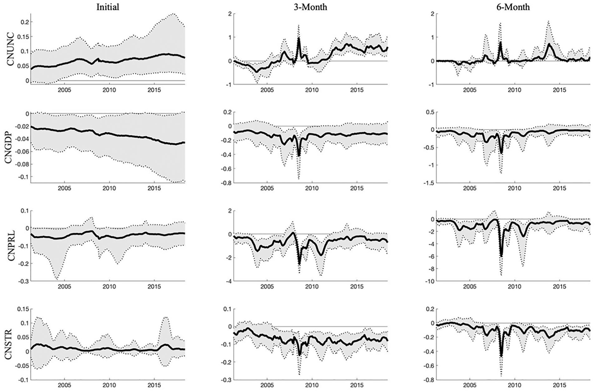
Time-varying (cumulative) responses of China’s macroeconomy to a 1% upsurge in U.S. economic uncertainty. The solid lines are the median posterior estimates of the IRFs, while the shaded regions are the 68% HPD intervals.

At first glance, there is compelling evidence of the time-varying effects of U.S. economic uncertainty shocks on Chinese economic activities. Interestingly, the IRFs are more volatile at horizons of 3 and 6-month after the shock than they are at the moment when the shock takes place. However, this result is not counter-intuitive. First, as our empirical study is based on a monthly frequency, it is unlikely that a rising shock in U.S. economic uncertainty would elicit an immediate and sizable impact on China’s macroeconomy since the spillovers of external shocks usually take time to be effective. Consequently, the initial IRFs displayed in Figure 4 are much smaller and relatively stable. As shown in Figure 3, U.S. economic uncertainty shocks take about 3 months to spill over to China, inducing remarkable reactions in Chinese economic activities. Second, as documented in Mumtaz and Theodoridis (2017) and Liu et al. (2020), institutional and policy changes, as well as the unstable global economy, are crucial factors that cause the responses of the domestic macroeconomy to external shocks to evolve over time. Thus, the IRFs at horizons of 3 and 6-month after the shock depend on different conditions at different times, resulting in high volatilities. Accordingly, we scrutinize the rationale behind the time-varying IRFs in the following section.

As shown in the top panel of Figure 4, a rise in U.S. economic uncertainty causes an instant increase in China’s economic uncertainty throughout the sample period. Moreover, this instantaneous response is relatively stable, increasing in magnitude over time and becoming significant from 2003 onward. However, the lagged responses in 3-month and 6-month after the shock are extraordinarily volatile: the estimated responses fluctuate dramatically and reach a peak during the period of global financial turmoil, which is roughly in line with Yin and Han (2014) and Liow et al. (2018). Furthermore, the responses hit another peak around 2014, when global economic activity was subdued, causing a great crash in the oil prices. Therefore, our results support the findings by IMF (2013) that the spillovers among uncertainties are more intense when common shocks emerge. In addition, the significance and sign of the responses also shift a lot during our sample period. Before 2005, China’s economic uncertainty is less responsive to U.S. economic uncertainty shocks in general and shown a mildly negative response in about 3 months after the shock around 2003. Nonetheless, the responses revert to be positive after 2005. Furthermore, China’s economic uncertainty tends to respond weakly from 2009 to 2010, which can be explained by the policies adopted by the Chinese government to protect its domestic economy from the impact of the global financial crisis, when the Chinese authorities had pegged its currency to the U.S. dollar again and implemented an economic stimulus plan. Since 2012, the responsiveness has been increasing on account of the accelerated pace of opening-up. However, the responses after 2015 are not as persistent as during the period when common shocks were encountered, fading away in about 6 months after the shock.

As the second panel of Figure 4 shows, U.S. economic uncertainty always imposes a negative shock to Chinese GDP. However, while the corresponding HPD interval, by and large, suggests a hike in U.S. economic uncertainty can only temporarily reduce China’s real GDP throughout our sample period, it has a strong and prolonged adverse impact on China’s GDP during the financial crisis. Interestingly, the impact of U.S. economic uncertainty on China’s GDP is small during tranquil times, which is counter-intuitive that the Chinese economy is highly interconnected with the United States in both trade and finance. One possible explanation is that the transmission mechanism of spillovers was mitigated. Although the United States has been China’s largest trading partner, the dependence of China’s GDP on bilateral trade with the United States has declined substantially since 2005. In 2005, exports to the United States accounted for nearly 7% of China’s GDP. This share, however, was halved in 2018. Moreover, the main driver of China’s economic growth is domestic consumption rather than exports (Sun, 2009). Furthermore, the improved financial markets, as well as the unique economic and political systems, have enabled the Chinese government to withstand unfavorable external shocks. For instance, the increasingly flexible exchange rate regime after 2005, especially after 2012, could help China insulate the adverse impact of foreign markets. In contrast to other countries, China has many levers combining fiscal and monetary instruments to stimulate economic growth, mainly through state-led investment. A bold fiscal policy, known as “the four trillion economic stimulus package,” launched in late 2008, shielded China from falling into a “western-style recession” (Y. Wen & Wu, 2019). These findings strengthen the conclusion of IMF (2013) that the dampening impact on Chinese GDP of U.S. economic uncertainty shocks is merely immediate and transient during the tranquil period, while it is persistent and intense in times of crisis. In addition, our results partially confirm the conclusion of Huang et al. (2018).

Also, the overall effects on China’s price level are negative and prolonged, although the instantaneous responses are generally less precise. Moreover, as shown in the penultimate panel of Figure 4, the responses to U.S. uncertainty shocks fluctuate considerably, with a trough during the global financial crisis around 2008. Apparently, the 68% HPD interval after 2012 is quite wide to contain zero, indicating that China’s price level is somewhat sticky in the face of U.S. economic uncertainty shocks. This stickiness of price level during this period might be attributed to improving global demand due to the recovery from the crisis and, in particular, the destocking reforms in China. Since 2012, China has implemented several reforms to reduce excess production capacity, such as “the structural reform on the supply-side” and “a rural revitalization strategy,” stabilizing the domestic market and causing China’s price level to be less responsive to U.S. economic uncertainty shocks.

The last panel of Figure 4 shows that short-term interest falls gradually with a lag of two months following a rise in U.S. economic uncertainty. The time-varying reactions of the interest rate -collective speaking- are in harmony with the responses of GDP and price level. Specifically, the interest rate responds little and insignificantly when GDP and price level respond little, while it falls considerably and significantly when encountering large drops in GDP and price level, especially during the global financial crisis. As discussed above, this kind of time-variant property of the interest rate responses is related to the monetary policy rule and risk premium of the money market. Although the short-term interest rate we use is market-oriented, it is still vulnerable to the influence of the monetary authority. Under a stylized monetary policy rule, for example, the Taylor rule, we can expect a fall in interest rates when both GDP and price level decline. Moreover, the market-oriented interest rate also varies in light of the risk premium of loans, including inflation risk. Therefore, as the price level declines, so as the risk of inflation, the interest rate accordingly falls in response to a leap in U.S. economic uncertainty.

To sum up, we provide evidence of the time-varying effects of U.S. economic uncertainty on the Chinese macroeconomy, that is, the strong detrimental effects in times of the global financial crisis and the lesser impacts during the tranquil period. As mentioned in the introduction, capital flows might play a crucial part in spillovers of uncertainty. During a crisis, a rising shock to economic uncertainty originating from the advanced economies would worsen international investors’ balance sheets, increasing the value at risk, which in turn reduces the willingness of international risk-taking and retrenches capital flows to emerging market economies. In addition, more capital outflows may be promoted by the signaling effect. Using the IMF’s BOP data, Broner et al. (2013) highlight substantial capital outflows from China during the 2008 global financial crisis. As a result, the local economy would be inevitably worsened. Moreover, the hindering effects on domestic economic activities of U.S. economic uncertainty are escalated during the 2008 global financial crisis when the United States has witnessed material reductions in consumption, investment, and other economic indicators. During this period, a rising shock to U.S. economic uncertainty would further reduce demand for foreign commodities and provoke negative shocks for U.S. trading partners through the trade channel. In addition, the appreciation of the Renminbi against the U.S. dollar since July 2005 has exacerbated China’s woes. In these regards, the Chinese economy would undergo striking detrimental impacts of U.S. uncertainty in the global financial crisis.

However, China has many countermeasures to withstand unfavorable external shocks and also restore economic growth. China’s central bank is somehow aggressive in responding to economic shocks through traditional and creative monetary policy tools. Consequently, the aggressive fiscal policy adopted in late 2008 has prevented China from a prolonged recession, making China’s GDP less responsive to U.S. uncertainty shocks during the post-crisis era, as our findings revealed. Moreover, even in the presence of a rising shock originating from the U.S. uncertainty during the tranquil period, China could insulate domestic economic growth from being affected by aggressive macroeconomic policies. For example, China has implemented several policies, such as expanding inputs on “eco-civilization building” and “poverty elimination plan,” as well as “the structural reform on the supply-side” around 2015, in response to the overcapacity caused by the sensational contraction in global demand since the second half of 2014.

Robustness Checks

To check the robustness of the results obtained from the baseline model, we consider the following four alternative specifications; (1) Following Colombo (2013) and Ludvigson et al. (2019), China’s economic uncertainty is ordered last to purge the uncertainty indicator from contemporaneous movements of macroeconomic variables (denoted as “CNUNC last”). (2) Following Carriero et al. (2018b), the VAR lag length is set to 6(denoted as “Lag 6”). (3) Proxying uncertainty with the EPU index constructed by Baker et al. (2016) (denoted as “EPU proxy”). (4) Since U.S. economic uncertainty shocks might transmit through the global commodity market, a global commodity price (excluding gold) index is taken into the model. In addition, Chinese consumption and investment are also included to picture a more comprehensive macroeconomy (denoted by “Global”). The global commodity price index is sourced from FRED and seasonally adjusted with the X12 method, while data for Chinese consumption and investment are retrieved from Chang et al.’s (2016) database. All these data are taken the log-difference to ensure stationarity. Following Cheng (2017), we order the variables as (USUNC, COMMODITY, CNUNC, CNINV, CNCON, CNGDP, CNPRL, CNSTR), where COMMODITY, CNINV, and CNCON stand for global commodity price, China’s investment, and consumption, respectively.

Despite the different specifications of variables and lags, the estimation procedure for all these models is same as that for the baseline model. The auto-correlation functions of residuals and the inefficiency factors of the estimated parameters for each model are reported in Appendix Figure A1 and Figure A2, respectively. In addition, the responses of China’s macroeconomy to a rising shock in U.S. economic uncertainty predicted by these models are displayed in Figures 5 and 6.

Figure 5.

Time-averaged (cumulative) responses to a 1% shock to U.S. economic uncertainty, selected Chinese variables, the posterior median estimates (solid lines), and the 68% HPD intervals (shaded regions).

Figure 6.

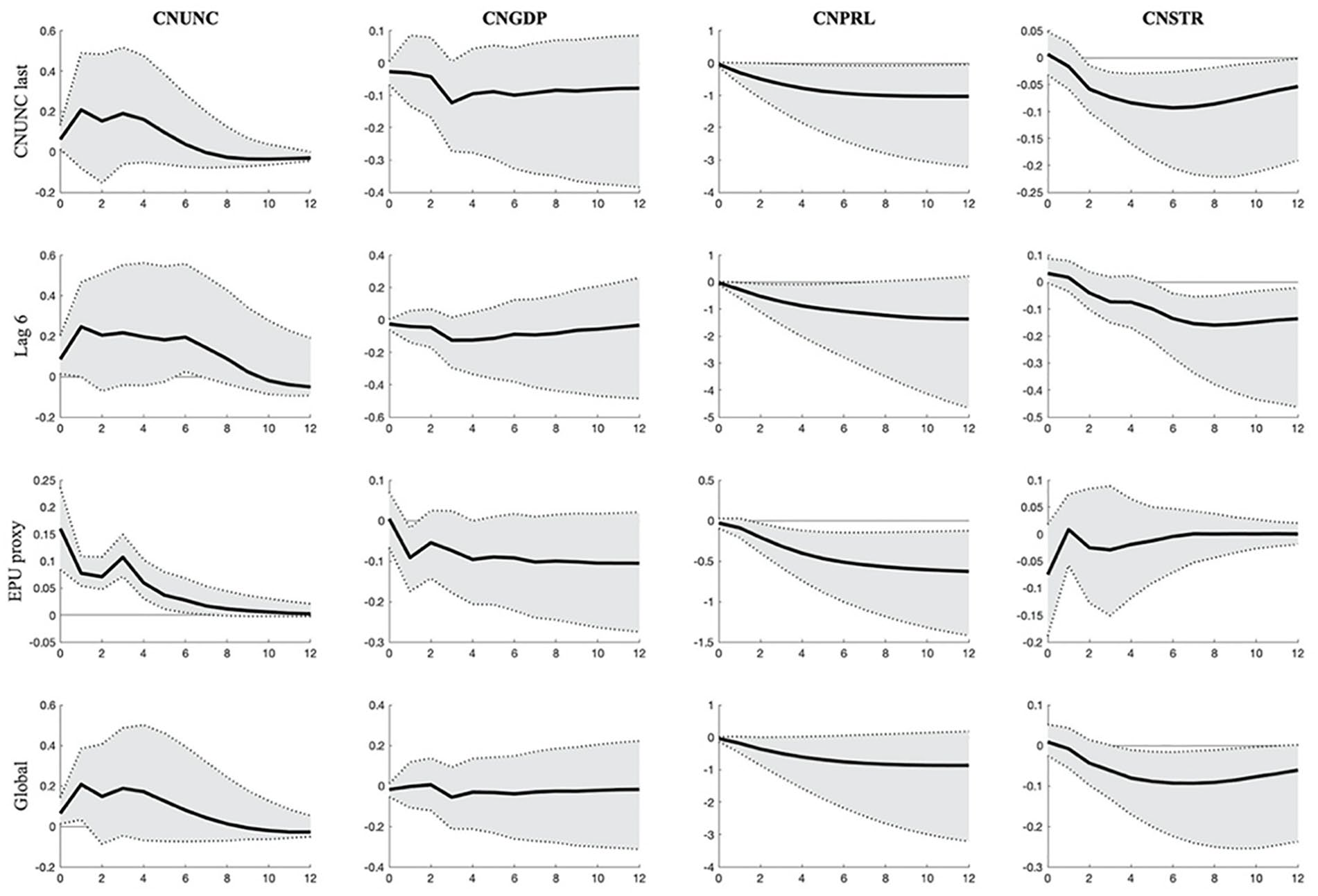
Time-varying (cumulative) responses of China’s macroeconomy at a horizon of 6 months after a 1% shock to U.S. economic uncertainty. The solid lines are the posterior median estimates, while the shaded regions represent the 68% HPD intervals.

As expected, the pattern that China’s macroeconomy responds to U.S. economic uncertainty shocks does not change with the ordering of China’s uncertainty, the VAR lag length, and the number of endogenous variables in the model. However, proxying uncertainty with EPU presents dramatically different results. More specifically, as shown in the penultimate panel of Figure 5, an increase in U.S. EPU triggers an immediate and more sizable rise in China’s EPU. However, after rebounding to a second peak 3 months after the shock, the response reverts and dwindles quickly. Moreover, the corresponding HDP interval indicates a more precise estimate. Further, the “EPU proxy” model predicts a significant negative response in China’s GDP in the first month after the shock, while a lesser but more significant response in China’s CPI. In addition, the interest rate responds insignificantly to the U.S. EPU shocks.

The difference between the “EPU proxy” model and the other models is more pronounced when inspecting the time-varying IRFs depicted in Figure 6. For brevity, we only report the IRFs at a horizon of 6 months after the shock. As we can see, the “EPU proxy” model produces more stable and significant responses in China’s economic uncertainty with a peak during the global financial crisis. However, the responses are less persistent in times of crisis, while are more persistent in tranquil period. Similar results are also found in the responses of China’s real GDP. In addition, the “EPU proxy” model significantly yields negative responses in China’s GDP before 2015. Nonetheless, the responses in China’s CPI are more persistent and significant under the “EPU proxy” model and have a trough during the financial crisis. Finally, and most differently, the response of the interest rate is extraordinarily time-dependent: it is negative and intense during the financial crisis but is significantly positive from 2011 to 2015, which conflicts with the economic theory.

More recently, Punzi (2020) argues that a rise in foreign uncertainty could cause domestic agents to postpone investment and reduce consumption, creating a negative shock to domestic growth. Under the “Global model,” we estimate the time-varying IRFs of China’s investment and consumption to a 1% shock to U.S. economic uncertainty and report the results in Figure 7. In contrast to Punzi (2020), we find that a rise in U.S. economic uncertainty would induce increases, with a peak during the global financial crisis, in China’s investment and consumption, resulting in little changes in real GDP (shown Figure 6). However, during the financial crisis, while China’s investment and consumption show positive responses to U.S. uncertainty shocks, the observed large and significant drop in GDP following a rise in U.S. uncertainty is inevitable because of the widespread and devastating effects of the crisis.

Figure 7.

Time-varying cumulative responses of China’s investment and consumption to a 1% shock to U.S. economic uncertainty. The solid lines are the posterior median estimates, while the shaded regions represent the 68% HPD intervals.

As a summary, our findings are robust to several model specifications but not to the specification of proxying EPU for economic uncertainty. However, all models signify a dramatically detrimental impact of U.S. economic uncertainty on China’s macroeconomy during the global financial crisis. The discrepancies among these models can be attributed to the inherent differences between the two measures of economic uncertainty. According to Jurado et al. (2015) and Baker et al. (2016), respectively, our estimated economic uncertainty meters the difficulty of predicting the macroeconomy, while EPU basically reflects the public media’s attention on the macroeconomy and especially economic policies. Consequentially, news reports concerning the economic outcomes prevail when local or international events erupt, boosting a higher EPU. As a result, EPU is not only an index measuring local uncertainty but is also more relevant to the uncertainty caused by international affairs (Shin et al., 2018), partly mirroring media sentiment. Given this property, a high degree of synchronization among EPU indices across countries can be expected, especially during the outbreak of international events. Therefore, the estimated spillovers of economic uncertainty might be biased if EPU is used as a proxy for economic uncertainty.

Conclusion

We assess the spillovers of U.S. economic uncertainty shocks on the Chinese macroeconomy from a time-varying perspective. Our empirical findings suggest that the detrimental impacts of U.S. economic uncertainty shocks on Chinese key macroeconomic variables evolve noticeably over time. Broadly speaking, U.S. economic uncertainty has sizable, durable, and significant effects during the global financial crisis, but small and transient effects in the tranquil times. Specifically, a rising shock to U.S. economic uncertainty leads to a persistent increase in China’s uncertainty and large drops both in GDP, price level, and short-term interest rate during the crisis in 2008, whereas a temporary increase in China’s uncertainty, an insignificant slight reduction in GDP, and small declines in price level and interest rate in other times of our sample period. Furthermore, our findings are robust to the ordering of China’s uncertainty, the VAR lag length, and the inclusion of more endogenous variables. However, the model using EPU to proxy uncertainty predicts similar but more stable responses in variables except the interest rate, which contradicts the economic theory, indicating EPU may not be a good indicator of local economic uncertainty.

The recent COVID-19 pandemic has paralyzed and has been reshaping the global economy. As two of the world’s leading countries, China and the United States have been extensively affected by the pandemic. Their economic activities have contracted dramatically due to containment measures to combat the virus but have rebounded strongly spurred by easing monetary policy and expanding fiscal expenditure since the second quarter of 2020. In particular, China’s remarkable recovery has attracted global attention, while the U.S. stock market rallied sharply, creating new levels continuously from November 2020 onwards. However, while China has successfully contained the pandemic, it is still raging in the United States, posing a substantial challenge to the U.S. economy. Thus, the newly elected Biden administration is expected to fight the pandemic scientifically and restore the U.S. economy, as well as normalize the U.S.-China relations. In contrast, the success in fighting against the pandemic ensures China have more fuel for stimulating economic growth. Notably, against a plummet in global demand due to the pandemic, the Chinese government recently has made several policies aiming at steering the economy primarily toward the domestic market (the so-called “domestic circulation”) and seeking a more diversified opening-up. Consistent with the IMF (2020), China was the only economy worldwide to sustain growth in 2020.

Importantly, our results have some policy implications. First, the opening-up is a double-edged sword that can foster rapid growth in many aspects and increase exposure to potential risks and uncertainties originating from other countries as well. Therefore, the strategy of opening-up should proceed with extreme caution. Second, when the globe faces a common shock, such as the global financial crisis and the recent COVID-19 pandemic, China should adopt more effective and potent policies to curb the detrimental effects caused by U.S. economic uncertainty shocks. Further, China should gradually reduce its dependence on the United States, seeking a more diversified and prudent pattern of opening-up. These can help China minimize the spillovers of U.S. economic uncertainty and enhance the independence of China’s macroeconomic policies, especially the monetary policy. Finally, investors holding Chinese assets are advised to be alert to the possible adverse effects on the fundamentals and to hedge or avoid the risk in advance.

In terms of research directions, further work could probe the factors shaping the spillovers of external uncertainty shocks on the domestic macroeconomy, as well as the countermeasures to mitigate the adverse concomitant spillovers. As we only focus on the macroeconomic level, another possible area of future study is the spillover effects on the microeconomic aspects, say, investor sentiment and investor myopia.

Footnotes

Appendix

Declaration of Conflicting Interests

The author(s) declared no potential conflicts of interest with respect to the research, authorship, and/or publication of this article.

Funding

The author(s) disclosed receipt of the following financial support for the research, authorship, and/or publication of this article: We gratefully acknowledge financial support from National Social Science Foundation of China under Grant 19BJY189.

ORCID iD

Lin Liu

References

Angelini

Bacchiocchi

Caggiano

Fanelli

(2019). Uncertainty across volatility regimes. Journal of Applied Econometrics, 34(3), 437–455. https://doi.org/10.1002/jae.2672

Angelini

Fanelli

(2019). Exogenous uncertainty and the identification of structural vector autoregressions with external instruments. Journal of Applied Econometrics, 34(6), 951–971. https://doi.org/10.1002/jae.2736

Antonakakis

Gabauer

Gupta

Plakandaras

(2018). Dynamic connectedness of uncertainty across developed economies: A time-varying approach. Economics Letters, 166, 63–75. https://doi.org/10.1016/j.econlet.2018.02.011

Baker

S. R.

Bloom

Davis

S. J.

(2016). Measuring economic policy uncertainty. The Quarterly Journal of Economics, 131(4), 1593–1636. https://doi.org/10.1093/qje/qjw024

Baumeister

Peersman

(2013). Time-varying effects of oil supply shocks on the US economy. American Economic Journal: Macroeconomics, 5(4), 1–28. https://doi.org/10.1257/mac.5.4.1

Benati

(2013). Economic policy uncertainty and the great recession [Working paper]. http://www.policyuncertainty.com/media/Uncertainty_Benati.pdf

Bloom

(2009). The impact of uncertainty shocks. Econometrica, 77(3), 623–685. https://doi.org/10.3982/ecta6248

Bloom

(2014). Fluctuations in uncertainty. Journal of Economic Perspectives, 28(2), 153–176. https://doi.org/10.1257/jep.28.2.153

Box

G. E. P.

Jenkins

G. M.

Reinsel

G. C.

Ljung

G. M.

(2015). Time series analysis: Forecasting and control. Wiley.

10.

Broner

Didier

Erce

Schmukler

S. L.

(2013). Gross capital flows: Dynamics and crises. Journal of Monetary Economics, 60(1), 113–133. https://doi.org/10.1016/j.jmoneco.2012.12.004

11.

Carriero

Clark

T. E.

Marcellino

(2018a). Endogenous uncertainty (Working Paper No. 18-05). Federal Reserve Bank of Cleveland. https://www.clevelandfed.org/newsroom-and-events/publications/working-papers/2018-working-papers/wp-1805-endogenous-uncertainty

12.

Carriero

Clark

T. E.

Marcellino

(2018b). Measuring uncertainty and its impact on the economy. The Review of Economics and Statistics, 100(5), 799–815. https://doi.org/10.1162/rest_a_00693

13.

Chan

J. C. C.

Eisenstat

(2018a). Bayesian model comparison for time-varying parameter VARs with stochastic volatility. Journal of Applied Econometrics, 33(4), 509–532. https://doi.org/10.1002/jae.2617

14.

Chan

J. C. C.

Eisenstat

(2018b). Comparing hybrid time-varying parameter VARs. Economics Letters, 171, 1–5. https://doi.org/10.1016/j.econlet.2018.06.031

15.

Chang

Chen

Waggoner

D. F.

Zha

(2016). Trends and cycles in China’s macroeconomy. NBER Macroeconomics Annual, 30, 1–84. https://doi.org/10.1086/685949

16.

Chang

Liu

Spiegel

M. M.

(2015). Capital controls and optimal Chinese monetary policy. Journal of Monetary Economics, 74, 1–15. https://doi.org/10.1016/j.jmoneco.2015.04.003

17.

Cheng

C. H. J.

(2017). Effects of foreign and domestic economic policy uncertainty shocks on South Korea. Journal of Asian Economics, 51, 1–11. https://doi.org/10.1016/j.asieco.2017.05.001

18.

Claeys

(2017). Uncertainty spillover and policy reactions. Ensayos sobre Política Económica, 35(82), 64–77. https://doi.org/10.1016/j.espe.2017.01.003

19.

Colombo

(2013). Economic policy uncertainty in the US: Does it matter for the Euro area? Economics Letters, 121(1), 39–42. https://doi.org/10/f5b5ht

20.

Davis

S. J.

Liu

Sheng

X. S.

(2019). Economic policy uncertainty in China since 1946: The view from mainland newspapers [Working paper]. https://stevenjdavis.com/s/EPU-in-China-View-from-Mainland-Newspapers-August-2019.pdf

21.

Eisenstat

Chan

J. C. C.

Strachan

R. W.

(2015). Stochastic model specification search for time-varying parameter VARs. Econometric Reviews, 35(8–10), 1638–1665. https://doi.org/10.1080/07474938.2015.1092808

22.

Fernald

J. G.

Spiegel

M. M.

Swanson

E. T.

(2014). Monetary policy effectiveness in China: Evidence from a FAVAR model. Journal of International Money and Finance, 49, 83–103. https://doi.org/10.1016/j.jimonfin.2014.05.007

23.

Gauvin

McLoughlin

Reinhardt

(2014). Policy uncertainty spillovers to emerging markets—Evidence from capital flows (Working Paper No. 512). Bank of England. https://www.bankofengland.co.uk/working-paper/2014/policy-uncertainty-spillovers-to-emerging-markets-evidence-from-capital-flows

24.

Geweke

(2005). Contemporary Bayesian econometrics and statistics. Wiley-Interscience.

25.

Granger

C. W. J.

(2008). Non-linear models: Where do we go next—Time varying parameter models? Studies in Nonlinear Dynamics & Econometrics, 12(3), Article 1. https://doi.org/10.2202/1558-3708.1639

26.

Gupta

Olasehinde-Williams

Wohar

M. E.

(2020). The impact of US uncertainty shocks on a panel of advanced and emerging market economies. The Journal of International Trade & Economic Development, 29(6), 711–721. https://doi.org/10.1080/09638199.2020.1720785

27.

Han

Yin

(2016). Macroeconomic policy uncertainty shocks on the Chinese economy: A GVAR analysis. Applied Economics, 48(51), 4907–4921. https://doi.org/10.1080/00036846.2016.1167828

28.

Huang

Tong

Qiu

Shen

(2018). The spillover of macroeconomic uncertainty between the U.S. and China. Economics Letters, 171, 123–127. https://doi.org/10.1016/j.econlet.2018.07.018

29.

Huber

Kastner

Feldkircher

(2019). Should I stay or should I go? A latent threshold approach to large-scale mixture innovation models. Journal of Applied Econometrics, 34(5), 621–640. https://doi.org/10.1002/jae.2680

30.

Iacoviello

Navarro

(2019). Foreign effects of higher U.S. interest rates. Journal of International Money and Finance, 95, 232–250. https://doi.org/10.1016/j.jimonfin.2018.06.012

31.

International Monetary Fund. (2013). World economic outlook.

32.

International Monetary Fund. (2020). World economic outlook: A long and difficult ascent.

33.

Jiang

Zhu

Tian

Nie

(2019). Determinants of within and cross-country economic policy uncertainty spillovers: Evidence from US and China. Finance Research Letters, 31, 195–206. https://doi.org/10.1016/j.frl.2019.08.004

34.

Jones

P. M.

Olson

(2015). The international effects of US uncertainty. International Journal of Finance & Economics, 20(3), 242–252. https://doi.org/10.1002/ijfe.1513

35.

Jurado

Ludvigson

S. C.

(2015). Measuring uncertainty. American Economic Review, 105(3), 1177–1216. https://doi.org/10.1257/aer.20131193

36.

Karnizova

(2014). Economic policy uncertainty, financial markets and probability of US recessions. Economics Letters, 125(2), 261–265. https://doi.org/10.1016/j.econlet.2014.09.018

37.

Kilian

Lütkepohl

(2017). Structural vector autoregressive analysis. Cambridge University Press.

38.

Klößner

Sekkel

(2014). International spillovers of policy uncertainty. Economics Letters, 124(3), 508–512. https://doi.org/10/f6kxn8

39.

Koop

(2003). Bayesian econometrics. Wiley-Interscience.

40.

Leduc

Liu

(2016). Uncertainty shocks are aggregate demand shocks. Journal of Monetary Economics, 82, 20–35. https://doi.org/10.1016/j.jmoneco.2016.07.002

41.

Liow

K. H.

Liao

W.-C.

Huang

(2018). Dynamics of international spillovers and interaction: Evidence from financial market stress and economic policy uncertainty. Economic Modelling, 68, 96–116. https://doi.org/10.1016/j.econmod.2017.06.012

42.

Liu

Zhang

M. M.

(2020). China’s economic policy uncertainty shocks and South Korea’s exports: A TVP-VAR approach with an SMSS structure. Journal of Korea Trade, 24(4), 1–17. https://doi.org/10.35611/jkt.2020.24.4.1

43.

Ludvigson

S. C.

(2019). Uncertainty and business cycles: Exogenous impulse or endogenous response? https://doi.org/10/ghmqh9

44.

Mumtaz

Theodoridis

(2017). The changing transmission of uncertainty shocks in the U.S. Journal of Business & Economic Statistics, 36(2), 239–252. https://doi.org/10.1080/07350015.2016.1147357

45.

Punzi

M. T.

(2020). The impact of uncertainty on the macro-financial linkage with international financial exposure. Journal of Economics and Business, 110, 105894. https://doi.org/10.1016/j.jeconbus.2020.105894

46.

Schmidt

Zwick

(2015). Uncertainty and episodes of extreme capital flows in the Euro area. Economic Modelling, 48, 343–356. https://doi.org/10.1016/j.econmod.2014.10.047

47.

Shin

Zhang

Zhong

Lee

D. J.

(2018). Measuring international uncertainty: The case of Korea. Economics Letters, 162, 22–26. https://doi.org/10.1016/j.econlet.2017.10.014

48.

Sun

(2009). China: Unscathed through the global financial tsunami. China & World Economy, 17(6), 24–42. https://doi.org/10.1111/j.1749-124X.2009.01172.x

49.

Trung

N. B.

(2018). The spillover effect of the US uncertainty on emerging economies: A panel VAR approach. Applied Economics Letters, 26(3), 210–216. https://doi.org/10.1080/13504851.2018.1458183

50.

Trung

N. B.

(2019). The spillover effects of US economic policy uncertainty on the global economy: A global VAR approach. The North American Journal of Economics and Finance, 48, 90–110. https://doi.org/10.1016/j.najef.2019.01.017

51.

Wen

Xiao

(2019). The effects of foreign uncertainty shocks on China’s macro-economy: Empirical evidence from a nonlinear ARDL model. Physica A: Statistical Mechanics and Its Applications, 532, 121879. https://doi.org/10.1016/j.physa.2019.121879

52.

Wen

(2019). Withstanding the great recession like China. The Manchester School, 87(2), 138–182. https://doi.org/10.1111/manc.12223

53.

World Bank. (2015). Global financial development report 2015/2016: Long-term finance.

54.

Yin

Han

(2014). Spillovers of macroeconomic uncertainty among major economies. Applied Economics Letters, 21(13), 938–944. https://doi.org/10.1080/13504851.2014.899665

U.S. Economic Uncertainty Shocks and China’s Economic Activities: A Time-Varying Perspective

Abstract

Keywords

Introduction

Related Literature

Methodology and Data

Empirical Model

Data

Proxies for economic uncertainty

Chinese macroeconomic variables

Empirical Results

Rationality of the Parameter Constancy Constraint

Results of the Baseline Model

Robustness Checks

Conclusion

Footnotes

Appendix

Declaration of Conflicting Interests

Funding

ORCID iD

References