Novel Optimization-Based Parameter Estimation Method for the Bass Diffusion Model

Abstract

The Bass model is the most popular model for forecasting the diffusion process of a new product. However, the controlling parameters in it are unknown in practice and need to be determined in advance. Currently, the estimation of the controlling parameters has been approached by various techniques. In this case, a novel optimization-based parameter estimation (OPE) method for the Bass model is proposed in the theoretical framework of system dynamics (SD). To do this, the SD model of the Bass differential equation is first established and then the corresponding optimization mathematical model is formulated by introducing the controlling parameters as design variable and the discrepancy of the adopter function to the reference value as objective function. Using the VENSIM software, the present SD optimization model is solved, and its effectiveness and accuracy are demonstrated by two examples: one involves the exact solution and another is related to the actual user diffusion problem from Chinese Mobile. The results show that the present OPE method can produce higher predicting accuracy of the controlling parameters than the nonlinear weighted least squares method and the genetic algorithms. Moreover, the reliability interval of the estimated parameters and the goodness of fitting of the optimal results are given as well to further demonstrate the accuracy of the present OPE method.

Keywords

Bass model parameter estimation system dynamics optimization

Introduction

Mathematical modeling of innovation diffusion developed by Bass in 1969 has received much attention of research community since the model can help them to better understand the market response to new products, assess new product introduction strategies, and make a model-based decision (F. M. Bass, 1969). The characteristic that distinguishes the Bass model from other growth models is that Bass explicitly incorporated some key behavioral assumptions from Rogers’ theory of diffusion of innovation (Rogers, 1962). Due to this, the Bass model has been widely applied in economic market to quantitatively forecast the new product sales (Fan et al., 2017; Moe & Fader, 2002), product life cycle (Guo, 2014), 3G mobile subscription in China (Lim et al., 2012), Diffusion of Mobile Telephony in China (Liu et al., 2012), oil production in the Eagle Ford Shale (Tunstall, 2015), marketing innovations to old-age consumers (Pannhorst & Dost, 2019), wind power development factors (She et al., 2019), and so on. More recently, the Bass diffusion model was extended to describe the consumer quantity of B2C commerce platforms (Li et al., 2020).

The classic Bass model includes three controlling parameters: the coefficient of innovation, the coefficient of imitation, and the total market potential. These parameters are practically unknown in advance and must be estimated based on some experimental or empirical data. This issue is the so-called parameter estimation problem. Therefore, the successful applications of the Bass model necessarily involve the determination of these parameters (Mahajan et al., 1991). Currently, the estimation of these parameters has been approached by many different techniques. For example, the ordinary least squares approach was first depicted by Bass for estimating the parameters in the diffusion model (F. M. Bass, 1969), and now it has become a very popular technique for parameter estimation (Dennis & Schnabel, 1996). Darija and Dragan estimated the parameters in the Bass model by the nonlinear weighted least squares (NLS) fitting approach, and the existence of the least squares estimate was theoretically proved (Marković & Jukić, 2013). Mahajan et al. (1986) developed a simple algebraic estimation procedure for the Bass diffusion model of new product acceptance. Yang and Wu established the Bass diffusion model of China Mobile user data by the NLS method and the genetic algorithms (AL) and reported that the AL was more suitable than the NLS approach for parameter estimation, especially when less data are available for building a growing product diffusion model (Yang & Wu, 2005). In addition, the maximum likelihood estimation approach for the Bass diffusion model was developed by Schmittlein and Mahajan to determine the new product acceptance (Schmittlein & Mahajan, 1982). Meng and He employed the ant colony algorithm (ACA) for parameter estimation in the Bass model and pointed out that the ACA performs better than the NLS and the AL (Meng & He, 2009). Satoh proposed a discrete Bass model featured by a difference equation and gave an ordinary least squares procedure for parameter estimation in this discrete Bass model (Satoh, 2001). However, the discrete Bass model can be applied only if a discrete equation with exact solution is derived. Recently, Grasman and Kornelis estimated the parameters of the Bass model using the numerical solution of the Bass equation, so discrete data of future sales can be obtained from the fitted model for the purpose of stock management (Grasman & Kornelis, 2019).

Although various techniques have been developed for parameter estimation in the Bass diffusion model, it is observed that these parameter estimation approaches may lead to different model fitting results that further affect the forecasting accuracy of the Bass model. So, how to improve the accuracy of model parameter estimation is still an open issue for ensuring the effectiveness and accuracy of the Bass diffusion model. In this study, an optimization-based parameter estimation (OPE) method for the Bass model is proposed based on the system dynamics (SD) theory. First, the mathematical description of the Bass model is translated into the SD model and its validity is assessed by the data check. Then, the OPE method of the Bass model is depicted by establishing the mathematical optimization model, which can be solved iteratively. Finally, the performance of OPE method is discussed by two examples.

SD Model of the Bass Model

Basic Form of Bass Model

To describe the time-dependent diffusion process of a new product, Bass proposed the following constant coefficient differential equation (F. M. Bass, 1969)

\frac{d y (t)}{d t} = p [m - y (t)] + \frac{q}{m} y (t) [m - y (t)],

(1)

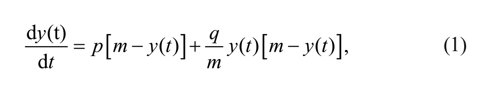
where $y (t)$ is the cumulative number of adopters (CNA) of a new product at time t, $p > 0$ is the coefficient of innovation, $q \geq 0$ is the coefficient of imitation, and $m > 0$ is the total market potential, that is, the maximum CNA to be reached.

Obviously, in Equation 1, the adoption rate term $d y (t) / d t$ is determined by the two additive terms: the term $p [m - y (t)]$ representing adoptions due to innovators and the term $\frac{q}{m} y (t) [m - y (t)]$ representing adoptions caused by imitators. Therefore, the function $y (t)$ and its derivative strongly depend on the coefficients $p$ , $q$ , and $m$ . Thus, we can rewrite the function $y (t)$ as

y = y (t, p, q, m) .

(2)

Typically, if the initial condition is assumed as $y (t = 0) = 0$ , the integration of Equation 1 can give the following analytical solution:

y (t, p, q, m) = m \frac{1 - e^{- (p + q) t}}{1 + \frac{q}{p} e^{- (p + q) t}}, t \geq 0,

(3)

and

\frac{d y (t, p, q, m)}{d t} = m \frac{{(p + q)}^{2}}{p} \frac{e^{- (p + q) t}}{{[1 + \frac{q}{p} e^{- (p + q) t}]}^{2}}, t \geq 0 .

(4)

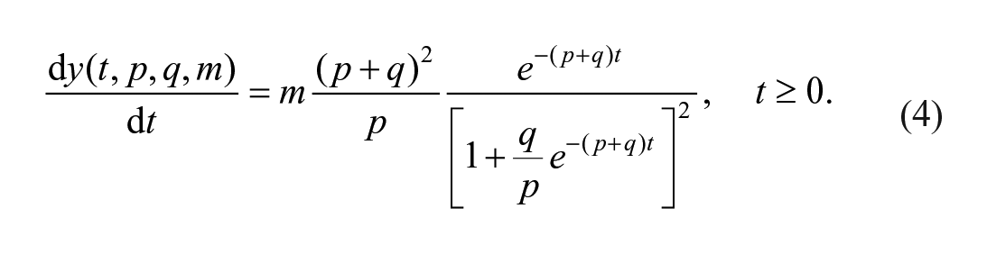
Moreover, from the analytical solution (3), it is derived that

\lim_{t \to \infty} y (t, p, q, m) = m .

(5)

Figure 1 clearly indicates the variations of the CNA function for various controlling parameters p and q under the assumption m = 1. It is found that all curves (almost) approach to the limit value m = 1. Moreover, the parameters p and q have a significant influence on the shape of the CNA curve. The higher the parameter p or q, the more easily the curve converges.

Figure 1.

Variations of the CNA function for various controlling parameters (m = 1).

Establishment of the SD Model

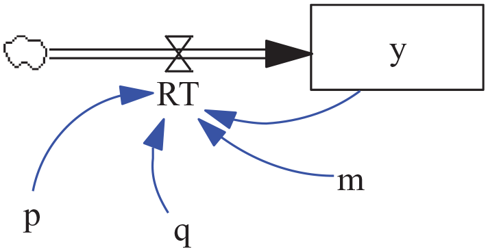
To establish the SD model corresponding to the Bass differential equation, a flow diagram is generally required from which the types of variables and the interrelation and connectivity between the variables can be clearly distinguished. Figure 2 is the flow diagram of the Bass model of interest by using the system dynamics software VENSIM, where the CNA function $y$ in Equation 1 is regarded as a state variable, the parameters $p$ , $q$ , and $m$ are exogenous variables, and RT is rate variable.

Figure 2.

Flow diagram of the Bass model.

According to the flow diagram, the SD model can be correspondingly established by translating the flow diagram into the SD equations. In other words, to establish the SD model, the relationship between different variables should be quantitatively described by the SD mathematical expressions. Because the differential equation of the Bass model is relatively simple, the SD expression to be defined is only the relationship between the rate variable and the exogenous variables, that is,

R T = p [m - y (t)] + q \frac{y (t)}{m} [m - y (t)] .

(6)

Generally, before running the SD simulation, the values of the parameters (p, q, m) of the Bass model must be assigned. However, these parameters are practically unknown in advance. In this study, they will be estimated by the optimization method to be developed subsequently.

Model Check

For the SD model, model checking is necessary to demonstrate the effectiveness of the model. However, there is no unique way for SD model testing (Barlas, 1989, 1996). J. W. Forrester, the founder of the SD theory, pointed out that the qualitative check method of the SD model is alternatively effective (Forrester & Senge, 1980). Here, the dimensional consistency check and time integral step check for the established SD model are carried out. Then a qualitative test is performed to meet the hypothesis of the Bass model defined as: the number of adopters $y$ increases when $p$ , $q$ , and $m$ increase, and vice versa.

The model qualitative testing shown in Figures 3 to 5 is performed under the initial assumption of $p = 0.1$ , $q = 0.1$ , and $m = 1000$ . In Figures 3 to 5, the red line refers to the curve evaluated by the initial parameters, and the blue line corresponds to the induced curve by the changed value of parameter. Figure 3 shows that when $p$ increases from 0.1 to 0.2, the function $y$ increases. Figure 4 shows that when $q$ increases from 0.1 to 0.35, the function $y$ increases as well. Figure 5 shows that when $m$ is reduced from 1,000 to 750, the function $y$ reduces too. Numerical experimental results show that the function of SD model is consistent with the hypothesis of the model.

Figure 3.

Variation of the function y with respect to the parameter p.

Figure 4.

Variation of the function y with respect to the parameter q.

Figure 5.

Variation of the function y with respect to the parameter m.

OPE Method

In general, according to a set of time-dependent reference data that include the values of CNA at different time instances, the values of model parameters p, q, and m can be estimated (F. M. Bass, 1969). In this study, the estimation of the parameters p, q, and m is conducted based on optimization operation of the SD model. To do this, the following optimization mathematical function is established

\begin{array}{l} {X} = {[p, q, m]}^{T} \\ \min F (X) = F_{o i} (X) - F_{r i} (i = 1, \cdot \cdot \cdot, n) \\ s . t . {X}_{d} \leq {X} \leq {X}_{u} \end{array},

(7)

where ${X}$ is the design variable array, whose elements are the parameters p, q, and m of the Bass model. $F (X)$ is the objective function consisting of $F_{o i} (X)$ and $F_{r i}$ . $F_{o i} (X)$ is the CNA function to be optimized. $F_{r i}$ is the reference function that $F_{o i} (X)$ is to be reached. n is the number of discrete time points

0 < t_{1} < t_{2} < \dots < t_{n},

(8)

at which the value of the CNA function $F_{o i} (X) = y (t_{i}, p, q, m)$ is to be determined, and the value of the reference function $F_{r i}$ is in some way obtained. ${X}_{l}$ and ${X}_{u}$ are the lower and upper limits of the design variables, respectively.

Besides, the solving of the optimization model needs an initial guess of the design variable, that is, ${X^{*}} = [p^{*}, q^{*}, m^{*}]$ .

The aim of this optimization model is to make the curve $F_{o i}$ to be optimized is as close as possible to the given reference curve $F_{r i}$ by optimizing the value of the design variable under the specific constraint. Because this procedure is related to mathematical optimizing theory, so it is called optimization-based parameter estimation (OPE) method. The OPE method can not only determine the estimated values of the parameters p, q, and m but also give the reliability and confidence interval of the estimated parameters.

Results and Analysis

Example 1

Reference data

To validate the accuracy of the OPE method for estimating the parameters p, q, and m of the Bass model, the reference function is obtained from the analytic solution (3) by assuming p = .001, q = 0.65, and m = 1,000 for convenience. It is worth noting that both $p$ and $q$ in the Bass model vary in the range of (0,1], and $p$ is always much less than $q$ (F. M. Bass, 1969). Moreover, the parameter $m$ representing the converged value of the CNA function (see Equation 5) is case-dependent and should be set according to the characteristic of problem of interest in practice. Here, $m = 1, 000$ is simply set without any special purpose. This set of reference data is listed in Table 1. Then, the OPE method is adopted to evaluate the optimal values of the parameters p, q, m, and the optimized CNA function. The validity of the OPE method can be demonstrated by comparing the optimized results to the analytical solutions.

Table 1.

Reference Data and Estimation Data.

Time (Day)	1	2	3	4	5	6	7	8
Exact CNA: y_i	1.41	4.10	9.21	18.87	36.87	69.60	126.50	218.20
CNA of OPE: ŷ_i	1.42	4.12	9.25	18.93	36.95	69.68	126.60	218.20
Time (Day)	9	10	11	12	13	14	15	16
Exact CNA: y_i	349.20	507.50	664.10	791.40	879.10	933.10	964.00	980.90
CNA of OPE: ŷ_i	349.10	507.40	664.10	791.40	879.30	933.20	963.90	980.80

Note. CNA = cumulative number of adopters; OPE = optimization-based parameter estimation.

Parameter estimation

To perform optimization, an initial guess of the design variable ( $[p^{*}, q^{*}, m^{*}] = [0.001, 0.5, 1000]$ ) is assumed, which significantly differs from the exact value, and the corresponding initial CNA curve is set as the initial curve of the function F_oi. The upper and lower limits of the design variables are defined as follows:

{[0.0001, 0.01, 10]}^{T} < {[p, q, m]}^{T} < {[1.0, 1.0, 1100]}^{T} .

(9)

With the SD optimization, the optimal values of the parameters p, q, and m by the OPE method are shown in Table 2 and the resulting CNA values are listed in Table 1. It can be seen from Tables 1 and 2 that the predicted results from the OPE method exhibit good convergence and high accuracy to the analytical solutions. Moreover, the OPE method also gives the parameter estimation interval under 95% reliability as shown in Equation 10,

\begin{array}{l} 0.0010049 \leq p = 0.0010094 \leq 0.0010140 \\ 0.64996 \leq q = 0.65041 \leq 0.65088 \\ 988.835 \leq m = 999.726 \leq 1000.610 . \end{array}

(10)

Table 2.

Accuracy of Parameter Estimates.

Parameter	p	q	m
Original value	0.001	0.650	1,000
Optimal value	0.0010094	0.65041	999.726
Error (%)	0.93	0.06	0.03

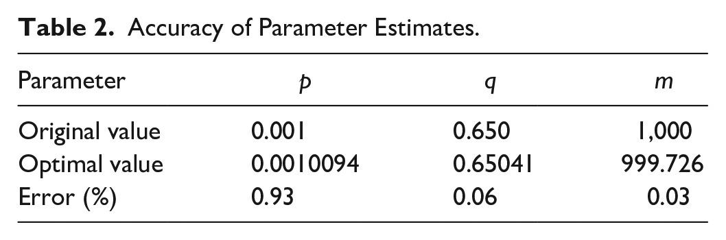
Figure 6 shows the curves y:aREF, y:aRR1, and y:aRR2 after the implementation of OPE method. The curve y:aREF is the reference CNA curve in which the data are the exact CNA y_i in Table 1. The curve y:aR1 is the initial curve corresponding to the initial guess of parameter p, q, and m. The curve y:aR2 is the optimized CNA curve obtained by the OPE method. It can be seen that the curves y:aRR2 and y:aRFRF show extremely good agreement.

Figure 6.

Variations of the initial, reference, and optimal curves in Example 1.

To measure the quality of the optimal results, the following goodness of fitting ( $R^{2}$ ) is defined:

R^{2} = 1 - \frac{\sum_{i = 1}^{n} {(y_{i} - {\hat{y}}_{i})}^{2}}{\sum_{i = 1}^{n} {(y_{i} - {\bar{y}}_{i})}^{2}},

(11)

where ${\hat{y}}_{i}$ and $y_{i}$ denote the estimated values and the reference values of the CNA function, respectively. ${\bar{y}}_{i}$ is the average of the reference values. Here, the reference value of $y_{i}$ is the exact value obtained from Equation 3, as listed in Table 1.

Using Equation 11, the goodness of fit of the optimal curve y:aRR2 is 0.9999. Therefore, it is confirmed that the minimization of the objective function $F$ defined by Equation 7 provides a much good fitness of the CNA function to the reference function.

Example 2

In the second example, the real case on the evolution of the number of users of China Mobile is taken into consideration, and the user diffusion model from China Mobile is solved to demonstrate the performance of the present OPE method.

China mobile user data

Yang and Wu calculated the number of 2G users per year (NUPY) of China Mobile from 1991 to 2004 by the statistics method (Yang & Wu, 2005), which are listed in Table 3 (unit: ten thousand). The change in NUPY was described by the Bass diffusion model, in which the values of the parameters p, q, and m were estimated by Yang and Wu using the NLS method and the genetic algorithm (AL), respectively (Yang & Wu, 2005). Here, the results from the NLS and AL methods will be compared to those from the present OPE method.

Table 3.

Real 2G User Data of China Mobile (Unit: Ten Thousand) (Yang & Wu, 2005).

Time	1991	1992	1993	1994	1995	1996	1997
NUPY:y_i	4.7	18.0	64.0	166.8	362.9	685.3	1,323.0
Time	1998	1999	2000	2001	2002	2003	2004
NUPY:y_i	2,386.0	4,330.0	8,453.0	14,522.0	20,661.0	26,863.0	33,482.0

Parameter estimation

To solve the SD optimization model defined in Equation 7, an initial guess of the design variable is assumed as $[p^{*}, q^{*}, m^{*}] = [0.0002, 0.65, 33, 482]$ , with which the initial curve of the function $F_{o i}$ to be optimized can be determined. Here, the initial value of the parameter $m$ is set as 33,482, the maximum value of NUPY in Table 3, because $m$ is case-dependent and represents the converged value of the NUPY in the Bass model. The real user data $y_{i}$ in Table 3 corresponds to the reference curve $F_{r i}$ . The upper and lower limits of the design variable are assumed as

0.0001 \leq \leq p \leq 1, 0.0001 \leq q \leq 1, 5 \leq m \leq 40, 000 .

(12)

0.0001 ≤ p ≤ 1, 0.0001 ≤ q ≤ 1, 5 ≤ m ≤ 40,000. (12)

Using the VENSIM software, the present SD optimization model is solved and the optimal values of the parameters p, q, and m are obtained as $p = 0.0002, q = 0.72466, m = 39, 485.7$ . Moreover, the estimation interval under 95% reliability of the parameters is given by

\begin{array}{l} 0.00019981 \leq p = 0.0002 \leq 0.00020077 \\ 0.72462 \leq q = 0.72466 \leq 0.72467 \\ 39, 842.9 \leq m = 39, 845.7 \leq 39, 847.2 . \end{array}

(13)

Figure 7 shows the variations of the initial curve y:bR1, the optimal curve y:bR2, and the reference curve y:bREF. It can be seen that the optimal results are in good agreement with the reference (real) results.

Figure 7.

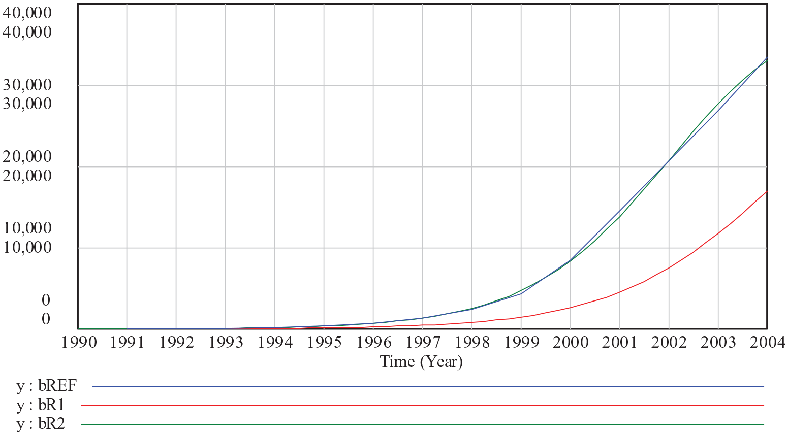
Variations of the initial, reference, and optimal curves in Example 2.

Comparison of parameter estimations

In this section, the estimated results from the NLS method, the AL method, and the present OPE method are compared to demonstrate the advantage of the present method. Table 4 lists the estimated results of the parameters p, q, and m. It is observed from Table 4 that the OPE and AL methods give similar level of the parameter estimates, which look more reasonable than that from the NLS method. To further illustrate the comparison, Table 5 lists the CNA results from the three estimation methods. It is indicated that the OPE method produces better predictions than the NLS and AL methods, especially after the year 1993. To show the variation of the predictions more clearly, the CNA results are plotted in Figure 8. It can be seen from Figure 8 that the curve estimated by the OPE method is closer to the actual data curve than that estimated by the NLS method and the AL method. Among the three methods, the NLS method performs worst.

Table 4.

Estimated Parameter Values From the Three Different Methods.

Parameter	p	q	m
OPE	0.0002	0.7247	39,486
NLS	0.0003	0.6940	28,884
AL	0.0001	0.7552	33,450

Note. AL = genetic algorithm; NLS = nonlinear weighted least squares; OPE = optimization-based parameter estimation.

Table 5.

Comparison of User Data of China Mobile (Unit: Ten Thousand).

Time	Actual data	OPE	NLS	AL
1991	4.7	14.3	2.2	7.1
1992	18.0	38.2	7.5	22.2
1993	64.0	84.7	20.4	54.2
1994	166.8	175.0	51.7	122.5
1995	362.9	349.7	127.1	266.5
1996	685.3	686.2	308.6	569.5
1997	1,323.0	1,328.0	740.2	1,197.5
1998	2,386.0	2,526.0	1,739.9	2,460.5
1999	4,330.0	4,685.0	1,956.2	4,855.5
2000	8,453.0	8,325.0	6,045.2	8,921.5
2001	14,522.0	13,800.0	12,057.2	14,665.5
2002	20,661.0	20,730.0	18,228.2	20,953.5
2003	26,863.0	27,660.0	22,611.2	26,168.5
2004	33,482.0	33,050.0	25,849.2	29,595.5

Note. AL = genetic algorithm; NLS = nonlinear weighted least squares; OPE = optimization-based parameter estimation.

Figure 8.

Curves of actual data and estimation data of user.

On the contrary, the mean values of the predicted user data from the three methods and their goodness of fitting (R²) to the actual data are listed in Table 6. The average value of the actual data is 8,094.4. It is found from Table 6 that the average value from the OPE method is the closest to the average value of the actual data than that from the other two methods. The relative error between the OPE prediction and the actual value is 0.14% only. Correspondingly, the OPE method gives the best R² value, as expected.

Table 6.

Comparison of Fitting Degree of Curves of Three Estimation Methods.

Method	OPE	NLS	AL
Mean value	8,105.5	6,410.3	7,847.1
R ²	0.999	0.939	0.990

Note. AL = genetic algorithm; NLS = nonlinear weighted least squares; OPE = optimization-based parameter estimation.

To further illustrate the effectiveness of the present OPE method, the number of 4G user data per half year (NUPHY) of Chinese Mobile issued by Ministry of Industry and Information Technology of the People’s Republic of China in 2019 is analyzed. The 4G user data from December 2014 to December 2018 are tabulated in Table 7. For convenience of plotting, the time record is numbered with digit.

Table 7.

4G Mobile Phone User Data in China (Unit: Ten Thousand).

Time	2014/12	2015/06	2015/12	2016/06	2016/12
Number	1	2	3	4	5
NUPHY:y_i	11,787	22,546	38,622	58,458	76,994
Time	2017/06	2017/12	2018/06	2018/12
Number	6	7	8	9
NUPHY:y_i	88,812	99,688	110,950	116,546

Note. NUPHY = the number of 4G user data per half year.

To solve the SD optimization model defined in Equation 7, the initial guess of the design variable is assumed as [p*, q*, m*] = [0.05, 0.8, 140,000], with which the initial curve of the function F_oi to be optimized can be plotted. The real user data in Table 7 corresponds to the reference curve F_ri. The upper and lower limits of the design variable [p, q, m] are assumed as

0.0001 \leq p \leq 1, 0.0001 \leq q \leq 1, 3 \leq m \leq 150, 000 .

(14)

0.0001 ≤ p ≤ 1, 0.0001 ≤ q ≤ 1, 3 ≤ m ≤ 150,000. (14)

The SD optimization model of this problem is solved using the VENSIM software, and the optimal values of the parameters p, q, and m are obtained as Equation 15. The estimation interval with 95% reliability of the parameters is given by

\begin{array}{l} 0.0728966 \leq p = 0.0728978 \leq 0.0729465 \\ 0.405233 \leq q = 0.405236 \leq 0.405239 \\ 126, 070 \leq m = 126, 072 \leq 126, 079 . \end{array}

(15)

Figure 9 shows the variations of the initial curve y:cR1, the optimal curve y:cR2, and the reference curve y:cREF. It can be seen from Figure 9 that the optimal curve is in good agreement with the reference curve representing the real user data. Moreover, the R² of the results of the optimal curve y:cR2 to the real data is calculated according to Equation 11, and the value is R² = .9986.

Figure 9.

Variations of the initial, reference, and optimal curves for 4G user analysis in Example 2.

Finally, it can be seen from the solving procedure previously that the implementation of the SD-based OPE method is fully independent of the exact solution of the problem. The algorithm can be implemented as long as the corresponding SD model can be established. This means that the present OPE method can be extended for solving more complex Bass-type problems including more controlling parameters.

Conclusion and Future Work

Summary

Although the Bass model is attractive due to its conciseness and effectiveness, parameter estimation is still a critical issue for the application of the Bass model because the three parameters in the Bass model are unknown in advance in the practice. In this case, the novel OPE method is proposed for estimating the three controlling parameters and the variation of CNA function of the Bass model. To do this, the Bass differential equation is first translated into the SD expression representing the relationship between the rate variable and the exogenous variables, and then the SD-based optimization model is established by introducing the design variable, the objective function, and the constraint condition of the design variable. Subsequently, the present SD-based optimization model is solved by the VENSIM software, and its effectiveness and accuracy are demonstrated by the two case studies. The main conclusions of this work include the following:

To the best knowledge of the author, the present OPE method is the first attempt for solving the Bass model in the framework of system dynamics.

The present OPE model involves the SD equations of the problem which can be easily implemented.

The present OPE method exhibits excellent performance in parameter estimation and function prediction, and the accuracy is better than that of the NLS and AL methods.

The present OPE method provides an excellent model analysis technique and can be extended to more Bass-type problems such as forecasting mortality caused by COVID-19 (Gurumurthy & Mukherjee, 2020) and exploring the needs and experiences of educators (J. Bass et al., 2020).

Future Research

The case shows how the novel SD-based optimization model can be used to solve the Bass model of product diffusion, including the parameter estimation and the optimal prediction of CAN function. However, this work has several limitations that should be addressed in future research. First, we have only studied the three-parameter Bass model; however, the more complex diffusion model, that is, food safety information diffusion (Liang, 2021), including more controlling parameters, may be encountered. The related methodological process should be developed following the idea in this study. Second, in addition to the Bass model, the diffusion models available also include Logistic model and Gompertz model. These models may differ with the different study period (Liu et al., 2012). Therefore, further forecasting performance assessment of these diffusion models and the related optimal models are interesting for future research.

Footnotes

Declaration of Conflicting Interests

The author(s) declared no potential conflicts of interest with respect to the research, authorship, and/or publication of this article.

Funding

The author(s) disclosed receipt of the following financial support for the research, authorship, and/or publication of this article: The research is partially supported by the Science and Technology Development of Henan Province (No: 142102210563).

ORCID iD

Lang Liang

Ethics Statement

The author stated that no animal and human studies were included in this work.

References

Barlas

(1989). Multiple tests for validation of system dynamics type of simulation models. European Journal of Operational Research, 42(1), 59–87.

Barlas

(1996). Formal aspects of model validity and validation in system dynamics. System Dynamics Review, 12(3), 183–210.

Bass

F. M.

(1969). A new product growth for model consumer durables. Management Science, 15(5), 215–227.

Bass

Sidebotham

Creedy

Sweet

(2020). Exploring the needs and experiences of educators in facilitating use of the Bass model of holistic reflection. Nurse Education in Practice, 46, Article 102805.

Dennis

J. E.

Schnabel

R. B.

(1996). Numerical methods for unconstrained optimization and nonlinear equations. SIAM.

Fan

Z. P.

Che

Y. J.

Chen

Z. Y.

(2017). Product sales forecasting using online reviews and historical sales data: A method combining the Bass model and sentiment analysis. Journal of Business Research, 74, 90–100.

Forrester

J. W.

Senge

P. M.

(1980). Test for building confidence in System Dynamics models. In Legasto Jr

A. A.

Forrester

J. W.

Lyneis

J. M.

(Eds.), TIMS Studies in the Management Sciences (pp. 209–228). North-Holland Publishing Company.

Grasman

Kornelis

(2019). Forecasting product sales with a stochastic Bass model. Journal of Mathematics in Industry, 9(1), Article 2.

Guo

(2014). A novel Bass-type model for product life cycle quantification using aggregate market data. International Journal of Production Economics, 158, 208–216.

10.

Gurumurthy

Mukherjee

(2020). The Bass Model: A parsimonious and accurate approach to forecasting mortality caused by COVID-19. International Journal of Pharmaceutical and Healthcare Marketing, 14(3), 349–360.

11.

Yuan

Shi

Wang

Chan

F. T. S.

Ruan

(2020). An extended Bass Model on consumer quantity of B2C commerce platforms. Electronic Commerce Research, 20(3), 609–628.

12.

Liang

(2021). A study of system dynamics modelling and optimization for food safety risk communication in China. Alexandria Engineering Journal, 60(1), 1917–1927.

13.

Lim

Nam

Kim

Rhee

Lee

(2012). Forecasting 3G mobile subscription in China: A study based on stochastic frontier analysis and a Bass diffusion model. Telecommunications Policy, 36(10), 858–871.

14.

Liu

Chu

(2012). Diffusion of mobile telephony in China: Drivers and forecasts. IEEE Transactions on Engineering Management, 59(2), 299–309.

15.

Mahajan

Muller

Bass

F. M.

(1991). New product diffusion models in marketing: A review and directions for research. In Nakićenović

Grübler

(Eds.), Diffusion of technologies and social behavior (pp. 125–177). Springer.

16.

Mahajan

Sharma

(1986). A simple algebraic estimation procedure for innovation diffusion models of new product acceptance. Technological Forecasting and Social Change, 30(4), 331–345.

17.

Marković

Jukić

(2013). On parameter estimation in the bass model by nonlinear least squares fitting the adoption curve. International Journal of Applied Mathematics and Computer Science, 23(1), 145–155.

18.

Meng

F. D.

M. S.

(2009). Comparison and research of several parameter estimation approaches of Bass model (in Chinese). Computer Simulation, 26(1), 296–300.

19.

Moe

W. W.

Fader

P. S.

(2002). Using advanced purchase orders to forecast new product sales. Management Science, 21(3), 347–364.

20.

Pannhorst

Dost

(2019). Marketing innovations to old-age consumers: A dynamic Bass model for different life stages. Technological Forecasting and Social Change, 140, 315–327.

21.

Rogers

E. M.

(1962). Diffusion of innovations. The Free Press.

22.

Satoh

(2001). A discrete Bass model and its parameter estimation. Journal of the Operations Research, 44(1), 1–18.

23.

Schmittlein

D. C.

Mahajan

(1982). Maximum likelihood estimation for an innovation diffusion model of new product acceptance. Marketing Science, 1(1), 57–78.

24.

She

Z. Y.

Cao

Xie

B. C.

J. J.

Lan

(2019). An analysis of the wind power development factors by Generalized Bass Model: A case study of China’s eight bases. Journal of Cleaner Production, 231, 1503–1514.

25.

Tunstall

(2015). Iterative Bass Model forecasts for unconventional oil production in the Eagle Ford Shale. Energy, 93, 580–588.

26.

Yang

J. H.

C. Y.

(2005). To compare two kinds of estimates on the parameters of Bass Model (in Chinese). The Journal of Quantitative & Technical Economics, 12, 125–132.