Sage Journals: Discover world-class research

Abstract

When a firm has a target capital structure, it is usually in a book-value term rather than a market-value one as normally assumed in standard finance textbooks. This article provides a systematic approach to determine the optimal book-value debt ratio. The proposed method balances both the tax benefit of debt and its associated bankruptcy cost and more importantly incorporates the aims to maintain a good credit rating, financial robustness in times of adverse shocks, and financial flexibility to seize good investment opportunities. In terms of methodology, our model incorporates the tax benefit of debt in the form of lower cost of capital, whereas the expected bankruptcy cost is reflected in a higher credit spread. We adjust the Hamada equation to take default risk into account by applying the method suggested by Cohen when adjusting the cost of equity as a debt ratio changes. The model is calibrated to data from the U.S. non-financial firms. It provides predictions concerning the effects of key variables such as profitability and growth. Our model reveals a negative relationship between growth opportunities and market debt ratios but no clear directional relationship with book debt ratios. In addition, our model points to the negative (positive) relationship between profitability and market (book) debt ratio. Interestingly, the two debt ratios move in the opposite directions. These predictions have support from existing empirical literature.

Keywords

capital structure cost of capital debt ratio leverage ratio credit rating

Introduction

When a firm decides the mix of debt and equity to finance its investment, it wants a mix of a capital structure that maximizes its value. Debt provides benefits in the form of tax-saving and managerial discipline. However, it also increases financial distress costs, including bankruptcy costs, and costs of investor conflicts. A firm must balance the pros and cons to minimize its cost of capital or weighted average cost of capital (WACC) as explained in the standard trade-off theory (Kraus & Litzenberger, 1973). Finance theories suggest that a firm should consider the optimal debt ratio only in terms of market values.

Empirically, however, Welch (2004) find that U.S. firms do not counteract the mechanistic effects of changes in their stock prices on their market-value debt-equity ratios. To maintain their optimal ratios, firms are supposed to issue more (less) debts, repurchase more (less) shares, pay higher (lower) dividends, or issue less (more) new shares when their stock prices increase (decrease), but mostly they do not. Consequently, their market debt-equity ratios vary closely with fluctuations in their stock prices.

When a firm has a target capital structure, it is usually in book-value terms rather than market-value terms as presumed by capital structure theories (Fernandez, 2007). The reason as pointed out by Fernandez (2007) is that it is a book-value debt ratio that creditors and rating agencies pay attention to and put in their loan contracts.

The difference in focus on market-value debt ratios in capital structure theories and on book-value debt ratios among practitioners motivates this study. The current method based mostly on the trade-off model is to search for the optimal market debt ratio (Damodaran, 2012). There is no practical way to search for the optimal book debt ratio as the valuation models are based solely on the market debt ratios as pointed out by Fernandez (2007).

This article proposes a novel systematic approach to determine the optimal book-value debt ratio. Our model incorporates the tax benefit of debt in the form of lower cost of capital, whereas the expected bankruptcy cost is reflected in a higher credit spread. This article improves over the conventional de-leveraging or re-leveraging method using the Hamada equation (Hamada, 1972) by incorporating default risk as proposed by Cohen (2004, 2007).

In addition, this article specifically applies the Fernandez (2007) valuation model which assumes that a firm targets its capital structure in a book-value term rather than a market-value one as normally presumed in other valuation models. We introduce formal measures of financial robustness and financial flexibility based on the idea of Koller et al. (2015). We then reveal the inherent trade-off between these qualities and the potential tax-saving benefit of debt.

Our model focuses on the case of a constant perpetual growth. The additional case of a constant level of debt with no growth similar to the original MM formula (Modigliani & Miller, 1958) is reported as an extension in Supplemental Appendix A-10. We then compare calibrated numerical predictions from our model to the actual observed data of the average U.S. non-financial firms.

In terms of key findings, our results show that within a certain range, a tax rate has a minimal impact on leverage, but it would have a huge impact when it crosses certain thresholds. With respect to the relationship between growth opportunities and book debt ratios, our results reveal an almost no directional relationship. With respect to the relationship between profitability and debt ratios, our results reveal that the market (book) debt ratio has a negative (positive) relationship with profitability.

In terms of contributions, first, our results illustrate the importance of credit rating as a firm attempts to maximize a tax-saving benefit from debt and maintains its optimal credit rating. Second, this article shows theoretically why most studies (e.g., Jong et al., 2008) fail to find significant tax effects on leverage. The traditional explanation is that the debt-to-equity ratios are simply cumulative results of separate decisions. There is no theoretical explanation. In this work, we show that a higher tax rate would lead to higher optimal both market and book debt ratios. However, the relationships are not linear but stepwise.

Third, this article explain theoretical reasons why growth has ambiguous effect on book debt ratio as found in the existing literature (e.g., Fama and French, 2002; Gul, 1999). Basically, we argue that the effect of an increase in a perpetual growth rate on the book debt ratio is the net effect of two opposing forces. The first one is a higher firm value, which results in more borrowing given the same market debt ratio. The second one is a lower optimal market debt ratio. This leads to a lower book debt ratio given the value of the firm. These two opposing forces cancel each other mostly, but over certain ranges, the second one dominates. That is when we see the negative relationship between growth opportunities and book debt ratios as found in the studies by Rajan and Zingales (1995), Jong et al. (2008) and Antoniou et al. (2008).

Fourth, our model also reveals that generally there are no clear directional relationship between growth opportunities and book debt ratios, whereas the traditional trade-off theory itself does not give a clear prediction concerning this relationship (Fama & French, 2002; Xu, 2012). The reason is that higher profitability would not only lead to a lower optimal market debt ratio as predicted by the trade-off, pecking order, and other theories, but also a higher firm value. These two opposing forces would mostly cancel each other effects.

Finally, we derive theoretical relationships between the risk-free rate, and debt ratios (both market and book) based on the trade-off model framework. Our model reveals that the market debt ratios would increase gradually with a periodic jump. In contrast, the book debt ratios would generally decrease due to the lower value of the firm from a higher cost of capital. However, it will rise periodically when a firm decides to increase its market debt ratios.

In terms of practical implications, this article provides a method for a firm to approximate its optimal book debt ratios. The method could be applied even in the case of non-listed firms. It also provides a formal framework to consider a trade-off between a higher tax-saving benefit from more debt and a lower financial flexibility and robustness from such debt.

To save space, literature reviews and detailed derivations are all in the Supplemental Appendix.

Optimal Capital Structure in a Case of a Constant Book-Value Debt Ratio With a Constant Growth

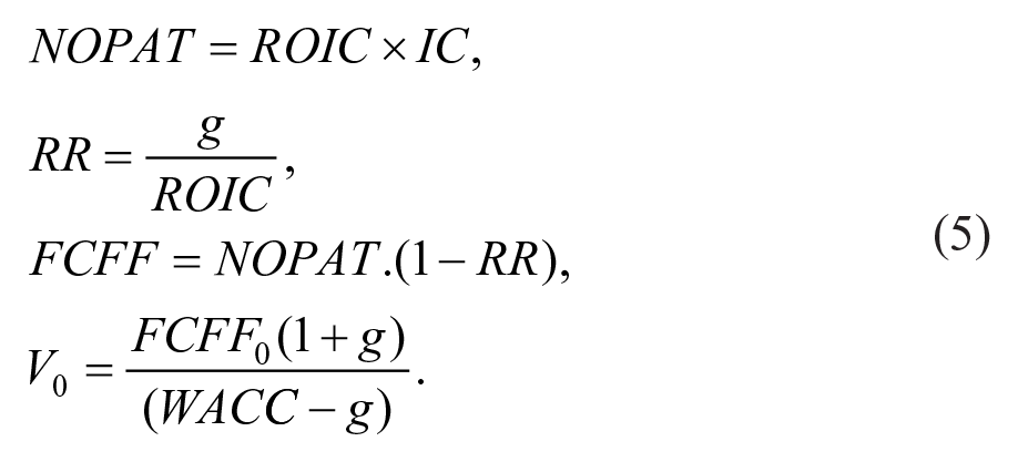
This article follows Fernandez (2007) in terms of determining the optimal capital structure in terms of a book-value debt ratio. In this case, we focus on a steady state of a constant growth. We assume a constant return on invested capital (ROIC). “ROIC” is simply net operating profit after tax (NOPAT) (a profit that a firm would have had if it has no debt) divided by invested capitals (ICs) or operating assets. We combine this with another assumption of a constant reinvestment rate (RR) which is defined as net capital expenditure (Net Capex) over NOPAT. Since a reinvestment is required to maintain a constant growth, the free cash flow to firm (FCFF) will equal to NOPAT times 1 minus RR.

We assume that shareholders would get nothing back in return when the company defaults on its debt and a default happens when a firm’s value is lower than the book-value of debt. In addition, existing debt would be repriced immediately to reflect a higher cost when a firm increases its leverage and its credit rating starts to deteriorate. As such, the book-value of debt and the market-value of debt would be the same.

Theoretical Model

Fernandez (2007) shows that if a firm maintains its book-value debt-to-equity ratio (B/DE) and a firm has a constant growth, then the value of debt tax shield will be a summation of a constant debt tax shield and a present value of tax-saving from an expected growth in future debt. The values of debt tax shield (VTS) and levered beta are determined in the following equations:

\begin{array}{l} V T S = (\frac{r_{u}}{r_{u} - g}) . T . D, \\ β_{l} = [1 + (1 - T) . (\frac{D}{E})] . β_{u}, \end{array}

(1)

where, β_l and β_u are the levered and unlevered betas, respectively. D/E is the market-value debt-to-equity ratio, and T is the corporate income tax rate. Derivations of the value of debt tax shield and levered beta in the case of a constant book-value ratio are reported in Supplemental Appendices A-6 and A-7, respectively.

Note that even though the value of tax shield in this case, r_u/(r_u – g).T.D, is higher than the one in the case of a constant level of debt (T.D), the values of levered beta are still determined by the same equation (see Supplemental Appendix A-10 for the case of a constant level of debt with zero growth).

After we plug this levered beta equation into the capital asset pricing model (CAPM) and the WACC formula, we will get the following equations (see Supplemental Appendix A-7), where W_d is the market-value debt ratio defined as the market-value of debt over the firm value.

\begin{array}{l} r_{e} = r_{u} + (1 - T) . (\frac{D}{E}) . (r_{u} - r_{f}), \\ W A C C = (1 - w_{d} T) . r_{u} . \end{array}

(2)

If we combine the above cost of equity and the CAPM equation with the assumption that a cost of debt (r_d) equals to a risk-free rate (r_f), then we would get the following equation. Here, MRP stands for the “market risk premium”:

\begin{array}{l} β_{l} = [1 + (1 - T) . \frac{D}{E}] . β_{u}, \\ r_{e} = r_{f} + β_{l} . M R P, \\ W A C C = w_{d} . r_{d} (1 - T) + w_{e} . r_{e} . \end{array}

(3)

However, the above equations do not consider credit risk. A cost of debt (r_d) is treated as a constant and equal to a risk-free rate (r_f), irrespective of the degree of leverage. To incorporate the effect on credit risk from a rising leverage, we follow Cohen (2004, 2007).

Cohen (2004, 2007) improves upon Conine and Tamarkin (1985) by introducing the concept of “virtually riskless” debt (D*). If there is no default risk as presumed in the standard MM formula, then the cost of debt for this D* would be the risk-free rate (r_f). Since the firm has a credit risk, its actual cost of debt is r_d. So, we can restate the market-value of debt (D), which is also the book-value of debt since we assume immediate repricing of debt, as the following:

\begin{array}{l} I = r_{d} . D = r_{f} . D *, \\ D * = \frac{r_{d} . D}{r_{f}}, \end{array}

where D* is the amount of “virtually riskless” debt, D is the market-value and the book-value of debt, I is an interest expense, and r_d is the cost of debt.

The Hamada equation is based on the assumption of risk-free cost of debt. Therefore, to incorporate a credit risk, we use D*, a virtually riskless debt, in the leveraged beta equation instead of a market-value of debt (D):

β_{l} = [1 + (1 - T) . (\frac{D^{*}}{E})] . β_{u} .

(4)

To capture the impact of credit risk on the cost of debt (r_d), we follow Damodaran (2012) in using credit rating as a key determinant of a spread above a risk-free rate. There are many factors that credit rating agencies use in the rating process but statistically speaking, the single best quantitative predictor is the interest coverage ratio (ICR) defined as EBIT divided by an interest expense (I) (Koller et al., 2015). Table 1 shows the historical relationship between ICRs, credit ratings, and default spreads (Damodaran, 2019h).

Table 1.

Relationships Among ICRs, Ratings, and Default Spread for Non-Financial Service Firms Only.

ICR	Rating	Spread %
<0.50	D	19.38
0.50–0.80	C	14.54
0.80–1.25	CC	11.08
1.25–1.50	CCC	9.00
1.50–2.00	B–	6.60
2.00–2.50	B	5.40
2.50–3.00	B+	4.50
3.00–3.50	BB	3.60
3.50–4.00	BB+	3.00
4.00–4.50	BBB	2.00
4.50–6.00	A–	1.56
6.00–7.50	A	1.38
7.50–9.50	A+	1.25
9.50–12.50	AA	1.00
>12.50	AAA	0.75

Source. Damodaran (2019h).

Note. This table is for all emerging market firms and developed market firms with market capitalization less than $5 billion. ICR = interest coverage ratio.

The interest expense would equal to the cost of debt (r_d = r_f + spread) times the amount of debt (D). The spread is determined by the firm’s credit rating which in turns is determined by EBIT over the interest expense (I) itself. So, there is a circularity here and we solve it recursively by iterating the process until it converges.

We also have another layer of circularity here. To calculate value of the firm (V) and WACC, we need the cost of debt (r_d). In turns, the cost of debt depends on its credit rating which is a function of ICR. Yet, ICR itself is determined by the cost of debt and the amount of debt (D). The amount of debt is a multiplication between market-value weight of debt financing (W_d) and value of the firm (V). We overcome this second circularity again by recursive iterations.

To find the optimal capital structure that minimizes WACC and maximizes a firm value, we search over the market-value debt ratio (W_d). We assume that the ROIC is fixed. Total assets would equal to IC if we assume that there are only operating assets. When we multiply IC by ROIC, we would get a NOPAT (a profit that a firm would have had if it has no debt). And when we multiply NOPAT by 1 minus the RR, we would get the FCFF. The RR in turns is determined by ROIC and the perpetual growth rate (g). The relationships are stated mathematically below:

\begin{array}{l} N O P A T = R O I C \times I C, \\ R R = \frac{g}{R O I C}, \\ F C F F = N O P A T . (1 - R R), \\ V_{0} = \frac{F C F F_{0} (1 + g)}{(W A C C - g)} . \end{array}

(5)

The optimal constant D*/E (virtually riskless debt over market-value equity ratio) would also imply the optimal constant market-value D/E through the following equation:

D = \frac{r_{f} D^{*}}{r_{d}} \Rightarrow \frac{D}{E} = (\frac{r_{f}}{r_{d}}) (\frac{D^{*}}{E}) .

(6)

Since there is a credit risk, the cost of debt (r_d) would be higher than the risk-free rate (r_f). As a result, the optimal D/E would be lower than the optimal D*/E. In a constant growth case, the price-to-book ratio (PBV) is constant. Basically, the market-value of equity over the book-value of equity (E/BE = PBV = price-to-book-value ratio) is fixed in this case. Therefore, the optimal constant market-value D/E would also lead to the optimal constant book-value D/E. Supplemental Appendix A-8 shows the derivation.

In addition, given the optimal debt level and its associated cost of debt. We could calculate the interest expense (I = r_d.D = r_f.D*). Then, we can calculate the ICR as a ratio of EBIT over an interest expense (I). This ICR is the key factor in determining the most likely credit rating, which in turn will determine the borrowing spread over a risk-free rate and a cost of debt. The rating that the firm would have with the optimal capital structure is called the “optimal credit rating.”

Based on the framework proposed by Koller et al. (2015), a firm could add two more objectives of financial robustness and financial flexibility. The financial flexibility is the ability to fund additional investments as opportunities arise. The flexibility is measured by the amount of additional borrowing that the firm could afford and still maintain its optimal credit rating, defined as the credit rating that corresponds to the optimal capital structure. The formula for a measure of financial flexibility is as follows:

Financial flexibility = (\frac{E B I T}{r_{d}}) (\frac{1}{I C R *} - \frac{1}{I C R}),

(7)

where ICR and ICR* are, respectively, the current ICR (EBIT/I) and threshold ICR defined as the minimum ICR required to maintain the optimal credit rating.

The financial robustness is the ability to withstand downturns in the business cycle and other adverse shocks. The robustness is measured by how much EBIT could drop before its ICR would be below the minimum ICR required to maintain its optimal credit rating (threshold ICR):

Financial robustness = E B I T - I C R * (r_{d} . D) .

(8)

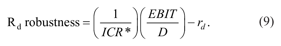
Another measure of robustness, which we call “R_d robustness,” indicates how much an increase in the cost of borrowing the firm could afford and yet still maintain its optimal rating:

R_{d} robustness = (\frac{1}{I C R *}) (\frac{E B I T}{D}) - r_{d} .

(9)

Graph 1 illustrates the concepts of financial flexibility and financial robustness. We implicitly assume that an ICR is the only key determinant of a credit rating. Given the cost of debt (r_d), we could plot the relationship between debt and minimum EBIT required to maintain the threshold ICR. The equation is as follows: EBIT = ICR*(r_d.D).

A derivation of all these measures is reported in Supplemental Appendix A-5.

Graph 1.

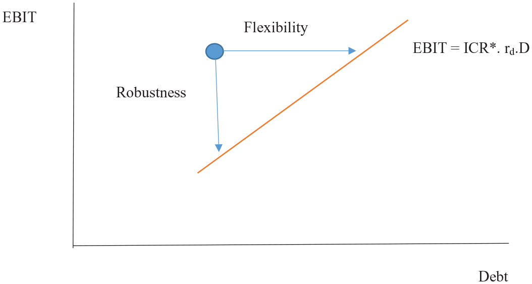
Relationship between credit rating, EBIT, and debt.

Finding the Optimal Capital Structure in a Case of a Constant Book-Value Debt Ratio With a Constant Growth

We apply the above framework to estimate the optimal capital structure of an average U.S. non-financial firm. The excel template file in this study can be used to search for the optimal capital structure by plugging in new data. The results reported in this study are also in this file. The file can be downloaded at https://drive.google.com/file/d/1exiFMAcbZbLfe1T67H-kfrYFe9kLx3zn/view?usp=sharing.

The IC is normalized to 100. We apply the average effective corporate income tax rate (across only money-making companies) (T) of 25.32% (Damodaran, 2019i). The ROIC is 14.1% (an average among non-financial sectors) (Damodaran, 2019d). This firm would generate next period NOPAT of 14.1 (NOPAT₁ = ROIC × IC = 14.1% × 100).

To keep growing at a constant growth rate (g), a fraction “RR” from NOPAT needs to be reinvested. A constant growth rate would equal to a multiplication between the ROIC and the RR. The average RR across non-financial sectors in the United States is around 58.8% (Damodaran, 2019d). Therefore, the constant growth rate (g) of an average non-financial firm in the United States should be around 8.29% (g = ROIC × RR = 14.1% × 0.588). We start this analysis with this rather high constant growth rate and then later we lower it to calibrate with observed numbers.

Since there is a need to reinvest to grow in this case, NOPAT is no longer FCFF like in the no growth case. The FCFF would equal to NOPAT multiplied by 1 minus the RR. The next period FCFF is 5.8, FCFF₁ = NOPAT₁.(1 – RR) = 14.1 × (1 – 0.588) = 5.8.

We use the risk-free rate (r_f) of 4.5% as suggested by Koller et al. (2015). They estimate this one from the expected inflation rate of 2.5% and the long-run average real interest rate of 2%. Although it differs from the actual yield, they argue that a current low interest rates is an aberration caused by the unorthodox monetary policy and a flight to safety.

We apply the unlevered beta corrected for cash (β_u) of 1 for an average U.S. non-financial firm (Damodaran, 2019f) and the MRP of 5.96% (Damodaran, 2019b). The unlevered cost of equity (r_u) is 10.46%, r_u = r_f + β_u.MRP = 4.5% + (1) × (5.96%), according to the CAPM. The unlevered cost of capital (WACC) would also equal to the unlevered cost of equity (r_u) at 10.46%. The unlevered value of the firm (V_u) would equal to FCFF₁/(WACC – g) in this constant growth case. So, the unlevered value of the firm would equal to 267.7, V_u = 5.8/(10.46% – 8.29%) = 267.7.

To capture the impact of credit risk on the cost of debt, we follow Damodaran (2012) in using credit rating as a key determinant of a spread above a risk-free rate. We apply the historical relationship between ICRs (EBIT/I), credit ratings, and default spreads (Damodaran, 2019h) as reported in Table 1.

The interest expense would equal to the cost of debt (r_d = r_f + spread) times the amount of debt (D). The spread is determined by the firm’s credit rating which in turns is determined by EBIT over the interest expense (I) itself. In addition, the amount of debt (D) is a multiplication between market-value debt ratio (W_d) and value of the firm (V). However, to get the value of the firm, we need the cost of debt first to calculate WACC. We also need the interest expense (I) as a multiplication between the amount of debt (D) and the cost of debt (r_d). There is a circularity here. We solve the problem by recursively iterating the process until it converges.

Table 2 shows how to find an optimal book-value debt ratio in the case of constant growth with the Hamada equation that incorporates credit risk. In this case, we use the modified Hamada equation to calculate levered beta according to β_l = (1 + [1 – T].[D*/E]).β_u. We increase the market-value debt ratio (W_d) with an increment of 5 percentage-point each step. The optimal W_d is found at 10% with the minimum WACC of 10.33% and the maximum firm value (V) of 285.5, V₀ = FCFF₁/(WACC – g) = 5.8/(10.33% – 8.29%) = 285.5. The optimal credit rating is “AAA.” Admittedly, this credit rating is obviously too high for an average firm. The optimal market-value D/E is 0.11 (W_d/W_e = 10%/90%). The market-value and also the book-value of debt is 28.5 (10% × 285.5). Given the IC of 100, this implies that the book-value of equity is 71.5 (100 – 28.5). The book-value debt ratio (BW_d) is 29% (28.5/100), which is much higher than 10%, the market-value one. Also, the D/BE is 0.40 (28.5/71.5) higher than the market-value one (D/E) at 0.11. Given that price-to-book ratio (PBV) is higher than one (PBV = E/BE = 256.9/71.5 = 3.60), the book-value debt ratio would be higher than the market-value one.

Table 2.

Optimal Book-Value Debt Ratio in the Case of a Constant Growth at 8.29%.

(0)	(1)	(2)	(3)	(4)	(5)	(6)	(7)	(8)	(9)	(10)	(11)	(12)	(13)	(14)	(15)	(16)	(17)	(18)	(19)	(20)	(21)	(22)
	BD	28.5	NOPAT	14.1	T	25.32%	BetaU	1	B W_d	28.5%	WACC	10.3%
	BE	71.5	EBIT	18.9	Rf	4.5%	MRP	5.96%	B We	71.5%	Rating	AAA
	IC	100.0	RR	58.8%	Rd	5.25%	Growth	8.29%	B DE	0.40	E	256.9
	ROIC	14.1%	FCFF	5.8	Re	11.04%	FCFE	7.06	Net Borrow	2.4	FCFE	7.06
	NI	13.0	Net Invest	8.3	T applied	25.32%	I	1.50
B W_d (%)	W_d (%)	D	I	ICR	Rating	Rd (%)	Tax rate (%)	Rd(1 – T) %	We (%)	D/E	D*	D*/E	Beta	Re (%)	WACC (%)	V	E	NI	BE	D/BE	E/BE	ROE (%)
0	0	—	0.0000	Inf	AAA	5.25	25.32	3.92	100	0.00	—	0.00	1.0	10.46	10.46	267.7	267.7	14.1	100.0	0.00	2.68	14.1
14	5	13.8	0.7253	26.03	AAA	5.25	25.32	3.92	95	0.05	16.1	0.06	1.0	10.73	10.39	276.3	262.5	13.6	86.2	0.16	3.05	15.7
29	10	28.5	1.4986	12.60	AAA	5.25	25.32	3.92	90	0.11	33.3	0.13	1.1	11.04	10.33	285.5	256.9	13.0	71.5	0.40	3.60	18.2
42	15	41.5	2.3883	7.91	A+	5.75	25.32	4.29	85	0.18	53.1	0.23	1.2	11.46	10.39	276.9	235.4	12.3	58.5	0.71	4.03	21.1
53	20	53.3	3.2273	5.85	A–	6.06	25.32	4.53	80	0.25	71.7	0.34	1.3	11.96	10.47	266.3	213.0	11.7	46.7	1.14	4.56	25.0
66	25	66.5	4.0287	4.69	A–	6.06	25.32	4.53	75	0.33	89.5	0.45	1.3	12.46	10.47	265.9	199.4	11.1	33.5	1.98	5.95	33.1
72	30	72.1	4.6874	4.03	BBB	6.50	25.32	4.85	70	0.43	104.2	0.62	1.5	13.22	10.71	240.4	168.3	10.6	27.9	2.59	6.03	38.0
66	35	66.3	4.9748	3.80	BB+	7.50	25.32	5.60	65	0.54	110.6	0.90	1.7	14.45	11.36	189.5	123.2	10.4	33.7	1.97	3.66	30.8
64	40	72.8	5.4576	3.46	BB	8.10	25.32	6.05	60	0.67	131.0	1.20	1.9	15.80	11.90	160.9	88.2	10.0	27.2	2.67	3.24	36.8
69	45	69.0	5.5872	3.38	BB	8.10	25.32	6.05	55	0.82	124.2	1.47	2.1	17.02	12.08	153.3	84.3	9.9	31.0	2.22	2.72	32.0

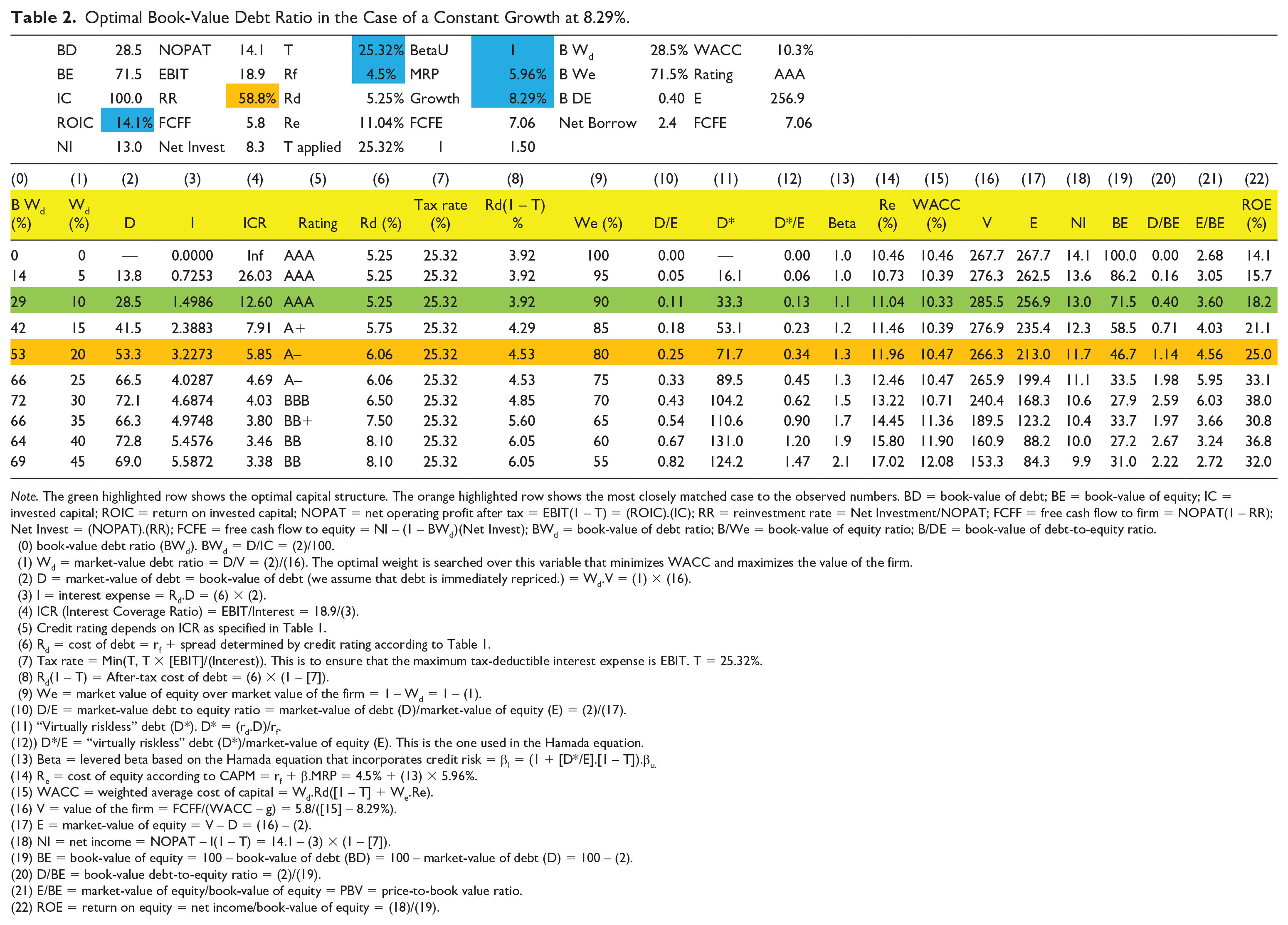
Note. The green highlighted row shows the optimal capital structure. The orange highlighted row shows the most closely matched case to the observed numbers. BD = book-value of debt; BE = book-value of equity; IC = invested capital; ROIC = return on invested capital; NOPAT = net operating profit after tax = EBIT(1 – T) = (ROIC).(IC); RR = reinvestment rate = Net Investment/NOPAT; FCFF = free cash flow to firm = NOPAT(1 – RR); Net Invest = (NOPAT).(RR); FCFE = free cash flow to equity = NI – (1 – BW_d)(Net Invest); BW_d = book-value of debt ratio; B/We = book-value of equity ratio; B/DE = book-value of debt-to-equity ratio.

(0) book-value debt ratio (BW_d). BW_d = D/IC = (2)/100.

(1) W_d = market-value debt ratio = D/V = (2)/(16). The optimal weight is searched over this variable that minimizes WACC and maximizes the value of the firm.

(2) D = market-value of debt = book-value of debt (we assume that debt is immediately repriced.) = W_d.V = (1) × (16).

(3) I = interest expense = R_d.D = (6) × (2).

(4) ICR (Interest Coverage Ratio) = EBIT/Interest = 18.9/(3).

(5) Credit rating depends on ICR as specified in Table 1.

(6) R_d = cost of debt = r_f + spread determined by credit rating according to Table 1.

(7) Tax rate = Min(T, T × [EBIT]/(Interest)). This is to ensure that the maximum tax-deductible interest expense is EBIT. T = 25.32%.

(8) R_d(1 – T) = After-tax cost of debt = (6) × (1 – [7]).

(9) We = market value of equity over market value of the firm = 1 – W_d = 1 – (1).

(10) D/E = market-value debt to equity ratio = market-value of debt (D)/market-value of equity (E) = (2)/(17).

(11) “Virtually riskless” debt (D*). D* = (r_d.D)/r_f.

(12)) D*/E = “virtually riskless” debt (D*)/market-value of equity (E). This is the one used in the Hamada equation.

(13) Beta = levered beta based on the Hamada equation that incorporates credit risk = β_l = (1 + [D*/E].[1 – T]).β_u.

(14) R_e = cost of equity according to CAPM = r_f + β.MRP = 4.5% + (13) × 5.96%.

(15) WACC = weighted average cost of capital = W_d.Rd([1 – T] + W_e.Re).

(16) V = value of the firm = FCFF/(WACC – g) = 5.8/([15] – 8.29%).

(17) E = market-value of equity = V – D = (16) – (2).

(18) NI = net income = NOPAT – I(1 – T) = 14.1 – (3) × (1 – [7]).

(19) BE = book-value of equity = 100 – book-value of debt (BD) = 100 – market-value of debt (D) = 100 – (2).

(20) D/BE = book-value debt-to-equity ratio = (2)/(19).

(21) E/BE = market-value of equity/book-value of equity = PBV = price-to-book value ratio.

(22) ROE = return on equity = net income/book-value of equity = (18)/(19).

As the firm grows at the constant rate and if other key variables (e.g., ROIC, r_f, spread, MRP) are constant, firm value and both market-value and book-value of debt would grow at the same constant rate (g). Therefore, the optimal book-value debt ratio would remain stable (see Supplemental Appendix A-8).

Our estimated optimal book-value debt ratio (BW_d) of an average U.S. non-financial firm is 29% and the market-value one (W_d) is 10%. These compare to the observed average book-value and market-value debt ratio of 49.71% and 25.66%, respectively (Damodaran, 2019c). Similarly, our estimated optimal book-value and market-value debt-to-equity ratio (D/BE and D/E) are 0.40 and 0.11, respectively. These compare to the observed ones of 1 and 0.3451, respectively (Damodaran, 2019c). Our estimated optimal PBV (E/BE) is at 3.60 compared to the observed one at 3.18 (Damodaran, 2019g).

Our estimated optimal book-value debt ratio (BW_d) of an average U.S. non-financial firm is quite different from the observed one (29% compared to the observed one at 49.71%). In fact, the book-value debt ratio of 53% is our closest case to the observed number of 49.71%. The credit rating is also more reasonable at “A–.” However, the market-value debt ratio of 20% still quite differs from the observed one at 25.66% and the price-to-book value ratio (PBV or E/BE) is still too high at 4.56 times compared to the observed one at 3.18 times.

It is notable that the cost of capital (WACC) is relatively flat around the optimal capital structure. A deviation from the optimal book-value (market-value) debt ratio of 29% (10%) to our closest case of 53% (20%) would lead to an increase in WACC of only 14 basis points (0.14% = 10.47% – 10.33%). Given the fact that a firm tends to adjust its capital structure gradually over time, it is conceivable that in the past the optimal book-value debt ratio (BW_d) was higher. Before the Trump’s tax cut of 2017, the corporate income tax rate in the United States was much higher at 35%. In our model, if we increase the tax rate (T) to 35%, then our estimated optimal book-value debt ratio (BW_d) would increase drastically from of 30% to 79%. Admittedly, the ratio is unrealistically high, but it points out the clear direction. Higher tax rate in the past and slow adjustment speed could partially explain why our optimal ratio is lower than the observed one.

To better calibrate our model to the observed numbers, we vary only one variable, namely, the perpetual growth rate (g). We lower it from an unusual high constant growth of 8.29% (Damodaran, 2019d) to 7.00%. This is about the same as analyst growth estimate of 7.05% in 2017 (Damodaran, 2019e). In fact, any growth rate in between 6.70% to 7.00% would provide about the same qualitative results. The RR is adjusted accordingly from 58.8% to 49.6% (RR = g/ROIC = 7%/14.1% = 0.496). The results are reported in Table 3.

Table 3.

Optimal Book-Value Debt Ratio in the Case of a Constant Growth at 7%.

(0)	(1)	(2)	(3)	(4)	(5)	(6)	(7)	(8)	(9)	(10)	(11)	(12)	(13)	(14)	(15)	(16)	(17)	(18)	(19)	(20)	(21)	(22)
	BD	32.0	NOPAT	14.1	T	25.32%	BetaU	1	B W_d	32.0%	WACC	10.3%
	BE	68.0	EBIT	18.9	Rf	4.5%	MRP	5.96%	B We	68.0%	Rating	AA
	IC	100.0	RR	49.6%	Rd	5.50%	Growth	7.00%	B DE	0.47	E	181.6
	ROIC	14.1%	FCFF	7.1	Re	11.42%	FCFE	8.03	Net Borrow	2.2	FCFE	8.03
	NI	12.8	Net Invest	7.0	T applied	25.32%	I	1.76
B W_d %	W_d %	D	I	ICR	Rating	Rd %	Tax rate %	Rd(1 – T) %	We %	D/E	D*	D*/E	Beta	Re %	WACC %	V	E	NI	BE	D/BE	E/BE	ROE %
0	0	—	0.0000	Inf	AAA	5.25	25.32	3.92	100	0.00	—	0.00	1.0	10.46	10.46	205.2	205.2	14.1	100.0	0.00	2.05	14.1
10	5	10.5	0.5493	34.37	AAA	5.25	25.32	3.92	95	0.05	12.2	0.06	1.0	10.73	10.39	209.3	198.8	13.7	89.5	0.12	2.22	15.3
21	10	21.4	1.1209	16.84	AAA	5.25	25.32	3.92	90	0.11	24.9	0.13	1.1	11.04	10.33	213.5	192.2	13.3	78.6	0.27	2.44	16.9
32	15	32.0	1.7627	10.71	AA	5.50	25.32	4.11	85	0.18	39.2	0.22	1.2	11.42	10.32	213.7	181.6	12.8	68.0	0.47	2.67	18.8
42	20	42.2	2.4270	7.78	A+	5.75	25.32	4.29	80	0.25	53.9	0.32	1.2	11.88	10.36	211.0	168.8	12.3	57.8	0.73	2.92	21.3
52	25	52.3	3.0726	6.14	A	5.88	25.32	4.39	75	0.33	68.3	0.44	1.3	12.40	10.40	209.0	156.8	11.8	47.7	1.09	3.28	24.7
61	30	61.2	3.7114	5.09	A–	6.06	25.32	4.53	70	0.43	82.5	0.58	1.4	13.03	10.48	204.1	142.9	11.3	38.8	1.58	3.69	29.2
66	35	66.3	4.3094	4.38	BBB	6.50	25.32	4.85	65	0.54	95.8	0.78	1.6	13.92	10.75	189.4	123.1	10.9	33.7	1.97	3.65	32.3
63	40	63.3	4.7506	3.97	BB+	7.50	25.32	5.60	60	0.67	105.6	1.11	1.8	15.41	11.48	158.4	95.0	10.6	36.7	1.73	2.59	28.8
69	45	69.3	5.1961	3.63	BB+	7.50	25.32	5.60	55	0.82	115.5	1.36	2.0	16.53	11.61	154.0	84.7	10.2	30.7	2.26	2.76	33.3

(0) Book-value debt ratio (BW_d).BW_d = D/IC = (2)/100.

(1) W_d = market-value debt ratio = D/V = (2)/(16). The optimal weight is searched over this variable that minimizes WACC and maximizes the value of the firm.

(2) D = market-value of debt = book-value of debt (we assume that debt is immediately repriced.) = W_d.V = (1) × (16).

(3) I = interest expense = R_d.D = (6) × (2).

(4) ICR (Interest Coverage Ratio) = EBIT/Interest = 18.9/(3).

(5) Credit rating depends on ICR as specified in Table 1.

(6) R_d = cost of debt = r_f + spread determined by credit rating according to Table 1.

(7) Tax rate = Min(T, T × [EBIT]/(Interest)). This is to ensure that the maximum tax-deductible interest expense is EBIT.T = 25.32%.

(8) R_d(1 – T) = After-tax cost of debt = (6) × (1 – [7]).

(9) We = market value of equity over market value of the firm = 1 – W_d = 1 – (1).

(10) D/E = market-value debt to equity ratio = market-value of debt (D)/market-value of equity (E) = (2)/(17).

(11) “Virtually riskless” debt (D*). D* = (r_d.D)/r_f.

(12)) D*/E = “virtually riskless” debt (D*)/market-value of equity (E) This is the one used in the Hamada equation.

(13) Beta = levered beta based on the Hamada equation that incorporates credit risk = β_l = (1 + [D*/E].[1 – T]).β_u.

(14) R_e = cost of equity according to CAPM = r_f + β.MRP = 4.5% + (13) × 5.96%.

(15) WACC = weighted average cost of capital = W_d. Rd([1 – T] + W_e.Re).

(16) V = value of the firm = FCFF/(WACC – g) = 5.8/([15] – 8.29%).

(17) E = market-value of equity = V – D = (16) – (2).

(18) NI = net income = NOPAT – I(1 – T) = 14.1 – (3) × (1 – [7]).

(19) BE = book-value of equity = 100 – book-value of debt (BD) = 100 – market-value of debt (D) = 100 – (2).

(20) D/BE = book-value debt-to-equity ratio = (2)/(19).

(21) E/BE = market-value of equity/book-value of equity = PBV = price-to-book value ratio.

(22) ROE = return on equity = net income/book-value of equity = (18)/(19).

With lower growth, our optimal book-value (market-value) debt ratio increases from 29% (10%) to 32% (15%). It is closer to the observed book-value (market-value) ratio of 49.71% (25.66%). Again, the cost of capital (WACC) is relatively flat around the optimal capital structure. The most closely matched case to the observed numbers is at the book-value debt ratio (BW_d) of 52%. The WACC increases from our optimal one by only eight basis points (0.08% = 10.40% - 10.32%).

At this almost optimal book-value debt ratio (BW_d) of 52%, our numbers match observed numbers quite closely. Our book-value (market-value) debt ratio is 52% (25%) compared to the observed number of 49.71% (25.66%) (Damodaran, 2019c). Similarly, our book-value (market-value) debt-to-equity ratio is 1.09 (0.33) compared to the observed number of 1 (0.3451) (Damodaran, 2019c). Our price-to-book value ratio (PBV = E/BE) is 3.28 compared to the observed number at 3.18 (Damodaran, 2019g). Given that price-to-book ratio (PBV) is higher than 1, the book-value debt ratio would be higher than the market-value one. This is typically the case when the return on equity (ROE) is higher than the cost of equity (r_e) (see Supplemental Appendix A-8).

The credit rating is more reasonable for an average firm at a single “A.” The majority (about 75%) of big companies (with market capitalization more than $5 billion) are in the rating class of A+ to BBB–. If we expand our samples to companies with market capitalization more than $1 billion, then about 53% are in theses rating categories (Koller et al., 2015).

However, our model produces costs of fund for an average firm that are higher than the observed ones (Damodaran, 2019a). Our cost of debt is 5.88% compared to 4.56% (observed). Our cost of equity is 12.40% compared to 9.87 (observed). Our cost of capital (WACC) is 10.40% compared to 8.22% (observed). Nevertheless, our estimated beta of 1.3 is close to the observed one at 1.21 (Damodaran, 2019a).

Table 4 reports the financial robustness and financial flexibility in the case of a constant growth at 7%. It shows that at the optimal book-value debt ratio of 32% and the corresponding market-value debt ratio of 15%. To maintain the rating at “AA” the firm needs to keep its ICR at least at the threshold ICR (ICR*) of 9.50 while the ICR at the optimal debt is at 10.71. The amount that the firm could borrow more and maintain its credit rating is (EBIT/r_d)(1/ICR* – 1/ICR) = (18.9/5.50%)(1/9.50 – 1/10.71) = 4.09. This simply means that the firm could increase its debt by about 13% (flexibility/book-value of debt = 4.09/32), and yet still maintain its rating and it uses about 89% (32/36.14) of its debt capacity (debt capacity = book-value of debt + flexibility = 32 + 4.09 ≈ 36.14) at this rating.

Table 4.

Financial Robustness and Financial Flexibility in the Case of a Constant Growth at 7%.

Measures	Values	% Change allowed	% of Debt capacity used	Debt capacity
Financial flexibility	4.09	+13% (Debt)	89%	36.14
Financial robustness	2.14	−11% (EBIT)
Rd robustness	0.7%
Benefits: Flexibility	Flexibility	1.0
	Robustness	0.5
	Rd robust	0.2%
Costs: Loss in Tax Saving	Loss TS	−0.25

The robustness is measured by how much EBIT could drop before its ICR would be below the minimum to maintain its credit rating (9.50 in this case). The formula is EBIT – ICR*.r_d.D. In this case, it is 18.9 – (9.50)(5.50%)(32) ≈ 2.14. The numbers are not exact due to rounding errors. This simply means that the firm could afford to have a lower EBIT by 11% (robustness/EBIT = 2.14/18.9) and yet still maintain its optimal credit rating.

Another measure of robustness, which we call “Rd robustness,” indicates how much an increase in the cost of borrowing the firm could afford and yet still maintain its optimal rating. The formula is (1/ICR*).(EBIT/D) – r_d. It is 0.7%, (1/9.50).(18.9/32) – 5.50%, in this case.

By lowering its debt by one unit, a firm could increase its flexibility by 1, its robustness by 0.5 (ICR*.r_d = [9.5] × [5.50%]), and its Rd robustness by 0.2% ([(1/ICR*) × (EBIT/[D – 1]) – r_d] – [(1/ICR*) × (EBIT/D) – r_d ] = [(1/9.50) × (18.9/(32 – 1)] – 5.50%] – [(1/9.50) × (18.9/(32)] – 5.50%] = 0.2%). The cost in terms of a loss in tax-saving is –0.25 (–T). A financial manager can weight this loss in tax-saving with the gains in terms of financial robustness and financial flexibility.

Sensitivity Analysis

We vary one key variable at a time whereas all other variables are at their default values as reported in Table 3. Supplemental Appendix A-13 extends this analysis further by performing scenario analysis.

Corporate Income Tax Rate (T)

When we vary “T,” we also indirectly vary “ROIC” simultaneously. Since ROIC is the after-tax ROIC, when a tax rate changes, then ROIC will also change. We adjust ROIC using the above default values according to the following equations:

\begin{array}{l} R O I C_{after tax} = \frac{N O P A T}{I C} = \frac{E B I T (1 - T)}{I C} \\ = \frac{E B I T}{I C} . (1 - T) = R O I C_{before tax} . (1 - T), \\ 14.1 % = R O I C_{before tax} . (1 - 25.32 %), \\ R O I C_{before tax} = \frac{14.1 %}{(1 - 25.32 %)}, \\ R O I C_{after tax} = R O I C_{before tax} . (1 - T) \\ = \frac{14.1 %}{(1 - 25.32 %)} . (1 - T) . \end{array}

(10)

In Graph 2, we plot relationships between corporate income tax rate (T), market-value debt ratio (W_d), book-value debt ratio (BW_d), and cost of capital (WACC). The detailed data are reported in Table A7 in the Supplemental Appendix. As predicted by the capital structure theory (Modigliani & Miller, 1958), a higher corporate income tax rate would mean a higher tax-saving from debt financing. This tax-saving benefit would lower the cost of capital. As a tax rate increases, the WACC will go down. We also find that an increase in a tax rate (T) would lead to higher optimal market-value and higher optimal book-value debt ratios.

Graph 2.

Relationships between corporate income tax rate (T), optimal market-value debt ratio (Wd), optimal book-value debt ratio (B Wd), and cost of capital (WACC).

In fact, if a corporate income tax rate is too low (in this case when T ≤ 14%), then it is optimal to be an unleveraged (0 debt) firm. The underlying logic is that if a tax rate is low, then the benefit from interest tax-saving is also low. A firm logically compares this lower benefit to a cost in the form of a spread over the risk-free rate. Even when a firm has a very low amount of debt and gets the “AAA” rating, it still needs to pay a spread over a risk-free rate (0.75% in this case). This minimum spread acts as a fixed cost of using leverage. Therefore, if the benefit from interest tax-saving is not high enough, then it is better to be unleveraged.

Once a tax rate is higher than a threshold level (14% in this case), optimal debt ratios would jump drastically to around 10% for market-value debt ratio (W_d) and 25% for book-value debt ratio (BW_d). Both the market-value debt ratio and the book-value debt ratio increase slowly but steadily with a tax rate. Both debt ratios jump drastically again when a tax rate reaches 30%. The underlying logic of this second jump is basically the same as the first one. As a tax rate increases, a firm would like to take more advantage from a debt tax shield, but it also does not want to lower its credit rating and pay a higher spread. In this case, a spread would increase by 0.25% from a “AAA” rating to a “AA” rating. Once a tax rate is high enough to generate enough tax-saving benefit compared to a cost, a firm would be willing to pay a price of lower credit rating and a higher spread. After paying this fixed price, a firm would like to take as much tax-saving benefit as it could by borrowing much more and increase its debt ratios drastically.

Jong et al. (2008) study determinants of corporate leverage from 42 countries and observe that corporate taxation yields statistically significant coefficients only in 10 countries. In addition, only 2 out of 10 significant coefficients are positive. They explain that the reason why most studies fail to find significant tax effects on leverage is because the debt-to-equity ratios are cumulative result of years of separate decisions and tax shield have a negligible effect on the marginal tax rate for most firms (MacKie-Mason, 1990).

Our results are compatible with the results from Jong et al. (2008) in a sense that for certain ranges of tax rate, for example, 0%–14% or 14%–30%, tax rates have minimal impacts on leverage. A corporate income tax rate would have a huge impact on leverage only when it crosses certain thresholds in this case 14% and 30%. Our model helps explain the rationales behind empirical results found in existing literature that a tax variable often yields an insignificant coefficient.

Growth Rate (g)

Graph 3 plots relationships between perpetual growth rate (g), market-value debt ratio (W_d), book-value debt ratio (BW_d), and cost of capital (WACC). The detailed data are reported in Table A8 in the Supplemental Appendix. As the growth rate increases, the cost of capital also steadily increases but very slowly. It ranges from 10.19% to 10.43% as “g” varies from 0% to 10%. This is the result of a lower financing from debt (lower W_d) and a higher financing from equity (higher W_e). In our case, W_d decreases drastically from 20% to 3% as the growth rate increases from 0% to 10%. Since the cost of equity (r_e) is higher than the cost of debt (r_d), more financing from equity would increase the cost of capital. In contrast, the book-value debt ratio (BW_d), though not a constant, remains very stable at around 27.7%, varying from 26.1% to 28.5%. Notably, it does not have a clear directional relationship with a perpetual growth rate.

Graph 3.

Relationships between perpetual growth rate (g), optimal market-value debt ratio (Wd), optimal book-value debt ratio (B Wd), and cost of capital (WACC).

The key question is then what explains a lower proportion of debt financing or lower market-value debt ratio (lower W_d) as a growth rate increases. Equivalently, the question is why a firm use more equity financing (higher W_e) as it has a higher growth rate. The rationale is quite subtle.

A higher perpetual growth rate (g) would lead to a higher firm value (V) through the equation, V₀ = FCFF₁/(WACC – g). At the same market-value debt ratio (W_d), a higher value would imply a higher amount of debt as, D = W_d × V. Of course, a higher amount of debt would mean a higher interest payment (I). Given a constant ROIC and a constant initial EBIT (EBIT₁ = ROIC × IC₀), a higher interest (I) would mean a lower ICR (ICR = EBIT/I). Since a credit rating is mainly determined by ICR, a significant lower ICR would mean a credit downgrade. This lower credit rating would lead to a higher credit spread and a higher cost of debt (r_d).

However, it is not just because of this higher cost of debt that a firm decides to finance more from equity. The reason is that the cost of equity at the corresponding “W_e” (W_e = 1 – W_d) also increases. So, it is not obvious why a firm would switch more to equity financing. The cost of equity, itself, increases due to a higher beta. The next logical question is then why beta would increase. We need to refer to our modified Hamada equation here:

\begin{array}{l} β_{l} = β_{u} [1 + \frac{D^{*}}{E} (1 - T)], where D^{*} = \frac{r_{d} . D}{r_{f}}, \\ β_{l} = β_{u} [1 + (\frac{r_{d}}{r_{f}}) (\frac{D}{E}) (1 - T)], \end{array}

(11)

where the risk-free rate (r_f) and corporate income tax rate (T) are constant. In addition, the market debt-to-equity ratio (D/E) would also be constant at any level of “W_d” or “W_e” because it is simply equal to W_d/W_e and the fact that W_d + W_e = 1.

An increase in the cost of debt (r_d) from a lower credit rating would increase beta and subsequently the cost of equity (r_e) through the CAPM equation (r_e = r_f + β_l.MRP). However, increases in r_d, β_l, and r_e are much lower when a firm has a lower market-value debt ratio (W_d) or, equivalently, a higher market-value equity ratio (W_e). The reason is that a low “W_d” even when multiplied by a higher firm value (V) caused by a higher growth rate will result in at most a modest increase in the amount of debt (D) and at most a small increase in interest (I). As such, the ICR is not significantly affected. Because of this stable ICR, the rating is maintained, and a firm does not have to pay a higher credit spread. This, in the end, results in at most a very modest increase in the cost of equity (r_e).

In summary, a higher perpetual growth rate (g) would lead to a much higher firm value (V). Given the same “W_d,” the amount of debt and interest payment will increase so much that a firm faces a possible credit rating downgrade. Such a downgrade would lead to a higher cost of debt (r_d) and a higher cost of equity (r_e) through the modified Hamada equation. That would result in a steep increase in WACC. In response, a firm would finance less by debt (lower W_d) to limit a rapid increase in the amount of debt and a chance of a downgrade and, at the same time, finance more by equity (higher W_e). At this higher level of “W_e,” the cost of equity (r_e) is much less affected by an increase in a perpetual growth rate (g). However, as the cost of equity (r_e) is always higher than the cost of debt (r_d), more financing from equity would lead to a higher cost of capital (WACC). That is the reason why, in Graph 3, WACC is an increasing function of a perpetual growth rate (g).

The effect of an increase in growth rate on the optimal book-value debt ratio (BW_d) is the net effect of two opposing forces. The first one is a higher firm value resulted from a higher growth rate. This would lead to a higher amount of debt (D) given the same market-value of debt (W_d) and a higher book-value debt ratio (BW_d). The second one is a lower optimal market-value of debt (W_d) due to a mechanic explained above. These two opposing forces cancel each other mostly. That is the reason why we see that the optimal book-value debt ratio (BW_d) is quite stable as a perpetual growth rate (g) increases.

Concerning market debt ratios, our results exactly match the consensus finding that there is a negative relationship with growth opportunities (e.g., Fama and French, 2002; Gul, 1999; Jong et al., 2008). Concerning book debt ratios, there is no consensus among existing empirical studies. Most studies find that the coefficients are insignificant (Gul, 1999) or give conflicting results (Fama & French, 2002). Our results match theirs and offer the explanation. Supplemental Appendix A-11 provides detailed literature review on this relationship and compare existing studies with our results.

Risk-Free Rate (r_f)

Graph 4 plots the relationships between risk-free rate (r_f), market-value debt ratio (W_d), book-value debt ratio (BW_d), and cost of capital (WACC). The detailed data are reported in Table A9 in the Supplemental Appendix. A cost of capital increases almost linearly with a risk-free rate. It ranges from 9.13% to 11.68% as “r_f” rises from 3.25% to 6.00%. A rise in “r_f” would simultaneously raises both the cost of debt (r_d) and the cost of equity (r_e), resulting in a higher cost of capital.

Graph 4.

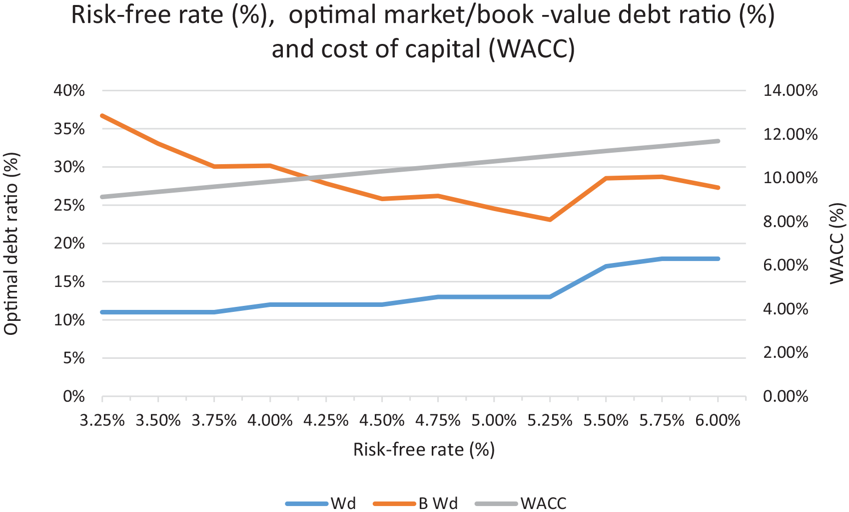
Relationships between risk-free rate (r_f), optimal market-value debt ratio (Wd), optimal book-value debt ratio (B Wd), and cost of capital (WACC).

As a result of a higher WACC, the firm’s value (V) will go down. So, at the same market-value debt ratio (W_d), the amount of debt (D) will also go down. To compensate, a firm could afford to increase “W_d” to maximize its tax-saving benefit but still maintain its optimal credit rating. This explains why “W_d,” for a large part, increases gradually as “r_f” increases.

Within the same credit rating, an increase in risk-free rate would increase the cost of debt on the one-to-one basis as “r_d = r_f + spread.” Although the cost of equity also increases as “r_e = r_f + β.MRP,” it increases at a slower rate than the one-to-one basis. The reason is that β will be lower due to the following equation:

\begin{array}{l} β_{l} = β_{u} [1 + (\frac{r_{d}}{r_{f}}) (\frac{D}{E}) (1 - T)], \\ = β_{u} [1 + (\frac{r_{f} + s p r e a d}{r_{f}}) (\frac{D}{E}) (1 - T)], \end{array}

(12)

here, since (r_f + spread)/r_f is higher than 1, a one unit increase of r_f would increase both numerator and denominator by the same unit, but it will lower this ratio and the leveraged beta. Therefore, the cost of equity would increase less than a one unit increase in a risk-free rate.

Moreover, at a lower credit rating (higher credit spread), this ratio will decrease at a faster rate than at a higher credit rating. This implies a smaller increase in the cost of equity for lower credit rating firms. Therefore, after a risk-free rate rises to a certain point, the optimal credit rating will go down. After paying a fixed cost in the form of a higher credit spread due to lower rating, a firm would just borrow as much as it could as long as it could still maintain its new optimal rating (see Graph 4 at r_f = 5.5%). That explains why the market-value debt ratio (W_d) would jump up when a risk-free rate increases to a certain extent and its optimal credit rating decreases.

The book-value debt ratio (BW_d) decreases as a risk-free (r_f) continues to rise. This is mainly due to the valuation effect. As WACC increases following a rise in “r_f,” the firm’s value will go down. This leads to a lower amount of debt (D), although a firm tries to compensate by increasing its market-value debt ratio (W_d). However, when the lower credit rating becomes optimal, a firm would drastically increase its “W_d.” That leads to a higher amount of debt as an increase in “W_d” is more than enough to compensate for the valuation effect. That explains why the book-value debt ratio increases when the optimal credit rating changes from “AAA” to “AA” when “r_f” increases from 5.25% to 5.50%.

Previous empirical literature still gives conflicting results on the impact of interest rate on capital structure. Bokpin (2009) finds that it has significant positive relationships with external financing and short-term debt to total assets. In contrast, Dincergok and Yalciner (2011) argue that interest rate has a negative relationship with capital structure.

Return on Invested Capital (ROIC)

Graph 5 plots relationships between ROIC, market-value debt ratio (W_d), book-value debt ratio (BW_d), and cost of capital (WACC). The detailed data are reported in Table A10 in the Supplemental Appendix. The market-value debt ratio (W_d) steadily decreases as ROIC increases. In sharp contrast, the book-value debt ratio (BW_d) tends to increase with ROIC. This graph illustrates clearly that market-value and book-value debt ratios do not necessary move in the same direction.

Graph 5.

Relationships between ROIC, optimal market-value debt ratio (Wd), optimal book-value debt ratio (B Wd), and cost of capital (WACC).

The cost of capital (WACC) increases slowly but steadily with ROIC. As ROIC rises from 7.5% to 20.0%, WACC increases marginally from 9.65% to 10.33%. Interestingly, within this range, there is no change in the cost of debt (r_d), which remains stable at 5.25%, and the cost of equity (r_e) actually decreases from 18.25% to 11.04%. The WACC increases mainly due to the switch from debt, which has a lower cost, to equity, which has a higher cost. The cost of equity (r_e) also decreases from this switching which lowers the market-value debt-to-equity ratio (D/E) and the leveraged beta (β_l).

The key question is then why a firm would switch from debt to equity when it has a higher ROIC. When ROIC increases, a firm value would increase drastically as shown in the following equations:

\begin{array}{l} N O P A T = R O I C \times I C, \\ R R = \frac{g}{R O I C}, \\ F C F F = N O P A T \times (1 - R R) \\ = R O I C \times I C \times (1 - \frac{g}{R O I C}), \\ V = \frac{F C F F}{(W A C C - g)} = \frac{R O I C \times I C \times (1 - \frac{g}{R O I C})}{(W A C C - g)} . \end{array}

(13)

At the same credit rating and market-value debt ratio (W_d), a higher firm value (V) would mean a higher amount of debt (D) and a higher interest payment (I = r_d.D). As the main determinant of credit rating is a firm’s ICR, a higher debt level would mean a lower ICR. We can link ICR and ROIC in the following equations:

\begin{array}{l} V = \frac{F C F F}{(W A C C - g)} = \frac{R O I C \times I C \times (1 - \frac{g}{R O I C})}{(W A C C - g)}, \\ I C R = \frac{E B I T}{I} = \frac{R O I C \times I C \times 1 / (1 - T)}{r_{d} \times w_{d} \times V}, \\ I C R = \frac{1 / (1 - T)}{r_{d} \times w_{d} \times (1 - \frac{g}{R O I C})}, \\ R O I C ⇑ \to I C R ⇓ . \end{array}

(14)

As shown above, an increase in ROIC would lower the ICR at every market-value debt ratio (W_d). To maintain the same optimal credit rating, a firm needs to lower its “W_d” to limit a jump in the debt level. As a result, a firm would optimally finance more by equity and less by debt to decrease its market-value debt ratio (W_d) when ROIC increases.

The book-value debt ratio (BW_d) is affected by two opposing forces. The first one is an increase in firm’s value (V) from a higher ROIC. This force will increase the amount of debt and the book-value debt ratio. The second one is a lower market-value debt ratio (W_d). This will lower the amount of debt given the firm’s value. So, it will decrease the book-value debt ratio. On balance, the first force tends to dominate and that is the reason why we see in the graph that the book-value debt ratio (BW_d) generally increases when ROIC increases. In this case, market-value and book-value debt ratios move in opposite directions.

With respect to market debt ratio, our results match the prediction of the pecking order theory. The trade-off theory does not give an unambiguous prediction. Our results are qualitatively similar to the findings by Fama and French (2002), Jong et al. (2008), and Antoniou et al. (2008).

With respect to book debt ratio, our results match the prediction of the trade-off theory and not the pecking order theory. Most studies (e.g., Fama and French, 2002; Rajan and Zingales, 1995, and Antoniou et al., 2008) find a negative relation between profitability and book debt ratio, whereas our results detect a positive one. However, most studies use past profitability as the explanatory variable when the trade-off theory focuses on expected future profitability. Our results use varying perpetual growth rates, which are more in line with the theory. That may explain the reason why our results match the prediction of the trade-off theory. Xu (2012), who uses import penetration as a proxy for future profitability, also finds similar results.

Supplemental Appendix A-12 provides detailed literature review on the relationship between profitability and debt ratios. It also compares existing studies with our results.

Discussion

We report our sensitivity results compared to theoretical predictions and existing empirical findings in Table 5. Overall, our results generally match the predictions of the existing theories and empirical findings. We even make new theoretical predictions with respect to the effect of a risk-free rate, although there is still no empirical consensus due to too few studies.

Table 5.

Comparisons of Our Results to Theoretical Predictions and Existing Empirical Findings.

Variables	Trade-off	Pecking order	Agency theory	Our model	Empirical findings
CIT tax rate
Market debt ratio	+	=	=	+stepwise	Mostly insignificantJong et al. (2008)
Book debt ratio	+	=	=	+stepwise	Mostly insignificantJong et al. (2008)
Growth rate
Market debt ratio	−	na	−	−	–Rajan & Zingales (1995) Jong et al. (2008) Antoniou et al. (2008)
Book debt ratio	−	+simple–complex	−	≈	–Rajan & Zingales (1995),Antoniou et al. (2008) ≈Gul (1999),Fama & French (2002)
Risk-free rate
Market debt ratio	na	na	na	+stepwise	Na
Book debt ratio	na	na	na	−generally	+Bokpin (2009) –Dincergok & Yalciner (2011)
Profitability
Market debt ratio	?	−	na	−	–Rajan & Zingales (1995),Fama & French (2002),Jong et al. (2008),Antoniou et al. (2008)
Book debt ratio	+	−	na	+	–Rajan & Zingales (1995),Fama & French (2002) +Xu (2012)

Note. CIT = corporate income tax; na = no prediction or no study; “?” ambiguous sign; “+” positive relationship; “–” negative relationship; “=” no relationship; “≈” approximately no relationship.

With respect to a corporate income tax rate, we predict a positive relationship with both market and book debt ratios similar to the trade-off model. In addition, we predict that it behaves in a stepwise fashion. That may help explain why empirical studies could not find a significant positive relationship.

With respect to a perpetual growth rate, we predict a negative relationship with a market debt ratio similar to both the trade-off model and the agency theory. The existing empirical studies also support this conclusion. However, we predict no clear directional relationship between growth and a book debt ratio dissimilar to existing theories. Some empirical studies support this result.

With respect to profitability, we predict a negative relationship with a market debt ratio similar to the pecking order theory. The existing empirical studies also support this conclusion. In contrast, we predict a positive relationship between growth and a book debt ratio similar to the trade-off model. Some empirical studies also find this result if they use expected future profitability instead of historical profitability.

Conclusion

The objective of this article is to provide a systematic and practical method to determine the optimal book-value debt ratio. We provide a practical, yet theoretically grounded, approach to estimate WACC and set the optimal capital structure. Our approach works even for non-listed firms with no observed market value. For listed firms, our approach can be used to estimate their target book debt ratios (Stowe et al., 2007) to be used in its financial planning and capital budgeting.

The limitation that we hope to relax further is the constant growth assumption. We would like to generalize the model on this aspect. In fact, we already extended our model to the case of zero growth in Supplemental Appendix A-10.

Supplemental Material

sj-docx-1-sgo-10.1177_2158244020985788 – Supplemental material for Optimal Book-Value Debt Ratio

Supplemental material, sj-docx-1-sgo-10.1177_2158244020985788 for Optimal Book-Value Debt Ratio by Piyapas Tharavanij in SAGE Open

Research Data

sj-xlsx-2-sgo-10.1177_2158244020985788 – Research Data for Optimal Book-Value Debt Ratio

Research Data, sj-xlsx-2-sgo-10.1177_2158244020985788 for Optimal Book-Value Debt Ratio by Piyapas Tharavanij in SAGE Open

This article is distributed under the terms of the Creative Commons Attribution 4.0 License (http://www.creativecommons.org/licenses/by/4.0/) which permits any use, reproduction and distribution of the work without further permission provided the original work is attributed as specified on the SAGE and Open Access pages (https://us.sagepub.com/en-us/nam/open-access-at-sage).

Footnotes

Declaration of Conflicting Interests

The author declared no potential conflicts of interest with respect to the research, authorship, and/or publication of this article.

Funding

The author received no financial support for the research, authorship, and/or publication of this article.

ORCID iD

Piyapas Tharavanij

Supplemental Material

Supplemental material for this article is available online.

References

Antoniou

Guney

Paudyal

(2008). The determinants of capital structure: Capital market-oriented versus bank-oriented institutions. Journal of Financial and Quantitative Analysis, 43(1), 59–92. https://www.jstor.org/stable/27647340

Bokpin

G. A.

(2009). Macroeconomic development and capital structure decisions of firms. Studies in Economics and Finance, 26(2), 129–142. https://doi.org/10.1108/10867370910963055

Cohen

R. D.

(2004, November). An analytical process for generating the WACC curve and locating the optimal capital structure. Wilmott Magazine. http://rdcohen.50megs.com/OCSabstract.htm

Cohen

R. D.

(2007, 27 September). Incorporating default risk into Hamada’s Equation for application to capital structure [MPRA paper]. https://mpra.ub.uni-muenchen.de/3190/

Conine

T. E.

Tamarkin

(1985). Divisional cost of capital estimation: Adjusting for leverage. Financial Management, 14(1), 54–58. https://www.jstor.org/stable/3665361

Damodaran

(2012). Investment valuation: Tools and techniques for determining the value of any asset (3rd ed.). John Wiley & Sons.

Damodaran

(2019a, January). Cost of capital by sector (U.S.). http://pages.stern.nyu.edu/~adamodar/New_Home_Page/datafile/wacc.htm

Damodaran

(2019b, January). Country default spreads and risk premiums. http://pages.stern.nyu.edu/~adamodar/New_Home_Page/datafile/ctryprem.html

Damodaran

(2019c, January). Debt fundamentals by sector (U.S.). http://pages.stern.nyu.edu/~adamodar/New_Home_Page/datafile/dbtfund.html

10.

Damodaran

(2019d, January). Fundamental growth in EBIT by sector (U.S.). http://pages.stern.nyu.edu/~adamodar/New_Home_Page/datafile/fundgrEB.html

11.

Damodaran

(2019e). Historical implied equity risk premiums. http://pages.stern.nyu.edu/~adamodar/New_Home_Page/datafile/histimpl.html

12.

Damodaran

(2019f). Levered and unlevered betas by industry (U.S.). http://www.stern.nyu.edu/~adamodar/pc/datasets/betas.xls

13.

Damodaran

(2019g, January). Price and value to book ratio by sector (U.S.). http://pages.stern.nyu.edu/~adamodar/New_Home_Page/datafile/pbvdata.html

14.

Damodaran

(2019h, January). Ratings, interest coverage ratios and default spread. http://pages.stern.nyu.edu/~adamodar/New_Home_Page/datafile/ratings.htm

15.

Damodaran

(2019i, January). Tax rates by sector (U.S.). http://pages.stern.nyu.edu/~adamodar/New_Home_Page/datafile/taxrate.htm

16.

Dincergok

Yalciner

(2011). Capital structure decisions of manufacturing firms’ in developing countries. Middle Eastern Finance and Economics, 12(7), 86–100.

17.

Fama

E. F.

French

K. R.

(2002). Testing trade-off and pecking order predictions about dividends and debt. Review of Financial Studies, 15(1), 1–33. https://www.jstor.org/stable/2696797

18.

Fernandez

(2007). A more realistic valuation: Adjusted present value and WACC with constant book leverage ratio. Journal of Applied Finance, 17(2), 13–20. https://ideas.repec.org/p/ebg/iesewp/d-0715.html

19.

Gul

F. A.

(1999). Growth opportunities, capital structure and dividend policies in Japan. Journal of Corporate Finance, 5(2), 141–168. https://doi.org/10.1016/S0929-1199(99)00003-6

20.

Hamada

R. S.

(1972). The effect of the firm’s capital structure on the systematic risk of common stocks. Journal of Finance, 27(2), 435–452. https://doi.org/10.2307/2978486

21.

Jong

d Kabir

Nguyen

T. T.

(2008). Capital structure around the world: The roles of firm- and country-specific determinants. Journal of Banking & Finance, 32(9), 1954–1969. https://doi.org/10.1016/j.jbankfin.2007.12.034

22.

Koller

Goedhart

Wessels

(2015). Valuation: Measuring and managing the value of companies (6th ed.). John Wiley & Sons.

23.

Kraus

Litzenberger

R. H.

(1973). A state-preference model of optimal financial leverage. Journal of Finance, 28(4), 911–922. https://doi.org/10.2307/2978343

24.

MacKie-Mason

J. K.

(1990). Do taxes affect corporate financing decisions? Journal of Finance, 45(5), 1471–1493. https://doi.org/10.2307/2328746

25.

Modigliani

Miller

M. H.

(1958). The cost of capital, corporation finance and the theory of investment. American Economic Review, 48(3), 261–296. www.jstor.org/stable/1809766

26.

Rajan

R. G.

Zingales

(1995). What do we know about capital structure? Some evidence from international data. Journal of Finance, 50(5), 1421–1460. https://doi.org/10.2307/2329322

27.

Stowe

J. D.

Robinson

T. R.

Pinto

J. E.

McLeavey

D. W.

(2007). Equity asset valuation. In CFA Institute (Ed.), CFA Institute investment series (p. 131). John Wiley & Sons.

28.

Welch

(2004). Capital structure and stock returns. Journal of Political Economy, 112(1), 106–131. https://www.jstor.org/stable/10.1086/379933

29.

(2012). Profitability and capital structure: Evidence from import penetration. Journal of Financial Economics, 106(2), 427–446. https://doi.org/10.1016/j.jfineco.2012.05.015

Supplementary Material

Please find the following supplemental material available below.

For Open Access articles published under a Creative Commons License, all supplemental material carries the same license as the article it is associated with.

For non-Open Access articles published, all supplemental material carries a non-exclusive license, and permission requests for re-use of supplemental material or any part of supplemental material shall be sent directly to the copyright owner as specified in the copyright notice associated with the article.

0.00 MB

0.27 MB

0.16 MB

Optimal Book-Value Debt Ratio

Abstract

Keywords

Introduction

Optimal Capital Structure in a Case of a Constant Book-Value Debt Ratio With a Constant Growth

Theoretical Model

Finding the Optimal Capital Structure in a Case of a Constant Book-Value Debt Ratio With a Constant Growth

Sensitivity Analysis

Corporate Income Tax Rate (T)

Growth Rate (g)

Risk-Free Rate (rf)

Return on Invested Capital (ROIC)

Discussion

Conclusion

Supplemental Material

sj-docx-1-sgo-10.1177_2158244020985788 – Supplemental material for Optimal Book-Value Debt Ratio

Research Data

sj-xlsx-2-sgo-10.1177_2158244020985788 – Research Data for Optimal Book-Value Debt Ratio

Footnotes

Declaration of Conflicting Interests

Funding

ORCID iD

Supplemental Material

References

Supplementary Material

Risk-Free Rate (r_f)