On Imposing ESG Constraints of Portfolio Selection for Sustainable Investment and Comparing the Efficient Frontiers in the Weight Space

Abstract

Sustainable investment is typically fulfilled by screening of environmental, social, and governance (ESG); the screening strategies are practical and expedite sustainable-investment development. However, the strategies typically build portfolios by a list of good stocks and ignore portfolio completeness. Moreover, there has been limited literature to study the portfolio weights of sustainable investment in the weight space. In such an area, this article contributes to the literature as follows: We extend a conventional portfolio-selection model and impose ESG constraints. We analytically solve our model by computing the efficient frontier and prove that the frontier’s portfolio weights all lie on a ray (half line). By the ray structure, we prove that portfolio selection for sustainable investment and conventional portfolio selection fundamentally possess highly different portfolio weights. Overall, our aim is comparing the portfolio weights of sustainable portfolio selection and of conventional portfolio selection; the comparison result has been unknown until now. The result is important for sustainable investment because portfolio weights are the foundation of portfolio selection and investments. We sample the component stocks of Dow Jones Industrial Average Index from 2004 to 2013 and find that our efficient frontier and the conventional efficient frontier are quite similar. Therefore, in plain financial language, investors can still obtain risk-return performance similar to conventional portfolio selection after imposing strong ESG requirements, although the portfolio weights can be totally different. The result is both an endorsement and a reminder for sustainable investment.

Introduction

Sustainable Investment

The Forum of Sustainable and Responsible Investment defines sustainable investment as “an investment discipline that considers environmental, social, and governance (ESG) criteria to generate long-term competitive financial returns and positive societal impact.” ¹ Sustainable investment has been rapidly growing since 2000. The Global Sustainable Investment Review reports that global sustainable-investment assets reached $30.7 trillion in 2018 with a 34% increase from 2016. ²

Sustainable investment is typically fulfilled by ESG screening as J. P. Morgan Asset Management reports that “Investing sustainably can be achieved by avoiding companies with poor practices in this area, actively selecting leaders in each field.” ³ The Forum of Sustainable and Responsible Investment and the Principles for Responsible Investment Association report similar strategies. ⁴

Literature for Sustainable Investment

A large body of sustainable-investment research focuses on the following:

1. Effect of the screening strategies,

2. Comparison between the returns of sustainable-investment mutual funds and conventional mutual funds, and

3. Relationship between ESG performance and financial performance.

For Research Line 1, Auer (2016) systematically utilizes the strategies, compares sustainable investments against passive investments, and finds mixed results. Trinks and Scholtens (2017) and Bertrand and Lapointe (2015) utilize the strategies and analyze the strategies and risk-based allocation strategies for opportunity and report some positive risk-adjusted performance. In contrast, Amel-Zadeh and Serafeim (2018) survey mainstream investment organizations, find the strategies relatively ineffective, and recommend ESG-integration strategies.

For Research Line 2, the scholars typically compare the returns of sustainable-investment mutual funds and the returns of conventional mutual funds. For example, Capelle-Blancard and Monjon (2014) report that “As of 2011, more than fifty academic papers have examined this issue, all using similar methodology. They almost unanimously show that the financial performance of SRI funds does not differ significantly from their conventional peers” (p. 495).

For Research Line 3, for example, Verheyden et al. (2016) document that “one recent review by Arabesque and Oxford University of over 200 studies reports that 90% of those studies found a positive link between ESG and the cost of capital” (p. 47).

Strength and Weakness of the Literature

Because this article is related to Research Lines 1 and 2, we focus on their strength and weakness. On one side, the screening strategies are highly practical and thus substantially expedite sustainable-investment development. However, on the other side, the strategies typically ignore the sustainability of the portfolios as Lydenberg (2016) emphasizes measuring portfolio ESG and integrating system risk in portfolio selection. Moreover, the screening strategies typically build portfolios by a list of good stocks and ignore portfolio completeness because Nobel laureate Markowitz (1959) argues that “we speak of ‘portfolio selection’ rather than ‘security selection.’ A good portfolio is more than a long list of good stocks and bonds. It is a balanced whole” (p. 3).

Research Line 2 basically focuses on only z^ESG of sustainable-investment mutual funds and z^c of conventional mutual funds in risk-return space—that is, (z1, z2) space—in the upper left part of Figure 1. Therefore, the research methodology can be simplistic.

Figure 1.

Traditional research methodology and ours.

Originality of This Article

Up until now, there has been limited literature to explicitly impose ESG as constraints of portfolio selection for sustainable investment, analyze the (whole) efficient frontiers, and study the portfolio weights in the weight space. Therefore, it has not been answered whether portfolio selection for sustainable investment and conventional portfolio selection fundamentally possess different portfolio weights; that is, are the building blocks for sustainable investment different from those of conventional investment?

In such an area, this article contributes to the literature as follows:

1. We propose our portfolio-selection model for sustainable investment by explicitly imposing ESG as constraints.

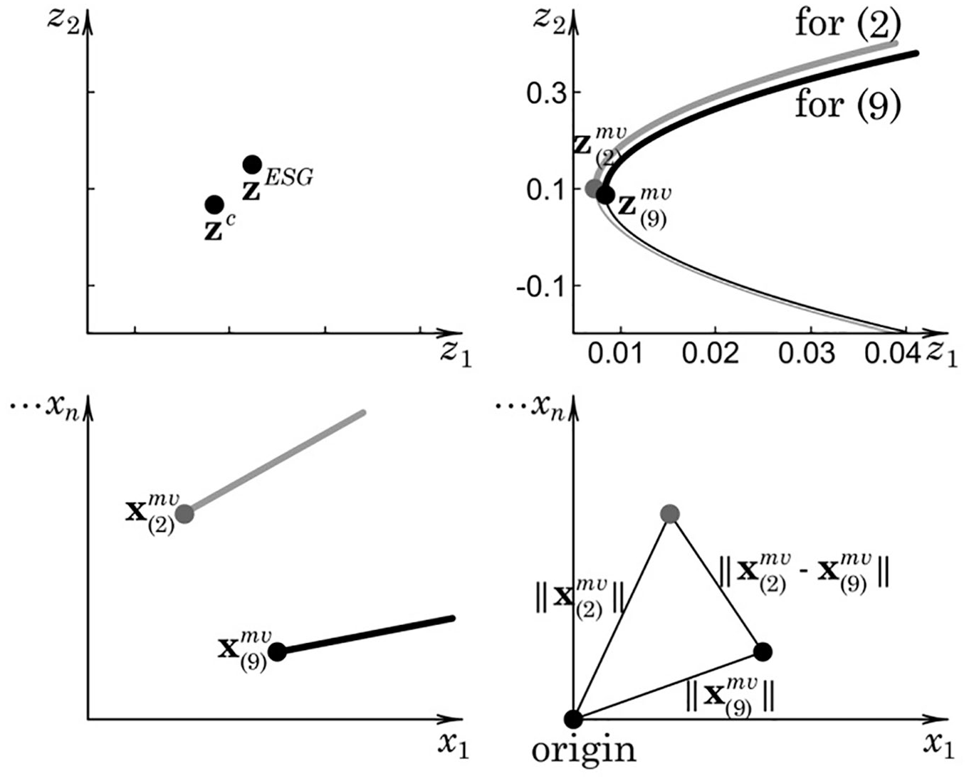
2. We then compute the optimal solutions of our model as a thick black curve in the upper right part of Figure 1. We also depict the optimal solutions of the conventional model as a thick gray curve in the upper right part. Therefore, we compare the two curves instead of basically focusing on only z^ESG and z^c in the upper left part.

3. Fundamentally, we compute the thick black curve’s portfolio weights as a black ray in the weight space in the lower left part of Figure 1. We also compute the thick gray curve’s portfolio weights as a gray ray. Therefore, we compare the two rays. Specifically, we quantitatively compare the rays’ apexes in the lower right part (i.e., ${\mathbf{x}}_{\left(2\right)}^{mv}$ vs. ${\mathbf{x}}_{\left(9\right)}^{mv}$ ).

We sample the component stocks of Dow Jones Industrial Average Index from 2004 to 2013. We find that the thick black curve and thick gray curve are similar but the black ray and gray ray are totally different. The practical implication is that sustainable investors can still obtain risk-return performance similar to that of conventional portfolio selection after imposing strong ESG requirements although the portfolio weights can be totally different from those of conventional portfolio selection. The result is both an endorsement and a reminder for sustainable investment. Endorsement means that sustainable investors can obtain risk-return performance similar to that of conventional investors even after imposing ESG constraints. Reminder means that sustainable investors should mind the highly different portfolio weights.

Overall, our aim is comparing the portfolio weights of sustainable portfolio selection and of conventional portfolio selection; the comparison result has been unknown until now. The result is important for sustainable investment because portfolio weights are the foundation of portfolio selection and investments. Our comparison methodology is portfolio-selection models of Markowitz (1959). No other scholars have conducted the comparison before. Therefore, our methodology is exploratory and based on modeling instead of testing hypotheses.

The rest of this article is organized as follows: We review portfolio selection and portfolio optimization in the next section. We briefly compare major methods of portfolio optimization in the next section. We impose ESG constraints and construct portfolio-selection models for sustainable investment in the next section. Computationally, we calculate the minimum-variance frontier in the next section. We then calculate the efficient frontiers of our model and conventional models in the weight space in the next section. We illustrate the analysis by an example in the next section. We conclude this article in the next section. We put proofs in the appendix.

Portfolio Selection and Portfolio Optimization

Portfolio Selection

Markowitz (1959) emphasizes that “Two objectives, however, are common to all investors . . . 1. They want ‘return’ to be high . . . 2. They want this return to be dependable” (p. 6). Then, for “a balanced whole,” he formulates portfolio selection by two-objective optimization as follows:

$$\begin{array}{l}\min \{z_1={\mathbf{x}}^T\Sigma \mathbf{x}\}\\ \max \{z_2={\mu }^T\mathbf{x}\}\\ \mathrm{s}.\mathrm{t}.\mathbf{x}\in S,\end{array}$$

(1)

where for n stocks, µ is a vector of stock expected-returns, Σ is a covariance matrix of stock returns, and superscript T denotes transposition. ⁵ Brockwell and Davis (1987) define covariance matrices as symmetric and positive semidefinite. Moreover, x is a portfolio-weight vector; z₁ and z₂, respectively, measure the variance and expectation of the return of portfolio x. Furthermore, $\mathrm{S}\subset {ℝ}^n$ is a feasible region; $\mathrm{Z}=\{(z_1,z_2)|\mathbf{x}\in \mathrm{S}\}$ is the feasible region in $(z_1,z_2)$ space.

Markowitz (1959) calls the optimal solutions of Equation 1 as an efficient frontier. For example, the efficient frontier is depicted as a thick gray curve in the upper right part of Figure 1.

Markowitz (1959) then suggests “first, separates efficient from inefficient portfolios; second, portrays . . . efficient portfolios; third, . . . select the combination . . . that best suits his needs; and fourth, determines the portfolio” (p. 7). He computes (whole) efficient frontiers and then asks investors to pinpoint their preferred portfolios from the frontiers, so investors never worry about missing some parts of the frontiers. Therefore, computing (whole) efficient frontiers is important for his suggestions.

Portfolio Optimization

Sharpe (1970) and Merton (1972) study the following model:

$$\begin{array}{l}\min \{z_1={\mathbf{x}}^T\Sigma \mathbf{x}\}\\ \max \{z_2={\mu }^T\mathbf{x}\}\\ \mathrm{s}.\mathrm{t}.1^T\mathbf{x}=1,\end{array}$$

(2)

where 1 is a vector of ones. Merton (1972) analytically solves the model; “analytical” means in the form of formulae. Equation 2 is a fundamental model of portfolio selection and thus described in classic finance textbooks (e.g., those of Bodie et al., 2018; Campbell, 2018; and Huang and Litzenberger, 1988). Moreover, Equation 2 serves as a basis of capital asset pricing models.

Merton (1972) applies an ϵ—constraint method (as described by Steuer, 1986) to Equation 2 as follows:

$$\begin{array}{l}\min \{z_1={\mathbf{x}}^T\Sigma \mathbf{x}\}\\ \mathrm{s}.\mathrm{t}.{\mu }^T\mathbf{x}=ϵ\\ 1^T\mathbf{x}=1,\end{array}$$

(3)

where ϵ is the parameter. The ${[z_1{z}_2]}^T$ set of all optimal solutions of Equation 3 with varying ϵ is called minimum-variance frontier of Equation 2. The frontier is the boundary of the feasible region Z of Equation 2. Merton (1972) analytically computes the frontier and proves it as a parabola as follows:

$$z_1=\frac{1}{af-c^2}\left(f{z}_2^2-2c{z}_2+a\right),$$

(4)

where symbols a, c, and f are introduced as follows:

$$a={\mathbf{\mu }}^T{\Sigma }^{-1}\mathrm{\mu },c=1^T{\Sigma }^{-1}\mathrm{\mu },f=1^T{\Sigma }^{-1}1.$$

(5)

The minimum-variance frontier of Equation 4 is depicted as a gray curve in the upper right part of Figure 1. The efficient frontier is the minimum-variance frontier’s upper portion and depicted as a thick gray curve. Merton (1972) computes the minimum-variance portfolio of Equation 2 (i.e., the optimal solution of $\min \left\{{\mathbf{x}}^T\Sigma \mathbf{x}\right\}$ , s.t. $1^T\mathbf{x}=1$ ) as follows:

$${\mathbf{x}}_{\left(2\right)}^{mv}=\frac{1}{f}{\Sigma }^{-1}1.$$

(6)

Merton (1972) computes the x set of the efficient frontier of Equation 2 as:

$${\mathrm{E}}_{\left(2\right)}=\left\{\mathbf{x}\in {ℝ}^n|\mathbf{x}=\lambda {\mathbf{j}}_{\left(2\right)}+{\mathbf{x}}_{\left(2\right)}^{mv},\lambda \in \left[0,\infty \right)\right\},$$

(7)

where

$${\mathbf{j}}_{\left(2\right)}=\frac{1}{2}\left({\Sigma }^{-1}\mu -\frac{c}{f}{\Sigma }^{-1}1\right).$$

(8)

The set is a ray; that is, the ray is generated by ${\mathbf{j}}_{\left(2\right)}$ and then translated to ${\mathbf{x}}_{\left(2\right)}^{mv}$ . The ray is depicted in the lower left part of Figure 1.

Comparing Major Portfolio-Optimization Methods

We briefly compare major portfolio-optimization methods and depict the result, advantage, and disadvantage in Figure 2.

Figure 2.

The result, advantage, and disadvantage of major portfolio-optimization methods.

Analytical Methods

Analytical methods are based on calculus and linear algebra and thus understandable. Merton (1972) analytically solves Equation 2 and obtains complete optimal solution information. For example, the minimum-variance frontier $z_1=0.350z_2^2-0.070z_2+0.011$ is depicted as a parabola in the first part of Figure 2. The efficient frontier is the upper portion and depicted as a thick curve. Qi et al. (2017) and Qi and Steuer (2020) extend Equation 2 and analytically solve multiple-objective portfolio selection. Analytical methods’ unique advantage is to readily compute the minimum-variance frontier including the efficient frontier.

However, analytical methods are for models with equality constraints only. Unpractically unbounded portfolio weights are thus allowed. Nevertheless, with almost all results in formulae, analytical methods bypass the need of mathematical programming and bring convenience in research and instruction. Huang and Litzenberger (1988) emphasize Equation 2 as “popular because of its analytical tractability and its rich empirical implications” (p. 60).

Parametric Quadratic Programming

Markowitz and Todd (2000) deploy parametric quadratic programming and propose a critical-line algorithm to solve Equation 1. Markowitz and Todd (2000) prove that the efficient frontier is piece-wisely made up by connected parabolic segments. For example, the frontier consists of two segments in the second part of Figure 2. The segment between ${\mathbf{z}}^1$ and ${\mathbf{z}}^2$ is a portion of parabola $z_1=3z_2^2-z_2+3;$ the segment between ${\mathbf{z}}^2$ and ${\mathbf{z}}^3$ is a portion of parabola $z_1=9z_2^2-z_2+9$ . Best (1996), Stein et al. (2008), and Hirschberger et al. (2010) also suggest their parametric quadratic programming algorithms. However, parametric quadratic programming is difficult to understand and thus rarely utilized.

Repetitive Quadratic Programming

Repetitive quadratic programming can be formulated as Equation 3. A group of ϵ is preset. Equation 2 is then repetitively solved for each ϵ; the optimal solutions are obtained for approximating the efficient frontier.

Repetitive quadratic programming is easier to understand than parametric quadratic programming and thus described in classic textbooks (e.g., those of Bodie et al., 2018; Elton et al., 2014; and Best, 2010). However, repetitive quadratic programming obtains only incomplete information of efficient frontiers by discrete approximations and thus cannot reveal the frontier structure. In the third part of Figure 2, the gray curve is copied from the second part as a comparison; repetitive quadratic programming obtains three points: ${\mathbf{z}}^4$ , ${\mathbf{z}}^5$ , and ${\mathbf{z}}^6$ . The gray curve is insufficiently approximated by the points.

Heuristic Methods

Some models with additional nonlinear formulation are difficult to solve; heuristic methods thus become important provisional tools. Evolutionary algorithms, tabu search, and simulated annealing can be common approaches (as reported by Woodside-Oriakhi et al., 2011).

However, heuristic methods inherently provide suboptimal solutions and only incomplete information of efficient frontiers and cannot reveal the frontier structure. In the fourth part of Figure 2, the methods obtain three points ${\mathbf{z}}^7,$ ${\mathbf{z}}^8$ , and ${\mathbf{z}}^9$ . Three broken lines demonstrate the difference between suboptimal solutions and optimal solutions.

Imposing ESG Constraints and Constructing Portfolio-Selection Models for Sustainable Investment

We extend Equation 2, explicitly impose ESG as constraints, and obtain the following general model:

$$\begin{array}{l}\min \{z_1={\mathbf{x}}^T\Sigma \mathbf{x}\}\\ \max \{z_2={\mu }^T\mathbf{x}\}\\ \mathrm{s}.\mathrm{t}.1^T\mathbf{x}=1,\end{array}$$

(9)

$$\begin{array}{l}{\mathbf{e}}^T\mathbf{x}=e\\ {\mathbf{s}}^T\mathbf{x}=s\\ {\mathbf{g}}^T\mathbf{x}=g\\ ⋮\end{array}$$

(10)

where e, s, and g are vectors of expected ESG of the stocks, respectively. e, s, and g are expected environmental, social, and governance of the portfolio, respectively. Symbol ⋮ denotes other constraints (e.g., thematic exposure) in Equation 10.

We introduce the following symbols:

$$\mathbf{A}\equiv {\left[\begin{array}{c}{1}^T\\ {\mathbf{e}}^T\\ {\mathbf{s}}^T\\ {\mathbf{g}}^T\\ ⋮\end{array}\right]}_{m\times n}\mathbf{b}\equiv {\left[\begin{array}{c}1\\ e\\ s\\ g\\ ⋮\end{array}\right]}_{m\times 1}.$$

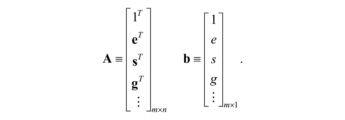
We then rewrite Equation 9 in matrix format as follows:

$$\begin{array}{l}\min \{z_1={\mathbf{x}}^T\Sigma \mathbf{x}\}\\ \max \{z_1={\mu }^T\mathbf{x}\}\\ \mathrm{s}.\mathrm{t}.\mathbf{A}x=\mathbf{b}.\end{array}$$

(11)

We inherit the assumptions of Merton (1972) and extend them as follows:

• Assumption 1.

• As a covariance matrix, Σ is invertible and thus positive definite.

• Assumption 2.

• Vector μ and all row vectors of A (altogether $m+1$ vectors) are linearly independent.

The assumptions are not strict prerequisite because of the following:

• By index models in finance (e.g., Bodie et al., 2018, Chapter 8), we obtain $\Sigma =\beta \Omega {\beta }^T+\mathbf{D}$ where for n stocks and i indexes, β is an $n\times i$ coefficient matrix, Ω is an $i\times i$ covariance matrix of the i indexes, and D is an $n\times n$ diagonal matrix with positive diagonal elements. With $\beta \Omega {\beta }^T$ as positive semidefinite and D as positive definite, Σ is positive definite.

• If the $m+1$ vectors are dependent, some vectors are linearly combined and the corresponding objective function or constraints can be consequently deleted.

With the vectors for Equation 9 as n-vectors, we know $(m+1)\le n$ by Assumption 2.

Analytically Deriving the Minimum-Variance Frontier of Equation 9

We follow Merton (1972) and also apply an ϵ-constraint method to Equation 11 and obtain

$$\begin{array}{l}\min \{z_1=x^T\Sigma \mathbf{x}\}\\ s.\mathrm{t}.{\mu }^{T}x=ϵ\\ \mathbf{A}x=\mathbf{b},\end{array}$$

(12)

where ϵ is the parameter. The application’s financial interpretation is taking ϵ as a target expected portfolio return and minimizing portfolio variance with ${\mu }^{T}x=ϵ$ and $\mathbf{A}x=\mathbf{b}.$ The set of ${[\begin{array}{cc}{z}_1& z_2\end{array}]}^T$ vectors of all optimal solutions of Equation 12 with varying ϵ is the minimum-variance frontier of Equation 9 and is an extension of the minimum-variance frontier of Equation 2. We introduce the following symbols:

$$\mathbf{H}\equiv {\left[\begin{array}{c}{\mu }^T\\ \mathbf{A}\end{array}\right]}_{\left(m+1\right)\times n}\mathbf{f}\equiv {\left[\begin{array}{c}ϵ\\ \mathbf{b}\end{array}\right]}_{\left(m+1\right)\times 1}.$$

(13)

We then rewrite all constraints of Equation 12 as $\mathbf{H}x=\mathbf{f}$ . The system of linear equations $\mathbf{H}x=\mathbf{f}$ is always solvable by Assumption 2. To solve Equation 12, we apply a Lagrange-multiplier method and construct:

$$\mathrm{L}\left(\mathbf{x},\ell \right)={\mathbf{x}}^T\Sigma \mathbf{x}+{\ell }^T\left(\mathbf{H}x-\mathbf{f}\right),$$

where $\ell$ is an $(m+1)$ —Lagrange-multiplier vector. Because $\mathrm{L}(\mathbf{x},\ell )$ is a convex function with respect to x by Assumption 1, x is the optimal solution of Equation 12 if and only if:

$$\begin{array}{l}\frac{\partial \mathrm{L}}{\partial \mathbf{x}}=2\Sigma \mathbf{x}+{\mathbf{H}}^T\ell =0\\ \frac{\partial \mathrm{L}}{\partial \ell }=\mathbf{H}x-\mathbf{f}=0,\end{array}$$

We premultiply the first partial-derivative equation by ${\Sigma }^{-1}$ and obtain

$$\mathbf{x}=-\frac{1}{2}{\Sigma }^{-1}{\mathbf{H}}^T\ell .$$

We then substitute x into the second partial-derivative equation and obtain

$$\left(\mathbf{H}{\Sigma }^{-1}{\mathbf{H}}^T\right)\ell =-2\mathbf{f}.$$

We propose the following lemma about the invertibility of ${(\mathbf{H}{\Sigma }^{-1}{\mathbf{H}}^T)}_{\left(m+1\right)\times \left(m+1\right)}$ for later computations:

• Lemma 1.

• Matrix $(\mathbf{H}{\Sigma }^{-1}{\mathbf{H}}^T)$ is a covariance matrix and positive definite and thus invertible.

Then, we premultiply $(\mathbf{H}{\Sigma }^{-1}{\mathbf{H}}^T)\ell =-2\mathbf{f}$ by ${(\mathbf{H}{\Sigma }^{-1}{\mathbf{H}}^T)}^{-1}$ and obtain $\ell =-2{(\mathbf{H}{\Sigma }^{-1}{\mathbf{H}}^T)}^{-1}\mathbf{f}$ . We substitute $\ell$ into $\mathbf{x}=-\frac{1}{2}{\Sigma }^{-1}{\mathbf{H}}^T\ell$ and obtain the optimal solution of Equation 12 as:

$$\mathbf{x}={\Sigma }^{-1}{\mathbf{H}}^T{(\mathbf{H}{\Sigma }^{-1}{\mathbf{H}}^T)}^{-1}\mathbf{f}.$$

We substitute x into $z_1={\mathbf{x}}^T\Sigma \mathbf{x}$ of Equation 9 and compute the minimum-variance frontier as:

$$\begin{array}{c}{z}_1=({\Sigma }^{-1}{{\mathbf{H}}^T(\mathbf{H}{\Sigma }^{-1}{\mathbf{H}}^T)}^{-1}\mathbf{f})T\Sigma ({\Sigma }^{-1}{\mathbf{H}}^T\left(\mathbf{H}{\Sigma }^{-1}{\mathbf{H}}^T{)}^{-1}\mathbf{f}\right)\\ =({\mathbf{f}}^T\left(\mathbf{H}{\Sigma }^{-1}{\mathbf{H}}^T{)}^{-1}\mathbf{H}{\Sigma }^{-1}\right)\Sigma ({\Sigma }^{-1}{\mathbf{H}}^T\left(\mathbf{H}{\Sigma }^{-1}{\mathbf{H}}^T{)}^{-1}\mathbf{f}\right)\\ ={\mathbf{f}}^T{(\mathbf{H}{\Sigma }^{-1}{\mathbf{H}}^T)}^{-1}\left(\mathbf{H}{\Sigma }^{-1}{\mathbf{H}}^T\right){(\mathbf{H}{\Sigma }^{-1}{\mathbf{H}}^T)}^{-1}\mathbf{f}\\ ={\mathbf{f}}^T{(\mathbf{H}{\Sigma }^{-1}{\mathbf{H}}^T)}^{-1}\mathbf{f},\end{array}$$

We use symbols $z_2$ instead of ϵ of Equation 13 to present the frontier in (z₁, z₂) space of Equation 9 as:

$$z_1=\left[\begin{array}{cc}{z}_2& {\mathbf{b}}^T\end{array}\right]{(\mathbf{H}{\Sigma }^{-1}{\mathbf{H}}^T)}^{-1}\left[\begin{array}{c}{z}_2\\ \mathbf{b}\end{array}\right].$$

(14)

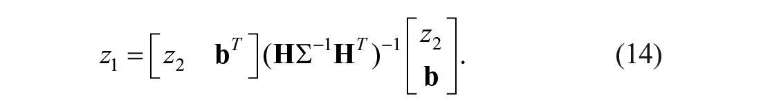
The minimum-variance frontier of Equation 14 is more complicated than Equation 2. Moreover, we prove the frontier also as a parabola in the following theorem:

• Theorem 1.

• The minimum-variance frontier of Equation 14 is a parabola in (z₁, z₂) space of Equation 9.

By Theorem 1 and Equation 12, the parabola of Equation 14 is the boundary of the feasible region Z of Equation 9. Moreover, the efficient frontier of Equation 9 is the parabola’s upper portion. We have already depicted the parabola as a black curve in the upper right part of Figure 1.

Analytically Deriving the Efficient Frontier of Equation 9

We follow Sharpe (1970) and also apply a weighted-sums method (as described by Steuer, 1986) to Equation 11 and obtain:

$$\begin{array}{l}\min \left\{{\mathbf{x}}^T\Sigma \mathbf{x}-\lambda {\mu }^T\mathbf{x}\right\}\\ \mathrm{s}.\mathrm{t}.\mathbf{A}x=\mathbf{b},\end{array}$$

(15)

where λ is the parameter. The application’s financial interpretation is taking λ as a risk-aversion parameter, computing the expected utility (i.e., $-{\mathbf{x}}^T\Sigma \mathbf{x}+\lambda {\mu }^T\mathbf{x}$ ), and maximizing the expected utility. We then apply a Lagrange-multiplier method to Equation 15 and construct:

$$\mathrm{L}\left(\mathbf{x},\ell \right)={\mathbf{x}}^T\Sigma \mathbf{x}-\lambda {\mu }^T\mathbf{x}+{\ell }^T\left(\mathbf{A}x-\mathbf{b}\right),$$

where $\ell$ is an m—Lagrange-multiplier vector. For notation-consistency reasons, we still utilize symbols $\mathrm{L}(\mathbf{x},\ell )$ and $\ell$ , but they are different from those in the previous section. Because $\mathrm{L}(\mathbf{x},\ell )$ is a convex function with respect to x by Assumption 1, x is the optimal solution of Equation 15 if and only if:

$$\begin{array}{l}\frac{\partial \mathrm{L}}{\partial \mathbf{x}}=2\Sigma \mathbf{x}-\lambda \mu +{\mathbf{A}}^T\ell =0\\ \frac{\partial \mathrm{L}}{\partial \ell }=\mathbf{A}x-\mathbf{b}=0.\end{array}$$

We premultiply the first partial-derivative equation by ${\Sigma }^{-1}$ and obtain:

$$\mathbf{x}=\frac{1}{2}{\Sigma }^{-1}\left(\lambda \mu -{\mathbf{A}}^T\ell \right).$$

We substitute x into the second partial-derivative equation and obtain:

$$\mathbf{A}\frac{1}{2}{\Sigma }^{-1}\left(\lambda \mu -{\mathbf{A}}^T\ell \right)-\mathbf{b}=0,$$

and rearrange it as

$$\begin{array}{l}\mathbf{A}{\Sigma }^{-1}\lambda \mu -\left(\mathbf{A}{\Sigma }^{-1}{\mathbf{A}}^T\right)\ell -2\mathbf{b}=0\\ \left(\mathbf{A}{\Sigma }^{-1}{\mathbf{A}}^T\right)\ell =\mathbf{A}{\Sigma }^{-1}\lambda \mu -2\mathbf{b}.\end{array}$$

We know $(\mathbf{A}{\Sigma }^{-1}{\mathbf{A}}^T)$ as invertible by the proof of Lemma 1 and premultiply the equation above by ${(\mathbf{A}{\Sigma }^{-1}{\mathbf{A}}^T)}^{-1}$ . We then obtain:

$$\ell ={(\mathbf{A}{\Sigma }^{-1}{\mathbf{A}}^T)}^{-1}\left(\mathbf{A}{\Sigma }^{-1}\lambda \mu -2\mathbf{b}\right),$$

and substitute $\ell$ into $\mathbf{x}=(1/2){\Sigma }^{-1}(\lambda \mu -{\mathbf{A}}^T\ell )$ as:

$$\begin{array}{c}\mathbf{x}=\frac{1}{2}{\Sigma }^{-1}(\lambda \mu -{\mathbf{A}}^T\left(\mathbf{A}{\Sigma }^{-1}{\mathbf{A}}^T{)}^{-1}\left(\mathbf{A}{\Sigma }^{-1}\lambda \mu -2\mathbf{b}\right)\right)\\ =\frac{1}{2}{\Sigma }^{-1}\lambda \mu -\frac{1}{2}{\Sigma }^{-1}{\mathbf{A}}^T{(\mathbf{A}{\Sigma }^{-1}{\mathbf{A}}^T)}^{-1}\left(\mathbf{A}{\Sigma }^{-1}\lambda \mu \right)+\\ {\Sigma }^{-1}{\mathbf{A}}^T{(\mathbf{A}{\Sigma }^{-1}{\mathbf{A}}^T)}^{-1}\mathbf{b}\\ =\frac{1}{2}{\Sigma }^{-1}{\mathbf{I}}_{\mathrm{n}}\left(\lambda \mu \right)-\frac{1}{2}{\Sigma }^{-1}{\mathbf{A}}^T{(\mathbf{A}{\Sigma }^{-1}{\mathbf{A}}^T)}^{-1}\mathbf{A}{\Sigma }^{-1}\left(\lambda \mu \right)+\\ {\Sigma }^{-1}{\mathbf{A}}^T{(\mathbf{A}{\Sigma }^{-1}{\mathbf{A}}^T)}^{-1}\mathbf{b},\end{array}$$

where ${\mathbf{I}}_{\mathrm{n}}$ is an $n\times n$ identity matrix. The optimal solution of Equation 15 is:

$$\begin{array}{l}\mathbf{x}=\frac{\lambda }{2}{\Sigma }^{-1}({\mathbf{I}}_{\mathrm{n}}-{\mathbf{A}}^T\left(\mathbf{A}{\Sigma }^{-1}{\mathbf{A}}^T{)}^{-1}\mathbf{A}{\Sigma }^{-1}\right)\mu +\\ {\Sigma }^{-1}{\mathbf{A}}^T{(\mathbf{A}{\Sigma }^{-1}{\mathbf{A}}^T)}^{-1}\mathbf{b}.\end{array}$$

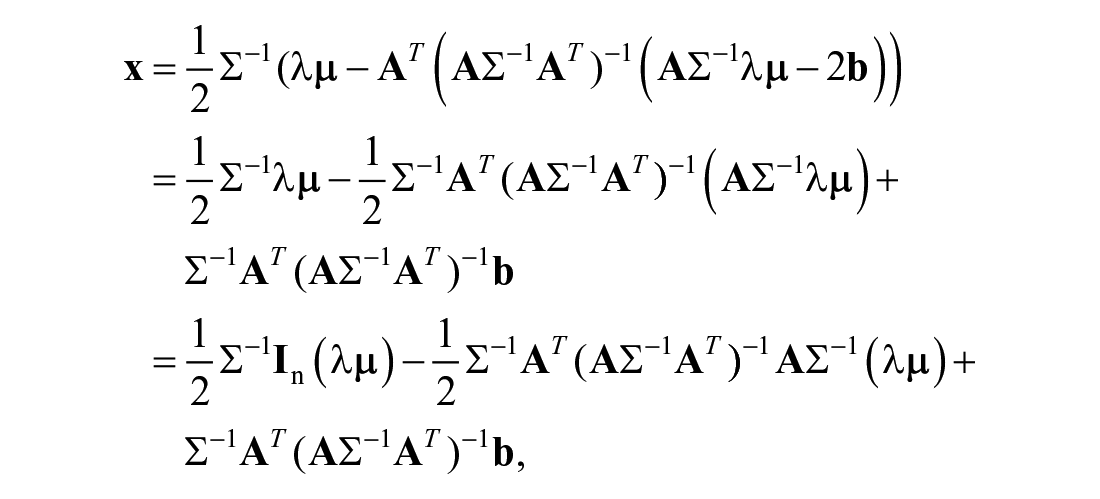
To demonstrate the x set’s properties, we introduce an $n\times 1$ symbol as follows:

$${\mathbf{j}}_{\left(9\right)}\equiv \frac{1}{2}{\Sigma }^{-1}({\mathbf{I}}_{\mathrm{n}}-{\mathbf{A}}^T\left(\mathbf{A}{\Sigma }^{-1}{\mathbf{A}}^T{)}^{-1}\mathbf{A}{\Sigma }^{-1}\right)\mu \mathrm{.}$$

(16)

where subscript (9) is for Equation 9. We then rewrite the optimal solution as:

$$\mathbf{x}=〈/b〉\lambda {\mathbf{j}}_{\left(9\right)}+{\mathbf{x}}_{\left(9\right)}^{mv},$$

(17)

$${\mathbf{x}}_{\left(9\right)}^{mv}=\Sigma {\mathbf{A}}^T{(\mathbf{A}{\Sigma }^{-1}{\mathbf{A}}^T)}^{-1}\mathbf{b},$$

(18)

where ${\mathbf{x}}_{\left(9\right)}^{mv}$ is the minimum-variance portfolio of Equation 9 with $\lambda =0$ for Equation 15; that is, ${\mathbf{x}}_{\left(9\right)}^{mv}$ is the optimal solution of $\min \left\{{\mathbf{x}}^T\Sigma \mathbf{x}\right\},\mathrm{s}.\mathrm{t}.\mathbf{A}x=\mathbf{b}$ . On the basis of Equation 17, we summarize the result in the following theorem:

• Theorem 2.

• The $〈/i〉\mathbf{x}$ set of the efficient frontiers of Equation 9 is:

$$E_{\left(9\right)}=\{\mathbf{x}\in {ℝ}^n|\mathbf{x}=\lambda {\mathbf{j}}_{\left(9\right)}+{\mathbf{x}}_{\left(9\right)}^{mv},\lambda \in \left[0,\infty \right)\}.$$

(19)

The set is a ray; that is, the ray is generated by $j_{\left(9\right)}$ and then translated to ${\mathbf{x}}_{\left(9\right)}^{mv}$ .

We have already depicted the ray in the lower left part of Figure 1.

Comparing the Efficient Frontiers of Equations 2 and 9 in the Weight Space

We have already computed the x sets of Equations 7 and 19 of the efficient frontiers of Equations 2 and 9. We also have demonstrated Equations 7 and 19 as rays. By the ray structure, we compare the x sets:

• Comparing ${\mathbf{x}}_{\left(2\right)}^{mv}$ and ${\mathbf{x}}_{\left(9\right)}^{mv}$ .

We compare ${\mathbf{x}}_{\left(2\right)}^{mv}$ and ${\mathbf{x}}_{\left(9\right)}^{mv}$ by proposing a changing ratio as follows:

$$\delta =\frac{\parallel {\mathbf{x}}_{\left(2\right)}^{mv}-{\mathbf{x}}_{\left(9\right)}^{mv}\parallel }{\parallel {\mathbf{x}}_{\left(2\right)}^{mv}\parallel +\parallel {\mathbf{x}}_{\left(9\right)}^{mv}\parallel },$$

(20)

where $\parallel \parallel$ denotes lengths by $l^2$ -norm. We have already depicted the ratio in the lower right part of Figure 1. Because $\parallel {\mathbf{x}}_{\left(2\right)}^{mv}\parallel +\parallel {\mathbf{x}}_{\left(9\right)}^{mv}\parallel \ge \parallel {\mathbf{x}}_{\left(2\right)}^{\mathrm{mv}}-{\mathbf{x}}_{\left(9\right)}^{mv}\parallel$ , we obtain $0\le \delta \le 1$ .

• If ${\mathbf{x}}_{\left(2\right)}^{mv}$ and ${\mathbf{x}}_{\left(9\right)}^{mv}$ completely overlap (i.e., ${\mathbf{x}}_{\left(2\right)}^{mv}={\mathbf{x}}_{\left(9\right)}^{mv}$ ), we obtain $\delta =0$ .

• If ${\mathbf{x}}_{\left(2\right)}^{mv}$ and ${\mathbf{x}}_{\left(9\right)}^{mv}$ are completely opposite (i.e., ${\mathbf{x}}_{\left(2\right)}^{mv}=-{\mathbf{x}}_{\left(9\right)}^{mv}$ ), we obtain $\delta =1$ .

Comparing the x Sets

Although ${\mathbf{x}}_{\left(2\right)}^{mv}$ of Equation 6 is simpler than ${\mathbf{x}}_{\left(9\right)}^{mv}$ of Equation 18, and although ${\mathbf{j}}_{\left(2\right)}$ of Equation 8 is simpler than ${\mathbf{j}}_{\left(9\right)}$ of Equations 16, 2, and 9, they have similar efficient frontier structure (i.e., rays of Equations 7 and 19). By the ray structure, we prove that portfolio selection for sustainable investment and conventional portfolio selection fundamentally possess highly different portfolio-weight vectors in the following theorem:

• Theorem 3.

• For the relationship between the x sets of the efficient frontiers of Equations 2 and 9, there are three exhaustive and exclusive cases: complete overlap, only one intersection, and no intersection.

Complete-overlap case requires ${\mathbf{x}}_{\left(2\right)}={\mathbf{x}}_{\left(9\right)}$ and ${\mathbf{j}}_{\left(2\right)}={\mathbf{j}}_{\left(9\right)}.$ It is relatively easy to detect the case by comparing Equation 6 against Equation 18 and comparing Equation 8 against Equation 16.

We then compare the two x sets by basically checking whether they intersect. If they intersect, they have one identical portfolio-weight vector. Otherwise, they have completely different portfolio-weight vectors (i.e., no similarity). By the ray structure, we formulate the intersection as follows:

$${\lambda }_{\left(2\right)}{\mathbf{j}}_{\left(2\right)}+{\mathbf{x}}_{\left(2\right)}^{mv}={\lambda }_{\left(9\right)}{\mathbf{j}}_{\left(9\right)}+{\mathbf{x}}_{\left(9\right)}^{mv},{\lambda }_{\left(2\right)}\ge 0,{\lambda }_{\left(9\right)}\ge 0.$$

(21)

We rearrange Equation 21 into the following linear-equation-system format:

$$\begin{array}{l}{\lambda }_{\left(2\right)}{\mathbf{j}}_{\left(2\right)}-{\lambda }_{\left(9\right)}{\mathbf{j}}_{\left(9\right)}={\mathbf{x}}_{\left(9\right)}^{mv}-{\mathbf{x}}_{\left(2\right)}^{mv}\\ {\left[\begin{array}{cc}{\mathbf{j}}_{\left(2\right)}& -{\mathbf{j}}_{\left(9\right)}\end{array}\right]}_{n\times 2}{\left[\begin{array}{c}{\lambda }_{\left(2\right)}\\ {\lambda }_{\left(9\right)}\end{array}\right]}_{2\times 1}=({\mathbf{x}}_{\left(9\right)}^{mv}-{\mathbf{x}}_{\left(2\right)}^{mv})n\times 1\end{array}$$

(22)

where ${\lambda }_{\left(2\right)}$ and ${\lambda }_{\left(9\right)}$ are the unknowns. We construct the augmented matrix for Equation 22 as follows:

$$\mathbf{J}\equiv {\left[\begin{array}{ccc}{\mathbf{j}}_{\left(2\right)}& -{\mathbf{j}}_{\left(9\right)}& |\left({\mathbf{x}}_{\left(9\right)}^{mv}-{\mathbf{x}}_{\left(2\right)}^{mv}\right)\end{array}\right]}_{n\times 3}.$$

We propose the following theorem for the intersection possibility under three exhaustive and exclusive situations:

• Theorem 4.

• If $rank〈/i〉([\begin{array}{cc}{j}_{\left(2\right)}& -j_{\left(9\right)}\end{array}])=rank\left(\mathbf{J}\right)$ , Equation 22 is solvable. Moreover, if there exist ${\lambda }_{\left(2\right)}\ge 0$ and ${\lambda }_{\left(9\right)}\ge 0$ , the x sets of the efficient frontiers of Equations 2 and 9 intersect.

• If $rank([\begin{array}{cc}{j}_{\left(2\right)}& -j_{\left(9\right)}\end{array}])=rank\left(\mathbf{J}\right)$ but there do not exist ${\lambda }_{\left(2\right)}\ge 0$ and ${\lambda }_{\left(9\right)}\ge 0$ , the x sets of the efficient frontiers of Equations 2 and 9 do not intersect.

• If $rank([\begin{array}{cc}{j}_{\left(2\right)}& -j_{\left(9\right)}\end{array}])\ne rank\left(\mathbf{J}\right)$ , Equation 22 is insolvable. Therefore, the x sets of the efficient frontiers of Equations 2 and 9 do not intersect.

An Illustration

We utilize the following model on the basis of Equation 9:

$$\begin{array}{l}\min \{z_1={\mathbf{x}}^T\Sigma \mathbf{x}\}\\ \max \{z_2={\mu }^T\mathbf{x}\}\\ \mathrm{s}.\mathrm{t}.1^T\mathbf{x}=1\\ {\mathbf{e}}^T\mathbf{x}=e\\ {\mathbf{s}}^T\mathbf{x}=s\\ {\mathbf{g}}^T\mathbf{x}=g.\end{array}$$

Measuring ESG

Carroll (2000) argues for the reason and method to theoretically measure corporate social responsibility (CSR) which typically subsumes ESG. In practice, there are several professional organizations to measure ESG or more broadly measure CSR, for example, RobecoSAM AG, Sustainalytics, the KLD Research & Analytics (KLD), ARESE, and Thomson Reuters ESG data.

On one side, Hopkins (2005) criticizes the measurement systems by demonstrating several indicators as subjectively chosen. Entine (2003) draws similar conclusions. On the other side, Waddock and Graves (1997) review CSR-measure problems and conclude KLD as relatively reliable. Kang (2015), Hart and Sharfman (2015), and Waddock (2003) draw similar conclusions. Overall, Mattingly and Berman (2006), Chatterji et al. (2009), and Hart and Sharfman (2015) relatively comprehensively evaluate KLD ratings. Turker (2009) realizes the measurement methods’ limitation and proposes a new method on the basis of stakeholders’ responsibility. Graafland et al. (2004) utilize similar methods.

KLD adopts the following categories: alcohol, community, corporate governance, diversity, employee relations, environment, firearms, gambling, human rights, military, nuclear power, product, and tobacco. KLD typically divides a category into two subcategories: strengths and concerns, but some categories (e.g., alcohol) have only concerns. KLD then constructs binary variables under all subcategories. Therefore, a category measurement can be computed by adding all the strengths variables under the category and then subtracting all the concerns variables under the category. Specifically,

• For environmental of ESG, the category environment can be utilized.

• For social of ESG, the summation of categories community, diversity, employee relations, human rights, and product can be utilized.

• For governance of ESG, the category corporate governance can be utilized.

Dyck et al. (2019), Halbritter and Dorfleitner (2015), and Galema et al. (2009) utilize similar methods.

Sampling

For Equation 9, we select the following 27 component stocks of Dow Jones Industrial Average Index because they have complete observations whereas the other component stocks do not: Apple (AAPL), American Express (AXP), Boeing (BA), Caterpillar (CAT), Cisco (CSCO), Chevron (CVX), Disney (DIS), Dow Chemical (DOW), Goldman Sachs (GS), Home Depot (HD), IBM (IBM), Intel (INTC), Johnson & Johnson (JNJ), JPMorgan Chase (JPM), Coca-Cola (KO), McDonald’s (MCD), 3M (MMM), Merck (MRK), Microsoft (MSFT), Nike (NKE), Pfizer (PFE), Procter & Gamble (PG), United Health (UNH), United Technologies (UTX), Verizon (VZ), Wal-Mart (WMT), and Exxon Mobil (XOM). (data source: https://us.spindices.com/indices/equity/dow-jones-industrial-average, S&P Dow Jones Indices LLC., October 22, 2019). To save space, we list just brief company names with ticker symbols above.

The sample is made up of the 27 stocks’ monthly return and annual ESG data from January 1, 2004, to December 31, 2013 (data source: database “CRSP” and database “MSCI ESG KLD STATS” via Wharton Research Data Services, https://wrds-web.wharton.upenn.edu/wrds/, October 24, 2019). When we wrote this article, the latest data of “MSCI ESG KLD STATS” was for 2016. However, the ESG data from 2014 to 2016 have many missing values. Therefore, we sample from 2004 to 2013.

We compute the sample covariance matrix and sample mean vector of the stocks’ return and then assume the sample statistics as the population parameters (i.e., Σ and μ, respectively) because Elton et al. (2014) contend that “It is common to use historical risk, return, and correlation as a starting point in obtaining inputs for calculating the efficient frontier” (p. 87). We annualize Σ and μ by the method of Bodie et al. (2018) and report them in Table 1.

Table 1.

The Σ and μ of the 27 Component Stocks of Equation 9.

Σ	AAPL	AXP	BA	CAT	CSCO	CVX	DIS	DOW	GS	HD	IBM	INTC	JNJ	JPM	KO	MCD	MMM	MRK	MSFT	NKE	PFE	PG	UNH	UTX	VZ	WMT	XOM
AAPL	.134	.051	.028	.044	.032	.030	.029	.058	.049	.016	.025	.042	.008	.020	.009	.020	.022	.009	.037	.023	.001	.011	.023	.022	.014	−.001	.022
AXP	.051	.142	.050	.073	.048	.019	.049	.137	.049	.036	.024	.037	.017	.061	.014	.012	.043	.010	.038	.036	.018	.019	.033	.039	.017	.009	.012
BA	.028	.050	.064	.035	.030	.019	.032	.060	.027	.017	.012	.025	.015	.030	.010	.010	.025	.023	.019	.020	.020	.010	.028	.031	.014	.003	.015
CAT	.044	.073	.035	.119	.048	.035	.042	.094	.054	.033	.027	.039	.012	.045	.018	.018	.040	.011	.032	.035	.023	.019	.025	.040	.022	.010	.024
CSCO	.032	.048	.030	.048	.078	.018	.031	.058	.040	.031	.027	.040	.010	.034	.010	.008	.027	.013	.030	.027	.013	.014	.016	.027	.011	.005	.011
CVX	.030	.019	.019	.035	.018	.037	.018	.026	.018	.009	.011	.014	.007	.011	.009	.012	.017	.009	.016	.010	.012	.007	.010	.015	.015	.002	.027
DIS	.029	.049	.032	.042	.031	.018	.050	.064	.031	.021	.019	.026	.013	.031	.014	.013	.023	.015	.022	.024	.016	.011	.021	.025	.013	.009	.012
DOW	.058	.137	.060	.094	.058	.026	.064	.193	.065	.041	.030	.042	.017	.075	.015	.010	.051	.013	.043	.051	.022	.022	.042	.049	.017	.012	.016
GS	.049	.049	.027	.054	.040	.018	.031	.065	.099	.018	.026	.029	.012	.055	.014	.013	.019	.014	.035	.025	.011	.009	.015	.030	.015	.011	.015
HD	.016	.036	.017	.033	.031	.009	.021	.041	.018	.049	.015	.020	.006	.031	.005	.005	.019	.002	.019	.017	.012	.006	.014	.015	.010	.013	.003
IBM	.025	.024	.012	.027	.027	.011	.019	.030	.026	.015	.034	.022	.008	.020	.007	.009	.014	.007	.012	.012	.004	.006	.015	.015	.006	.005	.008
INTC	.042	.037	.025	.039	.040	.014	.026	.042	.029	.020	.022	.065	.014	.022	.012	.012	.021	.021	.029	.024	.012	.009	.018	.023	.012	.009	.010
JNJ	.008	.017	.015	.012	.010	.007	.013	.017	.012	.006	.008	.014	.019	.014	.011	.008	.011	.016	.010	.008	.012	.011	.013	.012	.008	.006	.006
JPM	.020	.061	.030	.045	.034	.011	.031	.075	.055	.031	.020	.022	.014	.087	.013	.011	.023	.013	.027	.028	.025	.015	.021	.032	.008	.013	.009
KO	.009	.014	.010	.018	.010	.009	.014	.015	.014	.005	.007	.012	.011	.013	.025	.010	.010	.015	.013	.012	.013	.010	.002	.007	.012	.006	.008
MCD	.020	.012	.010	.018	.008	.012	.013	.010	.013	.005	.009	.012	.008	.011	.010	.024	.005	.011	.013	.012	.010	.010	.010	.010	.010	.005	.011
MMM	.022	.043	.025	.040	.027	.017	.023	.051	.019	.019	.014	.021	.011	.023	.010	.005	.039	.007	.013	.018	.010	.011	.011	.021	.009	.005	.009
MRK	.009	.010	.023	.011	.013	.009	.015	.013	.014	.002	.007	.021	.016	.013	.015	.011	.007	.061	.016	.003	.025	.010	.024	.017	.014	.005	.011
MSFT	.037	.038	.019	.032	.030	.016	.022	.043	.035	.019	.012	.029	.010	.027	.013	.013	.013	.016	.055	.019	.011	.009	.012	.018	.018	.006	.011
NKE	.023	.036	.020	.035	.027	.010	.024	.051	.025	.017	.012	.024	.008	.028	.012	.012	.018	.003	.019	.050	.009	.011	.009	.017	.007	.008	.002
PFE	.001	.018	.020	.023	.013	.012	.016	.022	.011	.012	.004	.012	.012	.025	.013	.010	.010	.025	.011	.009	.039	.014	.021	.017	.013	.006	.012
PG	.011	.019	.010	.019	.014	.007	.011	.022	.009	.006	.006	.009	.011	.015	.010	.010	.011	.010	.009	.011	.014	.022	.012	.012	.007	.003	.007
UNH	.023	.033	.028	.025	.016	.010	.021	.042	.015	.014	.015	.018	.013	.021	.002	.010	.011	.024	.012	.009	.021	.012	.075	.024	.009	.000	.010
UTX	.022	.039	.031	.040	.027	.015	.025	.049	.030	.015	.015	.023	.012	.032	.007	.010	.021	.017	.018	.017	.017	.012	.024	.035	.011	.004	.011
VZ	.014	.017	.014	.022	.011	.015	.013	.017	.015	.010	.006	.012	.008	.008	.012	.010	.009	.014	.018	.007	.013	.007	.009	.011	.038	.009	.012
WMT	−.001	.009	.003	.010	.005	.002	.009	.012	.011	.013	.005	.009	.006	.013	.006	.005	.005	.005	.006	.008	.006	.003	.000	.004	.009	.024	.000
XOM	.022	.012	.015	.024	.011	.027	.012	.016	.015	.003	.008	.010	.006	.009	.008	.011	.009	.011	.011	.002	.012	.007	.010	.011	.012	.000	.031
(μ)T	.474	.149	.173	.174	.037	.158	.158	.128	.119	.133	.104	.038	.096	.117	.089	.177	.095	.081	.095	.199	.046	.086	.141	.127	.130	.071	.129

Note. AAPL = Apple; AXP = American Express; BA = Boeing; CAT = Caterpillar; CSCO = Cisco; CVX = Chevron; DIS = Disney; DOW = Dow Chemical; GS = Goldman Sachs; HD = Home Depot; IBM = IBM Company; INTC = Intel; JNJ = Johnson & Johnson; JPM = JPMorgan Chase; KO = Coca-Cola; MCD = McDonald’s; MMM = 3M; MRK = Merck; MSFT = Microsoft; NKE = Nike; PFE = Pfizer; PG = Procter & Gamble; UNH = United Health; UTX = United Technologies; VZ = Verizon; WMT = Wal-Mart; XOM = Exxon Mobil.

For example, the covariance between AAPL and AXP is .051 in the second row. The expected return of AAPL is .474 in the last row.

We adopt the ESG measurement for KLD, compute ESG from 2004 to 2013, and report them in Table 2. For example, the ESG of AAPL in 2004 is 0, 1, and −1, respectively. Moreover, we compute the sample mean vectors of the ESG and then assume the sample statistics as the population parameters (i.e., e, s, and g, respectively). We also report e, s, and g in Table 2. For example, the expected ESG of AAPL are 1.2, −0.2, and −0.8, respectively.

Table 2.

The e, s, and g of the 27 Component Stocks of Equation 9.

	AAPL	AXP	BA	CAT	CSCO	CVX	DIS	DOW	GS	HD	IBM	INTC	JNJ	JPM	KO	MCD	MMM	MRK	MSFT	NKE	PFE	PG	UNH	UTX	VZ	WMT	XOM
2004	0	0	−2	0	0	−4	1	−1	0	1	−2	1	0	0	−1	1	−1	−2	0	1	−1	0	0	1	−1	−1	−5
2005	1	0	−2	−1	1	−4	1	−1	0	1	1	2	2	0	0	0	0	−3	0	3	0	−1	0	0	−1	−1	−5
2006	1	0	−2	−1	1	−4	1	−1	0	1	2	2	1	0	1	0	1	−1	0	3	0	−1	0	1	0	−1	−5
2007	1	0	−2	−1	1	−3	1	−1	0	0	2	2	2	0	1	0	1	−1	0	3	1	0	0	0	0	−1	−4
2008	1	0	−4	0	1	−3	1	−1	0	1	2	2	2	0	2	1	0	−1	0	3	1	0	0	1	0	−1	−4
2009	1	0	−4	0	1	−3	1	−1	0	1	2	2	2	0	2	1	0	−1	0	3	1	0	0	1	0	−1	−4
2010	3	2	1	1	4	−3	3	0	2	0	3	4	4	2	0	1	2	1	3	3	3	2	1	1	2	1	−1
2011	3	2	0	1	4	−3	4	0	4	1	4	4	4	4	0	1	3	2	3	3	3	3	1	2	2	0	−1
2012	0	1	0	1	3	0	1	1	1	0	2	5	3	1	0	0	4	1	2	2	3	4	0	2	1	0	−2
2013	1	1	4	1	2	−3	1	2	1	1	5	5	4	0	0	1	2	4	4	2	1	5	0	4	2	2	−1
(e)T	1.2	0.6	−1.1	0.1	1.8	−3	1.5	−0.3	0.8	0.7	2.1	2.9	2.4	0.7	0.5	0.6	1.2	−0.1	1.2	2.6	1.2	1.2	0.2	1.3	0.5	−0.3	−3.2
2004	1	3	1	−2	7	1	0	2	3	−3	7	9	5	3	−3	1	6	3	6	4	4	6	2	2	5	−4	−1
2005	1	8	3	−2	6	0	0	−1	3	−2	9	7	6	2	0	1	6	4	4	5	4	7	0	−1	3	−5	−2
2006	0	8	4	−2	6	−1	−1	−1	3	−1	11	9	6	2	0	0	6	3	4	3	3	7	0	0	3	−6	−2
2007	0	8	4	−3	6	−1	−1	2	2	−1	12	12	5	2	0	−1	4	3	5	3	1	6	−1	0	2	−5	−3
2008	−1	8	2	−3	6	−1	−2	2	1	−1	11	11	6	1	0	0	3	3	5	5	0	6	0	−3	2	−5	−4
2009	−1	8	2	−4	6	−2	−2	2	1	−1	11	11	6	1	0	0	3	3	5	5	−1	6	0	−3	2	−5	−4
2010	−2	5	−2	−2	7	4	0	1	−1	1	8	13	10	1	1	3	−1	10	5	4	3	11	2	−1	3	−1	−1
2011	0	6	1	0	7	6	3	3	0	5	10	14	10	1	6	4	2	11	7	8	3	12	4	0	4	0	0
2012	−1	7	6	6	8	4	8	−1	5	4	6	11	4	4	3	2	4	5	6	7	3	6	1	2	3	−2	5
2013	1	7	8	4	10	7	5	3	7	6	7	12	3	5	8	−1	4	8	8	6	0	5	5	2	4	−3	4
(s)T	−0.2	6.8	2.9	−0.8	6.9	1.7	1	1.2	2.4	0.7	9.2	10.9	6.1	2.2	1.5	0.9	3.7	5.3	5.5	5	2	7.2	1.3	−0.2	3.1	−3.6	−0.8
2004	−1	−1	−1	−1	−1	0	−1	0	−2	−1	−1	0	−2	−2	−1	0	−1	−1	−1	0	−1	−1	−2	−1	−1	−1	−1
2005	0	−1	0	−1	0	0	−1	1	−1	−1	−1	1	0	−1	−2	2	0	−3	1	0	0	1	−1	−1	0	−1	−2
2006	−1	−1	−2	−1	−1	−1	−2	−1	−2	−1	−2	0	0	−2	−3	1	0	−1	1	1	0	0	−2	0	−1	−3	−3
2007	−1	−1	−2	−1	−1	−1	−2	0	−2	−4	−2	1	1	−2	−2	1	0	−2	2	2	−1	0	−2	0	−1	−3	−2
2008	−1	−1	−2	−2	−1	−1	−2	−1	−2	−4	−2	1	0	−2	−2	1	0	−1	2	2	0	0	−2	0	−1	−3	−2
2009	−1	−1	−2	−2	−1	−1	−2	−1	−2	−4	−2	1	0	−2	−2	1	0	−1	2	2	0	0	−2	0	−1	−3	−2
2010	−1	0	−2	0	1	0	1	1	−1	−3	−1	0	1	−1	0	−1	1	0	0	2	0	0	−1	0	0	−1	−1
2011	−1	1	−1	0	1	0	1	2	−1	−1	0	1	1	−1	0	−1	1	0	1	2	0	1	−1	0	1	−1	−1
2012	0	0	2	0	0	0	0	0	−3	−1	0	0	−1	−3	0	−1	2	0	2	0	1	−1	−1	1	2	0	1
2013	−1	0	0	−1	−1	−1	0	0	0	0	0	0	−2	−3	0	0	1	0	1	0	0	−1	−1	−1	0	−1	1
(g)T	−0.8	−0.5	−1	−0.9	−0.4	−0.5	−0.8	0.1	−1.6	−2	−1.1	0.5	−0.2	−1.9	−1.2	0.3	0.4	−0.9	1.1	1.1	−0.1	−0.1	−1.5	−0.2	−0.2	−1.7	−1.2

Note. AAPL = Apple; AXP = American Express; BA = Boeing; CAT = Caterpillar; CSCO = Cisco; CVX = Chevron; DIS = Disney; DOW = Dow Chemical; GS = Goldman Sachs; HD = Home Depot; IBM = IBM Company; INTC = Intel; JNJ = Johnson & Johnson; JPM = JPMorgan Chase; KO = Coca-Cola; MCD = McDonald’s; MMM = 3M; MRK = Merck; MSFT = Microsoft; NKE = Nike; PFE = Pfizer; PG = Procter & Gamble; UNH = United Health; UTX = United Technologies; VZ = Verizon; WMT = Wal-Mart; XOM = Exxon Mobil.

For Equation 9, we take:

$$\begin{array}{l}e=\mathrm{the}75\mathrm{th}\mathrm{percentile}\mathrm{of}\mathbf{e}=1.275\\ s=\mathrm{the}75\mathrm{th}\mathrm{percentile}\mathrm{of}\mathbf{s}=5.450\\ g=\mathrm{the}75\mathrm{th}\mathrm{percentile}\mathrm{of}\mathbf{g}=-0.100.\end{array}$$

Solving Equation 9

By Equation 14, we compute the minimum-variance frontier of Equation 9 as follows:

$$\begin{array}{c}{z}_1={\left[\begin{array}{c}{z}_2\\ 1\\ 1.275\\ 5.450\\ -0.100\end{array}\right]}^T\\ \left[\begin{array}{ccccc}.387& -.039& -.003& .002& .004\\ -.039& .013& .000& .000& .001\\ -.003& .000& .001& .000& -.001\\ .002& .000& .000& .000& .000\\ .004& .001& -.001& .000& .002\end{array}\right]\left[\begin{array}{c}{z}_2\\ 1\\ 1.275\\ 5.450\\ -0.100\end{array}\right]\\ =0.387z_2^2-0.069z_2+0.011.\end{array}$$

We have already plotted the frontier as a black parabola in Figure 1. The frontier’s upper half is the efficient frontier of (29) and is plotted as a thick curve.

We compute ${\mathbf{j}}_{\left(9\right)}$ by Equation 16, compute ${\mathbf{x}}_{\left(9\right)}^{mv}$ by Equation 18, and report them in Table 3. We substitute ${\mathbf{x}}_{\left(9\right)}^{mv}$ into Equation 9 to obtain the minimum-variance portfolio in $\left(z_1,z_2\right)$ space as follows:

Table 3.

${\mathbf{j}}_{\left(9\right)}$ j₍₉₎ of Equation 16 and (x ^mv ₍₉₎) of Equation 18.

	AAPL	AXP	BA	CAT	CSCO	CVX	DIS	DOW	GS	HD	IBM	INTC	JNJ	JPM	KO	MCD	MMM	MRK	MSFT	NKE	PFE	PG	UNH	UTX	VZ	WMT	XOM
(j(9)) T	1.70	0.23	0.79	0.70	−0.78	0.79	0.33	−0.75	−0.71	0.60	0.05	−1.45	1.08	0.75	−1.51	0.74	−0.79	1.01	−0.69	1.81	−1.54	−0.09	−0.24	−0.64	0.74	−1.40	−0.73
(x mv (9)) T	−0.03	0.02	−0.02	−0.13	−0.05	0.01	−0.05	−0.06	0.02	0.05	0.23	0.00	0.12	−0.08	−0.02	0.02	0.14	−0.02	0.08	0.14	0.06	0.24	0.00	0.06	0.04	0.12	0.11

Note. AAPL = Apple; AXP = American Express; BA = Boeing; CAT = Caterpillar; CSCO = Cisco; CVX = Chevron; DIS = Disney; DOW = Dow Chemical; GS = Goldman Sachs; HD = Home Depot; IBM = IBM Company; INTC = Intel; JNJ = Johnson & Johnson; JPM = JPMorgan Chase; KO = Coca-Cola; MCD = McDonald’s; MMM = 3M; MRK = Merck; MSFT = Microsoft; NKE = Nike; PFE = Pfizer; PG = Procter & Gamble; UNH = United Health; UTX = United Technologies; VZ = Verizon; WMT = Wal-Mart; XOM = Exxon Mobil.

$${\mathbf{z}}_{\left(9\right)}^{mv}={\left[\begin{array}{cc}0.008& 0.089\end{array}\right]}^T.$$

We then compute $E_{\left(9\right)}$ by Equation 19.

Solving Equation 2

As a comparison, we also solve Equation 2 for the 27 component stocks. By Equation 2, we compute the minimum-variance frontier of Equation 2 as follows:

$$z_1=0.350z_2^2-0.070z_2+0.011.$$

We compute ${\mathbf{j}}_{\left(2\right)}$ by Equation 8, compute ${\mathbf{x}}_{\left(2\right)}^{mv}$ by Equation 6, and report them in Table 4. We substitute ${\mathbf{x}}_{\left(2\right)}^{mv}$ into Equation 2 to obtain the minimum-variance portfolio in $\left(z_1,z_2\right)$ space as follows:

Table 4.

${\mathbf{j}}_{\left(2\right)}$ j₍₂₎ of Equation 8 and (x ^mv ₍₂₎) of Equation 6.

	AAPL	AXP	BA	CAT	CSCO	CVX	DIS	DOW	GS	HD	IBM	INTC	JNJ	JPM	KO	MCD	MMM	MRK	MSFT	NKE	PFE	PG	UNH	UTX	VZ	WMT	XOM
(j(2)) T	2.14	0.01	0.53	0.92	−0.51	−0.12	0.60	−0.73	−0.82	0.83	−0.54	−1.96	1.19	0.75	−0.57	0.81	−0.99	0.76	−1.02	1.54	−1.49	−1.11	−0.07	0.41	0.61	−0.71	−0.44
(x mv (2)) T	−0.01	0.01	−0.01	−0.12	−0.03	0.00	−0.06	−0.04	0.01	0.08	0.13	−0.05	0.02	−0.08	0.10	0.03	0.10	−0.02	0.05	0.09	0.01	0.17	0.04	0.15	0.00	0.24	0.18

Note. AAPL = Apple; AXP = American Express; BA = Boeing; CAT = Caterpillar; CSCO = Cisco; CVX = Chevron; DIS = Disney; DOW = Dow Chemical; GS = Goldman Sachs; HD = Home Depot; IBM = IBM Company; INTC = Intel; JNJ = Johnson & Johnson; JPM = JPMorgan Chase; KO = Coca-Cola; MCD = McDonald’s; MMM = 3M; MRK = Merck; MSFT = Microsoft; NKE = Nike; PFE = Pfizer; PG = Procter & Gamble; UNH = United Health; UTX = United Technologies; VZ = Verizon; WMT = Wal-Mart; XOM = Exxon Mobil.

$${\mathbf{z}}_{\left(2\right)}^{mv}={\left[\begin{array}{cc}0.007& 0.100\end{array}\right]}^T.$$

We then compute $E_{\left(2\right)}$ by Equation 7.

Comparing the x Sets of the Efficient Frontiers of Equations 9 and 2

By Equation 20, we compute $\delta =0.287$ . For Equation 22, we compute $rank([\begin{array}{cc}{\mathbf{j}}_{\left(2\right)}& -{\mathbf{j}}_{\left(9\right)}\end{array}])=2$ and $rank\left(\mathbf{J}\right)=3$ . Therefore, by Theorem 4, the x sets of the efficient frontiers of Equations 9 and 2 do not intersect.

Changing e, s, and g to the 50th Percentiles and 90th Percentiles

In addition to the 75th percentile setting for e, s, and g, we also reset them as the 50th percentiles and then reset them as the 90th percentiles. We depict the minimum-variance frontiers (including the efficient frontiers) for the 50th percentiles, 75th percentiles, and 90th percentiles in the upper left, upper right, and lower parts of Figure 3, respectively. Overall, the results of the 50th and 90th percentiles are similar to those of the 75th percentiles.

Figure 3.

The results of setting e, s, and g as the 50th, 75th, and 90th percentiles for Equation 9.

Conclusion and Future Direction

Researching sustainable investment is challenging; difficulties in extending conventional portfolio selection are encountered in this article. However, the researching is worthwhile because sustainable investment will no longer be practical experience and will become a theoretically and quantitatively robust tool for investment on the basis of portfolio selection.