Sage Journals: Discover world-class research

Abstract

This article examines the influence of relative prices, production capacity, gross domestic product, fish export and trawl fishing bans, and seasonality on Oman’s fish exports to the European Union (EU), Southeast-, East- and South Asia (SEA), and the Gulf Cooperation Council (GCC) markets during 2001–2015. Following the prescribed “keep it sensibly simple” rule for practitioners and the lack of any empirical evidence to support better alternatives, a partial adjustment framework is used to describe the dynamics of fish export behavior. The appropriate functional form was decided by testing the nested Cobb–Douglas (CD) hypothesis within the constant elasticity of substitution (CES) specification and the result supports the CD specification. The models were estimated using ordinary least square (OLS). The descriptive statistical results indicate market heterogeneity in species preferences. The empirical results suggest some degree of inertia in adjustment in the EU and SEA markets. The negative impact of the “export ban” on the EU market suggests a “trade-off” between the protection of domestic consumers and the revenue forgone. The export is price elastic in the short-run for the EU market. The impact of the “trawl fishing ban” on the EU and GCC markets was negative and positive, respectively. The significance of “production capacity” for the GCC and SEA markets signals that future enhancement strategies of exports should be aligned with the long-term sustainability of fish resources. The error-correction model could be considered to check the robustness of the present findings. An examination of the sensitivity of export-supply to potential risks should also be useful.

Keywords

seafood export export ban trawl fishing ban partial adjustment model Oman

Introduction

The fisheries sector plays an important socio-economic role in terms of food and nutrition security, employment, income and foreign exchange earnings in Oman (Al-Busaidi et al., 2016; Al-Subhi et al., 2013; FSB, 2000–2016). Recently, this sector has been identified as one of the five (that includes manufacturing, logistic services, tourism, and mining) promising sectors in the ninth 5-year plan (2016–2020). One of the key strategic objectives stipulated in the ninth 5-year plan (2016–2020) is to enhance the development of the seafood industries and to promote the export of value-added products and the quality of Omani seafood products, in the domestic and global markets (Ministry of Agriculture and Fisheries [MAF], 2015).

Oman is a net exporter of seafood products (Al-Busaidi et al., 2016; Al-Subhi et al., 2013; Bose et al., 2010). The sector’s reliance on export earnings is evident by the fact that in 2016, 54% of the total landings (280,000 metric tons [mt]) were exported. The total fish landings increased from 120,000 mt in 2000 to 280,000 mt in 2016, while the total seafood exports increased from 46,000 mt in 2000 to 152,000 mt in 2016. The gross value of total landings increased from 53 million Omani Rial (OMR; 1 OMR = US$2.59) in 2000 to 204 million OMR in 2016, while the gross value of fish exports increased from 37 million OMR in 2000 to 73 million OMR in 2016 (FSB, 2000–2016).

The seafood processing companies mainly supply fresh and frozen products of locally caught species (grouped to into five categories, namely, large pelagic, small pelagic, demersal, sharks and rays, and crustaceans and molluscs) to domestic, regional, and international markets. During the 2000 to 2016 period, the major export destinations for Oman’s seafood products were the Gulf Cooperation Council (GCC) countries, countries belonging to the Southeast-, East-, and South Asia (SEA), and the European Union (EU) countries. According to 2017 estimates, about 38 seafood processing firms with the Hazard Analysis and Critical Control Point (HACCP) system target major international markets (such as the EU, the United States, and Japan) with strict quality and safety standards. On the contrary, about 20 processers without the HACCP system target less-stringent markets such as the GCC, the SEA, and so on (Al-Busaidi et al., 2016; MAF, 2018).

Recently, Bose et al. (2019) noted that the performance of seafood exports measured in terms of quantity and value in the EU market has deteriorated during the past years (see Figure 1). This type of decline in export to high-value markets such as the EU has important economic implications for the sector as it has a negative impact on foreign exchange earnings. In addition, since 2011, the MAF has implemented export bans with various rates (20%–100%) under different Ministerial Decisions (MDs). The demand for such government intervention was influenced by the lack of availability of preferred fish and high fish prices in the domestic market. Therefore, the application of this quantitative export restraint measures was decided by the government to protect domestic consumers’ interests and ensure availability of these preferred species in the domestic market and thereby to reduce inflationary pressure on fish prices (Bose et al., 2019). In 2011, the demersal trawl fishery stopped its operation due to a ban imposed on demersal trawl fishing. These types of regulatory measures may influence the export-supply to some markets as such restrictions may create competition between the domestic and foreign markets if species preferences are similar. It may also create a significant shift in demand in foreign markets.

Figure 1.

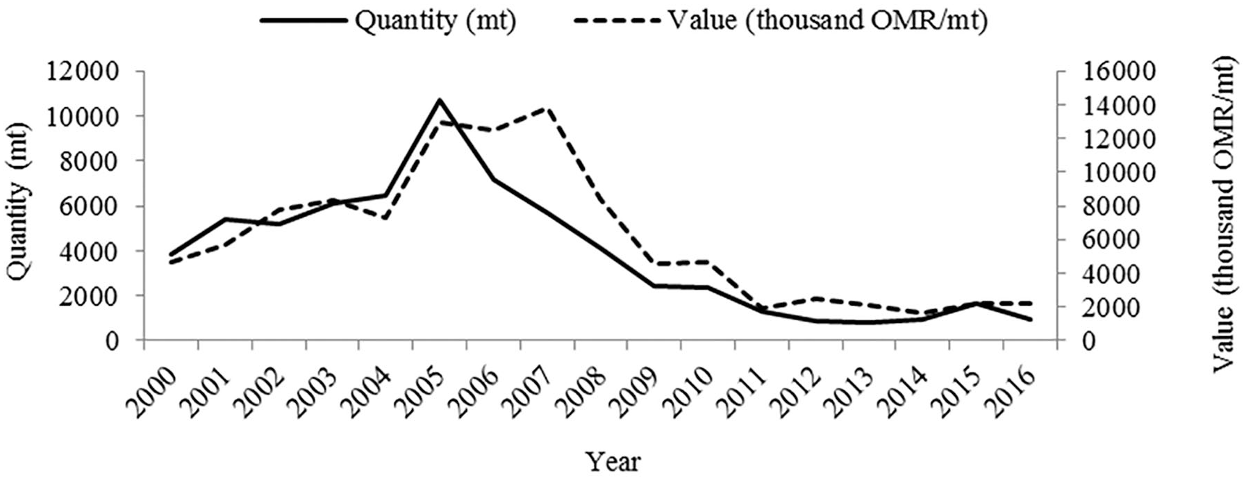
Quantity and value of seafood export to the EU market: 2000–2016.

Given this background, the main aim of this study is to empirically examine the effect of domestic regulatory measures (i.e., seafood export ban and trawl fishing ban), relative price, production capacity, gross domestic product, seasonality, and time trend on Oman’s seafood export-supply to three broadly grouped markets, namely, the EU, the SEA, and the GCC covering the period 2001–2015. With particular reference to the above-mentioned domestic measures, testing of statistical significance of the following two hypotheses is of particular interest as the title of the article alludes:

Hypothesis 1: The export ban that has been introduced in 2011 is expected to have a negative effect on fish exports.

Hypothesis 2: The demersal trawl fishing ban of 2009 is expected to exert significant influence on seafood exports.

While various country-specific studies have been conducted on export-supply of fish and seafood products to a single-market segment (Bose & Galvan, 2005; Bose & Redkar, 2004), to the best of authors’ knowledge, this study is first of its kind in Oman that encompasses export performance in three distinct market segments, and to this end, this article not only fills the existing knowledge gap in seafood market research but also complements the existing global literature by adding country-specific information. In addition, this study contributes to the practical realm as well, as it provides policy makers and seafood businesses of local and global origins with quantitative and up-to-date knowledge about export market behavior which has the potential to assist in designing effective strategic actions.

It is observed that Oman has been exporting fish products to a number of countries like the United Arab Emirates (UAE), the Kingdom of Saudi Arabia (KSA), Bangladesh, Thailand, and India. This further rationalizes the importance of market analysis to identify heterogeneity in market preferences and thereby enhance the knowledge of the relevant actors of local origin and enable them to formulate appropriate marketing strategies to accommodate the market dynamics of foreign origin.

The earlier mentioned policy actions (i.e., demersal trawl fishing ban and domestic ban on fish exports) may influence fish exports to the foreign markets due to competition from the domestic market and supply-side disturbances due to fishing ban. Therefore, information on policy measures in Oman would help importers such as the EU to design alternative strategies to reduce supply uncertainty concerning their domestic markets.

The remainder of the article is structured as follows. A brief review of relevant studies that covered the application of various alternative empirical approaches to agricultural supply response analysis and a justification for the use of a partial adjustment approach are included in “Brief Review of Relevant Studies” section. “Data Description” and “Empirical Model” sections describe the data and empirical approach used for analytical purposes, respectively. Results are detailed in “Results” section. Discussion of results, policy issues, and concluding remarks with possible extensions of the this article are provided in “Discussion,” “Policy Issues,” and “Concluding Remarks” sections, respectively.

Brief Review of Relevant Studies

Since the seminal work of Nerlove (1956, 1979), the partial adjustment model (PAM) has gained its popularity in empirical analysis of supply response of agricultural commodities (Diebold & Lamb, 1997), particularly field crops (Wickens & Greenfield, 1973). Based on microeconomic theory, Nerlove (1956) justified an empirical framework for interpreting farmers’ responses to prices by estimating the PAM with adaptive expectation. Colman (1983) argued that the Nerlovian PAM reflects the inertia in the dependent variable to adjust to the desired level, emanating from adjustment costs, technological constraints, and so on, and it incorporates dynamic elements to the model. Lawrence (1990) explicitly took into account such imperfect adjustment and the associated costs of adjustment in modeling Canadian export and import demand responsiveness at an aggregate level.

Askari and Cummings (1977) presented a comprehensive review of its country-specific application involving many agricultural crops. Recent application of the Nerlovian model can be found in De Menezes and Piketty (2012), Gosalamang et al. (2012), and Shoko et al. (2016), exemplifying the fact that the Nerlovian model is still popular in agricultural supply response analysis. However, the application of the Nerlovian PAM in dealing with export-supply response of fisheries products is relatively limited. The PAM framework was adopted by Bose and Redkar (2004) and Bose and Galvan (2005) in estimating import demand and export-supply behavior of Indian and New Zealand seafood products, respectively.

Recognizing the close relationship between adjustment lags and expectations, various extensions of PAM have been applied by researchers through alternative expectations formation mechanisms (Just, 1977; Shideed & White, 1989; Shonkwiler, 1982). Askari and Cummings (1977) documented a number of empirical studies that used the adaptive expectations in supply response analysis. On the contrary, Kennan (1979), Eckstein (1985), and Chambers and Lopez (1984) applied the rational expectations model of Muth (1961) in analyzing supply response in a PAM setting. A modified PAM was also used by La France and Burt (1983) by focusing on the stochastic components of the dynamic regression model in analyzing U.S. agricultural supply. Griffiths and Anderson (1978) also found some empirical support for an additive disturbance in the specification of agricultural supply function of wheat in southern New South Wales, Australia. However, Shideed and White (1989) stated that no particular specification for producers’ expectations formation can claim superiority to its counterpart specifications.

Eckstein (1985) presented a simple rational expectations equilibrium model to derive the dynamic agricultural supply function from an explicit optimization problem that was demonstrated to be observationally equivalent with the Nerlovian model, but it rejected the adaptive expectations formula assumed by the Nerlovian model. Estrella and Fuhrer (2002) demonstrated with empirical evidence that various macroeconomic models with rational expectations and optimizing behavior can lead to dynamic inconsistencies and are often seriously at odds with the data. They pointed out that the inclusion of expectations in models does not warrant their empirical suitability.

Furthermore, to avoid the restrictive dynamics with the Nerlovian model, the autoregressive distributed lag (ADL) model has been considered as an alternative approach to the PAM in supply response analysis (Mbaga & Coyle, 2003). Phlips (1974) showed that the distributed lag model based on geometric distribution is observationally equivalent to the PAM. Shideed and White (1989) pointed out that the distributed lag model suffers from theoretical and statistical limitations. For instance, a problem lies with the ADL approach in the determination of appropriate lag length and the potential loss of degrees of freedom if a large number of parameters are to be estimated. In addition, the covariates are likely to be highly correlated with their lagged series and consequently undermine the reliability of the estimates (Gujarati, 2003).

A second alternative approach to the PAM is the cointegration and error-correction model (ECM) developed by Engle and Granger (1987). This two-step procedure investigates the existence of nonspurious long-run equilibrium relationships (i.e., cointegrating relationships), in its first step and then detects the extent of short-run deviation from the long-run equilibrium path through the inclusion of an error-correction term in the second step. In analyzing agricultural supply response, the ECM is used by Hallam and Zanoli (1993), Gunawardana et al. (1995), Carone (1996), Thiele (2000), and Olubode-Awosola et al. (2006), to name a few. Hallam and Zanoli (1993) claimed that the ECM is a superior alternative to PAM on both theoretical and empirical grounds. It is evident that both the ECM and the PAM have dynamic elements, deal with adjustment costs, and are based on partial equilibrium framework (Nichell, 1985). The ECM can be considered as a generalized version of the simple PAM (Hendry & von Ungern-Sternberg, 1981, cited in Alogoskoufis & Smith, 1991) and a reparameterization of the general ADL model under the application of the “general to specific” methodology (Alogoskoufis & Smith, 1991). However, unlike the PAM, the adjustment mechanism is derived through the specification and minimization of a “loss function” (Nichell, 1985). The specification of such a “loss function” or “adjustment costs function” poses additional complexity to the adjustment process. In relation to the ECM formulation, the researcher is free to eliminate or restrict the differenced variables if necessary but cannot exclude the error-correction term from the model as it incorporates the long-run equilibrium solution of the model (Gilbert, 1986). Like the distributed lag model, the ECM also faces criticism in relation to the determination of appropriate lag length and the potential loss of degrees of freedom if a large number of parameters are to be estimated.

Another alternative approach such as linear programming was also used in estimating and comparing supply elasticities with a simple partial adjustment supply model (Shumway & Chang, 1977). However, its use is relatively less frequent as it is data-intensive and context-driven. While the agricultural supply response analysis has witnessed the application of various extensions of the PAM specification and alternative approaches as discussed above, no claim to uniqueness seems plausible.

The econometric approach to supply response analysis is subdivided into three categories: (a) two-stage procedures, (b) system approach, and (c) directly estimated single-commodity models (Colman, 1983). However, Colman (1983) noted that the majority of the supply response studies of agricultural commodities involve direct estimation of the supply function from time-series data in which the supply response is measured at an aggregate level.

Colman (1983) argued in favor of the single-commodity models because of their simplicity in terms of estimation, handling dynamic adjustments, and data requirements. Shoko et al. (2016) justified the suitability of PAM due to computational simplicity. King and Thomas (2006) argued that the PAM may not adequately reflect the supply response behavior of individual processing firms, although the model performs relatively well at the aggregate level.

The variation in fish stock due to environmental and biological conditions and variation in fishing effort due to increases in fishing costs seem to be the most commonly encountered events which influence export-supply of fish and seafood products (Prochaska, 1984). Such variations are most likely to contribute to a slower response by fishers. Therefore, it is reasonable to assume that fish exports do not instantaneously adjust to their long-run equilibrium path resulting from a change in any of the independent variables.

This article adopts the “directly estimated single-commodity model” in the standard PAM setting. This choice is influenced by the following reasons revealed from the above discussion: (a) the fish export-supply behavior exhibits inertia in adjustment to the desired level (Bose & Galvan, 2005), (b) computational simplicity (Colman, 1983), (c) data availability, (d) relatively better performance of the model with aggregate data (King & Thomas, 2006), and (e) the nature of the research questions to be addressed. Furthermore, following the KISS (i.e., “keep it sensibly simple”) rule recommended by Kennedy (2002) for applied economists, it is felt that the PAM is more appropriate for the case in hand. Also, the standard PAM places relatively less unrealistic demand on the data. Finally, the results from the model diagnostics do not show any sign of inappropriateness of the model. Also, no information could be found on the extent of the adjustment costs.

Data Description

Quarterly data covering the period 2001–2015 were used in this study to facilitate the examination of seasonality in export-supply. The sample period was influenced by the availability of consistent data from all countries involved. For GCC countries and some SEA countries, available data for GDP and CPI were annual. Following Abeysinghe and Rajaguru (2004) and Lahari et al. (2011), these annual data variables were converted into quarterly figures using Eviews 8.0. The CPI data for all countries included in the analysis were converted to the same base year 2010 (=100). The data for real GDP were measured at constant price (2010=100). The aggregated export price for each regional market was calculated as a sum of weighted average export prices of individual markets in the region using each country’s export share as weight.

Data for relevant variables are expressed in U.S. dollars. Data were obtained from various national, regional, and international sources. For instance, data for quantities of fish landings and export and the MDs of the seafood export ban and trawl fishing ban were collected from MAF. The CPI data for Oman were obtained from the National Centre for Statistics and Information (NCSI). The data (GDP and CPI) for 28 EU countries were collected from the Organization for Economic Cooperation and Development (OECD) database. The GDP and CPI data for the SEA countries were obtained from the International Monetary Fund (IMF), OECD, and the World Bank. The GDP and CPI data for the GCC countries were collected from the Gulf Cooperation Council Statistics Centre (GCC-Stat) and the Secretariat General of the Gulf Cooperation Council (GCC-SG) Statistics, respectively.

It is worth mentioning that the data for each group of countries were aggregated to analyze them as one market. This is simply due to a lack country-specific data for each region with the desired regular intervals for analysis. Therefore, the fish exports data to the EU countries, the GCC countries, and 10 major destination countries (i.e., Bangladesh, Thailand, India, China, Indonesia, Vietnam, Malaysia, Sri Lanka, Republic of South Korea, and Hong Kong) of the SEA were aggregated to portray each regional market. It was noted that the selected countries of the SEA market represented on average about 95% of Oman’s total fish exports to the region. This type of aggregation of countries based on geographical region is not uncommon in commodity exports analysis. For instance, in estimating demand and supply elasticities of commodity exports of developing countries, Bond (1987) categorized countries into five geographical regions to highlight the interregional differences in such estimates.

Empirical Model

Applied economists are generally faced with the difficult task of choosing a functional form that would best represent and explain the true unknown nature of a technological relationship between dependent and independent variables. In an attempt to decide between the Cobb–Douglas (CD) and the constant elasticity of substitution (CES)—the two extensively used functional specifications in applied research—for the present analysis, the likelihood ratio (LR) test $(LR = - 2 (L_{CD} - L_{CES}) ~ χ^{2} (1))$ was applied to the “nested hypothesis” that represented the former as a special case of the later. In addition, the statistical significance of the “correction factor” that represents the departure of the substitution parameter from zero in the CES specification was examined. For analytical simplicity and to ensure balanced comparison of parameter estimates, the approximation proposed by Kmenta (1967) to the CES function of two key economic covariates, namely, relative prices (RP) and market size (proxied by GDP) is adopted. An obvious advantage of this transformation around the elasticity of substitution equal to unity as pointed out by Kmenta (1967) is that the parameters can be directly estimated by using simple least square regression techniques as it is linear in parameters that represent the powers of ln(RP), ln(GDP), and their ratio.

Findings from this experiment are as follows. First, the likelihood ratio (LR) test results (i.e., 1.62, 2.44, and 2.03 for the EU, SEA and GCC models, respectively) for the nested hypothesis, which follows a $χ^{2}$ distribution with 1 degree of freedom, indicate that the CD specification is appropriate as these calculated values were less than the tabulated value of $χ^{2}$ with 1 degree of freedom (i.e., 3.84) at the 5% level. Second, the estimated coefficient of the “correction factor” that represents the departure of substitution parameter from zero was not statistically significant at the 5% level for all three cases. The estimates (t value) were −0.772 (−1.22), 0.622 (1.48), and 0.111 (1.37) for the EU, SEA and GCC, respectively. Third, a surprising change in parameter estimates of ln(RP) and ln(GDP) from the CES specification (about 10–15 times larger in absolute value compared with the CD specification) for the EU and SEA models may be an indication of functional misspecification. Fourth, the diagnostic test results for the EU and GCC models under both functional specifications did not exhibit any deviation from the basic classical regression properties (i.e., normality of residuals, absence of autocorrelation, and homoscedasticity). However, to satisfy the same properties, two dummy variables (for first quarters of 2003 and 2007) were added to both functional specifications for the SEA model to capture sharp changes in export-supply data. Last but not least, compared with the CD specification, for all the models under the CES specification, the small improvement in the R² value (in the range .005–.017) was observed. Considered together, these empirical results do present a coherent picture and favor the CD functional specification over the CES.

Based on the review of literature presented earlier and the findings in relation to the functional specification, this article used a CD-type functional form under a partial adjustment framework as follows. In setting up the empirical framework, no consideration is given to the import demand for fish products in the present study. This is because of the fact that Oman has been a net exporter of fish products as stated earlier and the proportion of imports has always been trivial relative to exports:

\begin{array}{l} Q_{t}^{Oman} = (ϕ A) Q_{t - 1}^{(1 - ϕ)} {(RP)}^{ϕ α_{1}} {(PC)}^{ϕ α_{2}} {(GDP)}^{ϕ α_{3}} \\ {(\exp)}^{\sum_{i = 1}^{2} ϕ β_{i} {PD}_{i}} {(\exp)}^{\sum_{i = 1}^{3} ϕ γ_{i} {SD}_{i}} {(\exp)}^{ϕ δ (T)} {(\exp)}^{μ_{t}} . \end{array}

(1)

Taking “log” on both sides, Equation 1 can be represented as follows:

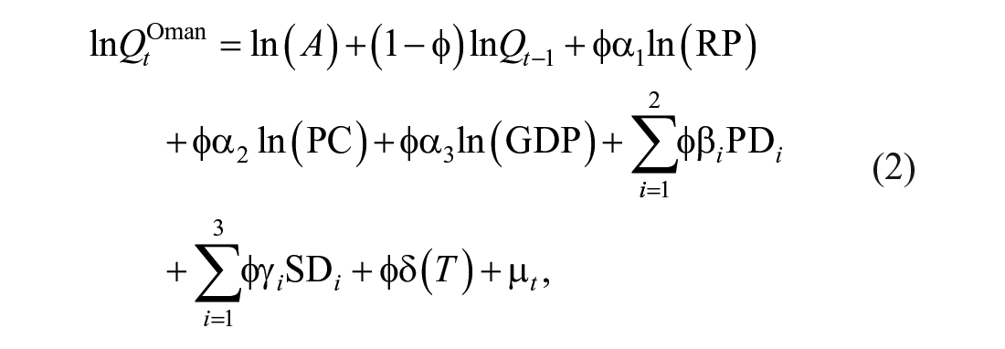
\begin{array}{l} \ln Q_{t}^{Oman} = \ln (A) + (1 - ϕ) \ln Q_{t - 1} + ϕ α_{1} \ln (RP) \\ + ϕ α_{2} \ln (PC) + ϕ α_{3} \ln (GDP) + \sum_{i = 1}^{2} ϕ β_{i} {PD}_{i} \\ + \sum_{i = 1}^{3} ϕ γ_{i} {SD}_{i} + ϕ δ (T) + μ_{t}, \end{array}

(2)

where the dependent variable $Q_{t}^{Oman}$ indicates the export-supply of seafood from Oman to each market, and “RP” represents relative price measured as the ratio of export price to domestic price. Domestic price was proxied by consumer price index (CPI) for seafood/food products, “PC” represents production capacity proxied by total fish landings (mt), GDP (gross domestic product) used as proxy for market size, and PD₁ and PD₂ are policy variables that represent the bans on seafood export of some species that came into effect in the second quarter of 2011 and on demersal trawl fishing that came into effect at the second quarter of 2009. The policy variable was measured as a dummy variable with the value “1” when the ban was enforced and “0” otherwise, seasonal dummy (SD) variables were used to capture the potential seasonality of export, and a trend variable (T) was used to estimate time-specific impacts such as changes in tastes and preferences, impact of technological change, and so on that might have a potential effect on Oman’s seafood supply over time. The symbols “α,” “β,” “γ,” and “δ” are coefficients to be estimated, “ϕ” is the adjustment parameter that represents the share of desired adjustment completed in a single period, and µ_t is the disturbance term. The average adjustment lag can be estimated simply by using the following formula:

Average lag = \frac{(\begin{array}{l} Coefficient estimate of \\ lagged dependent variable \end{array})}{(\begin{array}{l} 1 - Coefficient estimate of \\ lagged dependent variable \end{array})} .

The expected signs of the parameters in Equation 2 are as follows: ϕ > 0, which allows the possibility of delayed export-supply adjustment; α₁, α₂, α₃ > 0, consistent with economic theory, export-supply is expected to be positively sloped and is expected to increase with increases in production capacity and market size; $β \overset{<}{>} 0$ , policy impact on export-supply depending on the market preferences for specific species category; $γ \overset{<}{>} 0$ : depending on the relative export-supply performance with reference to the base quarter; and $δ \overset{<}{>} 0$ : depending on the behavior of export-supply to specific market over time.

There is no theoretical basis to decide on the best functional form for the export-supply analysis. In examining the aggregate import demand function for the United States, Thursby and Thursby (1984) found that a log-linear specification was appropriate out of nine functional specifications. The log-linear specification is also observed in export-supply analysis by Bose and Galvan (2005) and Bose and Redkar (2004). Following these empirical studies, the above-mentioned model represented by Equation 1 was specified in logarithmic form by taking log on both sides of Equation 1. This process transforms all variables into to the logarithmic form, except the binary variables, time trend, and the error term as represented by Equation 2. This transformation process was also adopted by Bose and Galvan (2005) and Bose and Redkar (2004) in analyzing export-supply behavior of fish products. Furthermore, Gujarati (2003) mentioned that transforming the data to logs reduces potential heteroscedasticity problems. While in the log-linear regression model (1), the coefficients “α,” “β,” and “γ” represent long-run elasticity of export-supply linked to the variables “RP,” “PC,” and “GDP,” respectively, the product of the adjustment parameter (ϕ), and the coefficients “α,” “β,” and “γ” represent short-run elasticity of export-supply (Thiele, 2000). Following Doran (1988), classical econometric test statistics were employed to examine the adequacy of the PAM models represented by Equation 2.

Results

Descriptive

During the period 2000–2016, the average share of the GCC, SEA, and the EU markets in Oman’s total fish exports was 65%, 17%, and 5% in terms of quantity, and 56%, 17%, and 11% in terms of gross value, respectively. Over the same period, the average share of quantity exported to the United States, Japan, and other Arab countries (excluding the GCC countries) was 1%, 0.3%, and 7%, respectively (FSB, 2000–2016).

The quantity and gross value of fish exports to the EU, SEA, and GCC markets covering the period 2000–2016 are presented in Figures 1 to 3, respectively.

Figure 2.

Quantity and value of seafood export to the SEA market: 2000–2016.

Figure 3.

Quantity and value of seafood export to the GCC market: 2000–2016.

The average growth rate of export to the EU market in terms of quantity and gross value was about −8.14% and −6.44%, respectively, over the period 2001–2015. It indicates that, on average, the quantity exported to the EU market decreased more than the gross value during the period. Furthermore, the relatively smaller magnitude (in absolute value) of the growth rate in gross value indicates that the growth rate in price is positive but comparatively smaller (in absolute value) than that of quantity. On the contrary, both the SEA and GCC markets experienced a positive trend with regard to quantity and value. The SEA market had shown positive trend with regard to quantity and value since 2011 and 2010, respectively (Figure 2), while the GCC market had shown an upward trend in export quantity and gross value over the sample period (Figure 3). The average growth rate of export to the SEA market in terms of quantity and gross value was calculated to be 11.54% and 9.23%, respectively. A similar pattern was also observed in the GCC market, where the average growth rate of export in terms of quantity and gross value was 6.85% and 5.77%, respectively. These results suggest that the observed export growth rate in the SEA and GCC markets was influenced relatively more by the growth rate in export quantity rather than that of price. The period (2001–2015) is chosen for the calculation of the average export growth rate just to maintain consistency with the sample period used for the empirical models, which is influenced by the availability of country-specific data for variables used in the model.

The export behavior depicted in Figures 1 to 3 is based on aggregate data and therefore does not scrutinize the contribution of each fish category. Therefore, to detect the presence of market preferences, it is important to investigate the contribution of each fish category to the overall behavior of export quantity to each market during the period 2001–2015. Figures 4 to 6 portrayed the behavior of exported quantities of each fish category, namely, large pelagic (LP), small pelagic (SP), demersal (DEM), sharks and rays (SR), and crustaceans and molluscs (CM) to individual market over the period 2001–2015. It is noted from Figure 4 that the EU market is dominated by demersal species, followed by large pelagic. However, the SEA and GCC markets were dominated by small pelagic species, followed by crustaceans and molluscs and demersal species, respectively (Figures 5 and 6).

Figure 4.

Average proportion of export quantity of each fish category to the EU market: 2001–2015.

Figure 5.

Average proportion of export quantity of each fish category to the SEA market: 2001–2015.

Figure 6.

Average proportion of export quantity of each fish category to the GCC market: 2001–2015.

Empirical

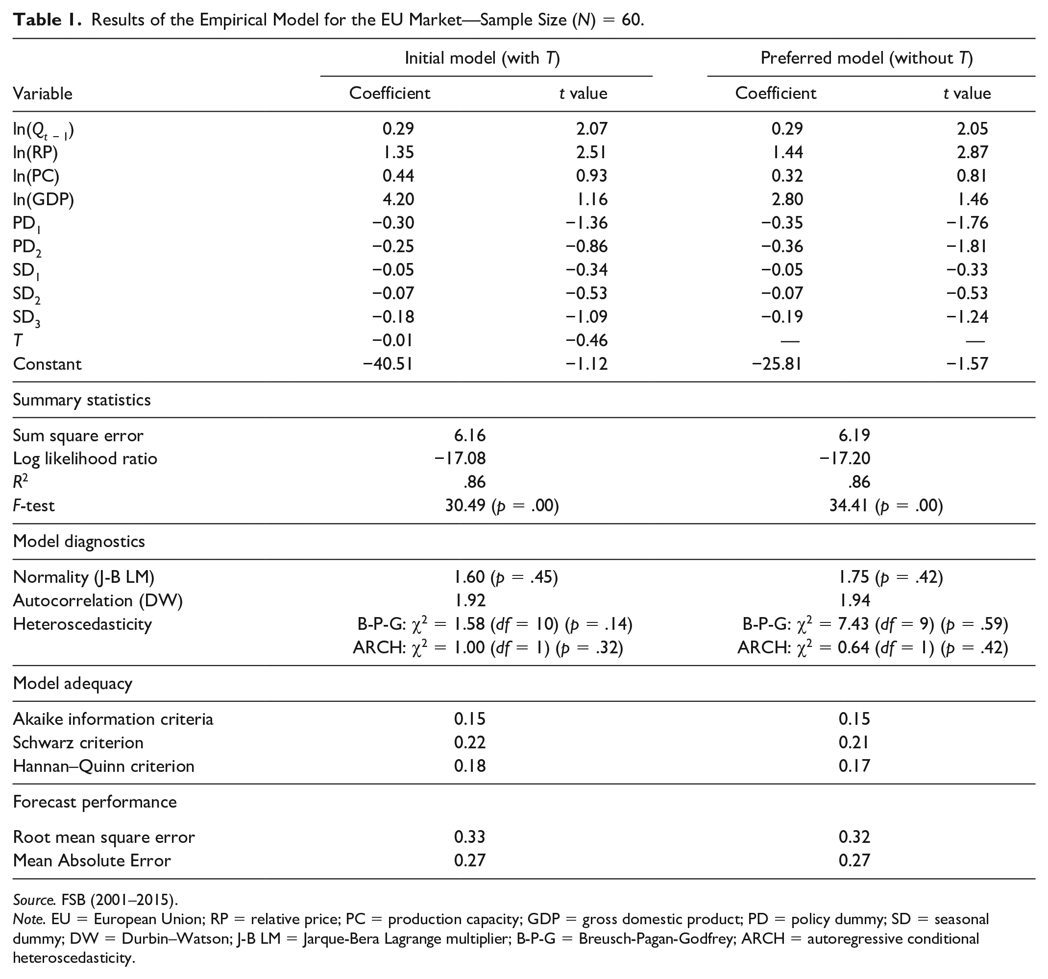
The estimated results from the PAM models (both initial and preferred) along with the corresponding summary statistics, model diagnostics and adequacy, and forecast performance are presented in Tables 1 to 3 for the EU, SEA, and GCC markets, respectively. A number of regression models with various combination of covariates were estimated prior to determining the preferred model based on model diagnostics, and selection criteria such as R² value, sum square error (SSE), likelihood ratio (LR) statistic, Akaike information criteria (AIC), root mean square error (RMSE), and expected sign of the estimates, and so on. It should be noted that the preferred models have satisfied the basic assumptions of the classical regression model as reflected in the results of model diagnostics (Gujarati, 2003). As the results from most of the model selection criteria were in favor of the preferred model, it was decided that the interpretation and discussion of results will be based on the preferred model. It is well-known in time-series literature that the Durbin-Watson (DW) test may not be valid when a time-series model includes lagged dependent variables as one of the explanatory variables. This issue is addressed by computing the Durbin’s h statistics as a test for autocorrelation where appropriate. In case of the SEA market (Table 2), it is found that both test statistics support the hypothesis of “no autocorrelation.” In case of the EU market, the Durbin’s h statistics could not be computed as the square root of a negative number was required. However, given the consistency of the test results for the SEA model, perhaps, it is reasonable to conclude that the model is not suffering from autocorrelation.

Table 1.

Results of the Empirical Model for the EU Market—Sample Size (N) = 60.

Variable	Initial model (with T)		Preferred model (without T)
Variable	Coefficient	t value	Coefficient	t value
ln(Q_t _{− 1})	0.29	2.07	0.29	2.05
ln(RP)	1.35	2.51	1.44	2.87
ln(PC)	0.44	0.93	0.32	0.81
ln(GDP)	4.20	1.16	2.80	1.46
PD₁	−0.30	−1.36	−0.35	−1.76
PD₂	−0.25	−0.86	−0.36	−1.81
SD₁	−0.05	−0.34	−0.05	−0.33
SD₂	−0.07	−0.53	−0.07	−0.53
SD₃	−0.18	−1.09	−0.19	−1.24
T	−0.01	−0.46	—	—
Constant	−40.51	−1.12	−25.81	−1.57
Summary statistics
Sum square error	6.16		6.19
Log likelihood ratio	−17.08		−17.20
R ²	.86		.86
F-test	30.49 (p = .00)		34.41 (p = .00)
Model diagnostics
Normality (J-B LM)	1.60 (p = .45)		1.75 (p = .42)
Autocorrelation (DW)	1.92		1.94
Heteroscedasticity	B-P-G: χ² = 1.58 (df = 10) (p = .14)		B-P-G: χ² = 7.43 (df = 9) (p = .59)
	ARCH: χ² = 1.00 (df = 1) (p = .32)		ARCH: χ² = 0.64 (df = 1) (p = .42)
Model adequacy
Akaike information criteria	0.15		0.15
Schwarz criterion	0.22		0.21
Hannan–Quinn criterion	0.18		0.17
Forecast performance
Root mean square error	0.33		0.32
Mean Absolute Error	0.27		0.27

Source. FSB (2001–2015).

Note. EU = European Union; RP = relative price; PC = production capacity; GDP = gross domestic product; PD = policy dummy; SD = seasonal dummy; DW = Durbin–Watson; J-B LM = Jarque-Bera Lagrange multiplier; B-P-G = Breusch-Pagan-Godfrey; ARCH = autoregressive conditional heteroscedasticity.

Table 2.

Results of the Empirical Model for the SEA Market—Sample Size (N) = 60.

Variable	Initial model		Preferred model
Variable	Coefficient	t value	Coefficient	t value
ln(Q_{t −} ₁)	0.45	4.32	0.47	4.92
ln(RP)	−0.03	−0.05	0.36	0.52
ln(PC)	2.45	4.29	2.39	4.43
ln(GDP)	−2.06	−1.19	−1.75	−3.23
PD₁	0.28	1.12	0.27	1.16
PD₂	0.25	1.01	0.16	0.65
SD₁	−0.59	−2.58	−0.54	−2.92
SD₂	−0.35	−1.80	−0.36	−2.11
SD₃	−0.27	−1.19	−0.28	−1.41
T	0.02	0.41	—	—
DT	—	—	0.01	1.31
Constant	2.86	0.13	−0.20	−0.03
Summary statistics
Sum square error	9.52		9.23
Log likelihood ratio	−29.92		−28.98
R ²	.72		.73
F-test	12.64 (p = .00)		13.20 (p = .00)
Model diagnostics
Normality (J-B LM)	7.09 (p = .03)		1.59 (p = .45)
Autocorrelation: Durbin h (& DW)	0.18 (DW 1.95)		0.02 (DW 1.98)
Heteroscedasticity	B-P-G: χ² = 0.83 (df = 10) (p = .59)		B-P-G: χ² = 18.08 (df = 10) (p = .054)
	ARCH: χ² = 0.25 (df = 1) (p = .62)		ARCH: χ² = 0.05 (df = 1) (p = .83)
Model adequacy
Akaike information criteria	0.23		0.23
Schwarz criterion	0.35		0.33
Hannan–Quinn criterion	0.27		0.26
Forecast performance
Root mean square error	0.43		0.40
Mean absolute error	0.34		0.30

Source. FSB (2001–2015).

Note. SEA = Southeast-, East- and South Asia; RP = relative price; PC = production capacity; GDP = gross domestic product; PD = policy dummy; SD = seasonal dummy; DT = dummy variable; DW = Durbin–Watson; J-B LM = Jarque-Bera Lagrange multiplier; B-P-G = Breusch-Pagan-Godfrey; ARCH = autoregressive conditional heteroscedasticity.

Table 3.

Results of the Empirical Model for the GCC Market—Sample Size (N) = 60.

Variable	Initial model (with SD and T)		Preferred model (without SD and T)
Variable	Coefficient	t value	Coefficient	t value
ln(Q_{t −} ₁)	0.001	0.007
ln(RP)	0.43	2.18	0.22	1.19
ln(PC)	0.07	0.43	0.45	3.79
ln(GDP)	0.35	2.51	0.43	6.06
PD₁	0.07	0.99	0.01	0.16
PD₂	0.16	1.98	0.18	2.60
SD₁	0.02	0.35	—	—
SD₂	−0.07	−1.27	—	—
SD₃	−0.18	−2.80	—	—
T	0.01	1.06	—	—
Constant	6.58	3.00	2.32	1.98
Summary statistics
Sum square error	0.83		1.05
Log likelihood ratio	41.93		34.95
R ²	.89		.86
F-test	40.00 (p = .00)		67.49 (p = .00)
Model diagnostics
Normality (J-B LM)	20.05 (p = .00)		0.89 (p = .64)
Autocorrelation: Durbin h (& DW)	NA (DW 2.08)		NA (DW 2.02)
Heteroscedasticity	B-P-G: χ² = 0.93 (df = 10) (p = .52)		B-P-G: χ² = 0.95 (df = 6) (p = .47)
	ARCH: χ² = 0.18 (df = 1) (p = .68)		ARCH: χ² = 0.14 (df = 1) (p = .71)
Model adequacy
Akaike information criteria	0.02		0.02
Schwarz criterion	0.03		0.03
Hannan–Quinn criterion	0.02		0.02
Forecast performance
Root mean square error	0.12		0.13
Mean absolute error	0.09		0.11

Source. FSB (2001–2015).

Note. GCC = Gulf Cooperation Council; RP = relative prices; PC = production capacity; GDP = gross domestic product; PD = policy dummy; SD = seasonal dummy; DW = Durbin–Watson; J-B LM = Jarque-Bera Lagrange multiplier; B-P-G = Breusch-Pagan-Godfrey; ARCH = autoregressive conditional heteroscedasticity; NA = not applicable.

A legitimate question can be raised regarding the bias in coefficient estimates due to the small sample size and data aggregation. In examining the small sample bias due to misspecification of the PAM and adaptive expectations models, Waud (1966) observed that departures from normality in the distribution of the coefficient of adjustment parameter are considerably less noticeable and significant for samples of size 60 as opposed to sizes of 20 and 30. With regard to data aggregation bias, in the presence of heterogeneity among countries within a region, aggregation of time-series data to a regional level might mitigate the biases in estimates by reducing parameter heterogeneity (Hendricks et al., 2014). Furthermore, no attempt is being made to generalize the results from the regional-level investigation to the country level to avoid erroneous inferences associated with the aggregation problem (Clark & Avery, 1976). More importantly, the grouping of countries in this study was not random but rather systematic in which the main criterion for grouping is spatial proximity which is most likely to be of particular interest to policy makers and seafood businesses.

Table 1 presents the preferred model for the EU market. It is noted that the lagged dependent variable “ $\ln (Q_{t - 1})$ ” and the relative price variable “ln(RP)” were significant at the 1% and 5% level, respectively. Furthermore, both policy variables “PD₁” and “PD₂” were significant at 5% level.

Table 2 presents the results for the SEA market. It is important to note that the initial model (with time trend) violates the assumption of residuals normality. To rectify this problem, an interactive dummy variable (DT) with “T” (where D = 1 from 2007 onward and “0” otherwise) was introduced based on the observation of export behavior that reveals that the export trend stopped declining and became stable since 2007 and started to increase in 2011 (Figure 2). The introduction of the DT variable in the preferred model corrects the residuals normality problem. It should be noted that in the preferred model, four explanatory variables, namely, the lagged dependent variable “ $l n (Q_{t - 1})$ ,” production capacity “ln(PC),” gross domestic product “ln(GDP),” and seasonal dummies “SD₁” and “SD₂” were significant at the 5% level.

The results for the GCC market are presented in Table 3. It is worth mentioning that the initial model failed to produce white noise errors. After experimentation with various combinations of variables it was revealed that the seasonal dummies and time trend variables were interfering with the normality of residuals. Therefore, those variables were excluded from the preferred model. It is noted that the lag dependent variable was insignificant in the preferred model. Therefore, the model was also experimented without the lag dependent variable but there was no improvement in the results. Hence, it was decided to exclude the lag dependent variable from the model to increase the degrees of freedom. In the preferred model, the production capacity “ln(PC),” gross domestic product “ln(GDP),” and the policy variable “PD₂” were significant at the 5% level.

Table 4 summarizes the empirical findings. The results indicate a lack of homogeneity across markets as the export-supply is influenced by factors that are uncommon across markets.

Table 4.

Summary Results of Significant Variables in the Models.

Variable	EU market	GCC market	SEA market
ln(Q_{t −} ₁)	Yes	No	Yes
ln(RP)	Yes	No	No
ln(PC)	No	Yes	Yes
ln(GDP)	No	Yes	Yes
PD₁	Yes	No	No
PD₂	Yes	Yes	No
SD₁	No	—	Yes
SD₂	No	—	Yes
SD₃	No	—	No

Source. Compiled from empirical models.

Note. EU = European Union; GCC = Gulf Cooperation Council; SEA = Southeast-, East- and South Asia; RP = relative price; PC = production capacity; GDP = gross domestic product; PD = policy dummy; SD = seasonal dummy.

Discussion

The following section will discuss the results generated through descriptive and empirical analysis along with the conformity (or otherwise) to the key hypotheses. The lack of homogeneity across markets, perhaps, signals important differences in consumer preferences which may be influenced by socioeconomic, demographic, cultural, psychological, and market-related factors (Yousuf et al., 2019). Culture and geographical location of consumers can also exert influence on preferences for seafood (Cardoso et al., 2013) and such cross-cultural differences may act as a barrier to global market homogeneity (Shaw & Clarke, 1998).

The empirical results with regard to the lag dependent variable showed that the variable conveys an expected sign in all cases but is statistically significant in the EU and SEA models. The speed of the adjustment which is completed in one period is about 71.2% (with the average lag being about 0.41 quarter) and 52.5% (with the average lag being about 0.01 quarter) for the EU and SEA markets, respectively. This result suggests that the supply response to the SEA market requires less adjustment time than the EU market. This result is not unusual as the speed of adjustment is influenced by the extent of adjustment costs which in turn is influenced by factors such as distance, transportation costs, availability fish products, government export policies, and so on. In the case of New Zealand lobster export to Japan, Bose and Galvan (2005) noted that 39% of the gap between the actual and desired level was covered in each period. For the EU market case using yearly data, Bose et al. (2019) found that the average lag is about 1.4 years. The insignificance of adjustment lag suggests that exporters’ expectations become irrelevant and exporters have no interest in predicting future conditions of the GCC market.

It should be noted that the relative price variable “ln(RP)” measures the responsiveness of the export-supply with respect to the export price relative to domestic price in the short-run (for the model with lag dependent variable), ceteris paribus. Although the positive sign of the estimated coefficient for all cases is consistent with the economic theory of supply, the coefficient is significant for the EU market only. It indicates that a 1% increase in the relative price, other things being equal, will stimulate a 1.44% increase in the export-supply to the EU market. It also reflects the fact that the price of seafood products in the EU market was attractive to encourage producers to supply their products relative to domestic price and is consistent with the notion of high-value market as labeled by others (Qatan et al., 2015). In addition, the result in relation to positive growth rate of price compared with quantity in the EU market factor signals the importance of the price factor in this market.

The coefficient of production capacity measures the short-run elasticity of export-supply with respect to production capacity (for the model with lag dependent variable). Although the estimated coefficient for all markets carries the expected positive sign, the coefficient is significant for the SEA and GCC markets only. In addition, the responsiveness was about 5 times higher in the SEA market than that of the GCC market. The implication of this finding is that any decrease in the total landings, other things being equal, could have a negative impact on both markets with varying extent. The inelastic result for the GCC market is not uncommon. Bose and Galvan (2005) found that the coefficient of productive capacity was inelastic (0.17) in the export-supply model of live rock lobster.

The estimated coefficient of the seafood export-supply with respect to market size carries a positive sign for the EU and GCC markets but the opposite holds true for the SEA market. Furthermore, it is statistically significant for the SEA and GCC markets only. The negative sign of the estimated coefficient for the SEA market perhaps reflects the change in consumer preference structure due to GDP growth as predicated by Delgado et al. (2003). It is projected that there will be a higher growth in consumption of high-value fish species compared with low-value species (1.7% vs. 1.4% per annum) in the SEA market (Delgado et al., 2003). This finding should not be surprising as increases in standard of living tend to generate a desire for high-value fish products. The finding is consistent with descriptive statistical results (Figure 5) which show that the export of small pelagic species was dominant over the study period. However, further analysis revealed an upward trend in case of large pelagics and demersal species in the SEA market during the last part (2011–2015) of the study period.

The inelastic export-supply with regard to market size in the GCC model indicates that the increase in the market size by 1% will increase the export-supply by 0.43%, other things being equal. With regard to the policy variable “PD₁” that represents the domestic export ban, the estimated coefficient for the EU market is found to be negative as expected and statistically significant at the 5% level (one-tailed). However, the estimated coefficient for the SEA and GCC models was found to be insignificant with a positive sign. Therefore, the results provide support to Research Hypothesis 1 only for the EU market. This is consistent with the findings by Bose et al. (2019) who noted the domestic export ban rather than the border rejections by the EU countries has acted as a significant barrier to fish exports to the EU. A recent study conducted by Al-Busaidi et al. (2017) stated that the share of Oman’s end products going to lucrative markets such as the EU, the United States, and Japan declined due to the exports ban on specific species. The present finding signals competition between the EU and the domestic market as strong consumer preferences exist in the domestic market for those demersal and large pelagic species that are being exported to the EU market (Bose et al., 2010; Yousuf et al., 2019). In addition, the ban on fish exports hinders regularity of exports to the EU market, which may not be favored by the EU traders. Bose et al. (2019) pointed out that the higher the extent of demand for those species in the local market is, the greater will be the competition and that will lead to more irregularity of supply to the EU as more of the same product will be diverted toward the domestic market.

With regard to the demesral trawl fishing ban represented by the second policy variable “PD₂,” the coefficient carries a negative sign for the EU market and is statistically significant at the 5% level. However, with regard to the sign of the estimated coefficient, the opposite holds true for the GCC and SEA cases and it is significant only for the GCC market. Nevertheless, with regard to the EU and GCC markets, the results lend support to Research Hypothesis 2. For the GCC market, the result is not unexpected. As noted earlier, the GCC market was dominated by small pelagics, followed by demersal species, while the trawl fishery landings were particularly demersal species and primarily supplied to the EU market. Therefore, the ban was expected to have a negative impact on the export of demersal species, which is highly demanded by the EU market as mentioned previously (Figure 4). In addition, the demersal trawl fishery was very effective in maintaining the freshness of the fish, as vessels had high capacity of storing and preserving fish in a proper manner using ice compared with traditional fishery which is mainly dominated by small-scale fishers who use small boats incapable of the proper handling of fish. Besides that, in Western countries such as Australia and New Zealand, consumers are very concerned about the quality of the seafood products, which is perceived as “freshness” (Bose & Brown, 2000; Spinks & Bose, 2002). Moreover, it was found that the EU market demands very high-quality and safe seafood products (Qatan et al., 2015). Hence, the decline in export to the EU countries was apparent due to the trawl ban, which led to the lack of freshness of demersal species landed by the artisanal sector as mentioned earlier.

Although, there was a continuous supply of the demersal species in terms of quantity from the artisanal fishery, the freshness of the demersal species supplied to the EU market has been affected since the ban was imposed. Furthermore, since the trawl ban, the introduction of coastal fishery has been gradually contributing to the demersal fish catch (Al-Masroori & Bose, 2016). However, the contribution of the coastal fishery is still very small, and it reached only 0.8% of the total fish landings in 2016 (FSB, 2000–2016).

Conversely, for the GCC market, the positive sign of the coefficient indicates that the imposition of trawl ban policy since 2009 enhanced the total quantity of seafood products supplied to this market. The increase of the export-supply to the GCC market confirms what has been explained above in relation to the continuity of export-supply of the demersal species from other fisheries subsectors, in particular the artisanal sector, as this market is less stringent about the freshness of fish products.

In view of that, it can be said that the effect of a specific demersal species ban is relatively powerful for the EU market compared with the GCC as the ban is compounded with the other factor (i.e., freshness). With particular reference to the EU market, the results support Research Hypothesis 2.

The seasonal dummy variables were used to capture the effect of the seasonal variation in the export-supply of seafood products to each market. It was found that there is a significant seasonal variation of the seafood export-supply to the SEA market only. It is noted that the export-supply is relatively low during the first and second quarters compared with the last quarter.

There is a significant seasonal variation of the seafood export-supply to the SEA market which is relatively low during the first and second quarters compared with the last quarter. This could be due to the fact that the highest proportions of exported species to this market are small pelagics (dominated by sardine, Indian mackerel, and small jacks), followed by crustaceans and molluscs (dominated by cuttlefish; Figure 5). The landings of dominant small pelagic species are usually during the third and fourth quarters of the year and sometimes extended to the first quarter, and the highest landings of cuttlefish are during the last quarter of each year (FSB, 2000–2016). Therefore, this seasonality is driven by supply-side issue such as landings of some particular species. This result is consistent with the findings of the work conducted by Bose and Galvan (2005) to investigate export-supply of rock lobster from New Zealand to Japan, and Bose and Redkar (2004) to estimate the Japanese import demand for Indian seafood products.

Policy Issues

This section discusses some key policy issues based on the key findings of this study. A lack of market homogeneity as noted may not be due solely to differences in safety and quality standards, and it is also plausible that other socioeconomic conditions and market preferences can disturb market homogeneity. For instance, the descriptive analysis of the export of each fish category revealed that market preference for species in the EU which was dominated by the demersal species was different from the SEA and GCC markets that were dominated by small pelagic species. The policy implication of such heterogeneity across markets is that one-size-fits-all approach would not be effective. Instead, it requires market-specific strategy.

It was also found that two policy measures, namely, the export ban and trawl fishing ban have been instrumental in bringing change in the EU market—once Oman’s preferred fish export destination. The significant influence of the export restraints and trawl fishing ban on the export-supply to the EU market suggests that such regulatory measures are a source of tension between the domestic and the EU markets. It should be mentioned that the supply of protection in the form of export restraints has its own costs and benefits. There is a trade-off between the protection of domestic consumers and the revenue forgone. The apparent trade-off, as the result showed, is in the form of reduced market share and low foreign exchange earnings. Therefore, it is important to determine the costs of introducing an export ban and such costs should be balanced by the benefits it generates through serving domestic consumers and/or self-sufficiency in food (SCP, 2018). For instance, in 2016, the self-sufficiency of seafood products in Oman was estimated to be about 176% and per capita consumption was 35.7 kg/year (FSB, 2000–2016) which are of national interests under the present food security campaign (Bose et al., 2010).

Although such measures could achieve the objective of protecting domestic consumers’ interests and food and nutritional security which is an important strategic objective of the fisheries sector (Bose et al., 2010; SCP, 2018), these policy measures produce market failure and, therefore, fail to provide an effective mechanism to assure the balancing of costs and benefits (Friedman & Friedman, 1980). Such interventions may also produce economic efficiency loss by affecting efficient allocation of fish products. In addition, the distributional effects of protection remain unknown. If the expectation of local seafood businesses regarding such intervention is not temporary, then they will have to make necessary adjustments to export-supply and such decisions involve adjustment costs. Furthermore, it also involves considerable transaction costs (i.e., enforcement and monitoring costs) in the form of designing, implementing, and monitoring the effectiveness of such measures. Therefore, a cost-effective policy must be designed not only to minimize any adverse economic effects on the earnings of the domestic seafood businesses but also minimize the transaction costs. However, if the costs associated with such measures outweigh the benefits, the government intervention can only be justified based on a social welfare perspective.

From the perspective of the EU market, if the EU importers’ expectation of the market intervention is not temporary, the EU seafood business may react by switching to the other supply sources if the interventions adversely affect the welfare of the EU consumers and create supply uncertainty. Therefore, if it is desirable to preserve the EU market, the authority must find ways that are mutually beneficial.

There are certain actions that could be followed in the process of reducing market tension. For instance, effective promotional campaigns by local seafood businesses in the EU could be assisted through an appropriate government assistance scheme to persuade change in the preference structure of the EU consumers for various nontraditional new species. This approach can also be applied to domestic market through an awareness program. Based on a local case study, Yousuf et al. (2019) found that unfamiliarity with species, cooking experience, and strong preferences for selected fish species have limited consumers’ preference set and, thus, suggested marketing strategies like distributing seafood recipe cards, establishing seafood testing counters at supermarkets and encouraging trials, setting up cooking displays and so on. as educative measures. Although an attempt to introduce species not traditionally exported to foreign markets involves uncertainties (i.e., taste and preferences, appropriate nomenclature) and is a time-consuming task as the change may not be immediate, the approach is not unusual as it was experienced by the Gulf and South Atlantic Fisheries Development Foundation during 1979 and 1980, and many of these uncertainties were overcome with time (Prochaska, 1984).

A policy issue with regard to the production capacity (proxied by total fish landings) variable is that the enhancement strategy of export-supply needs to be in line with fish stocks conditions and the long-term sustainability of fish resources. The result in relation to the dominance of the growth rate in quantity rather than that of price in the two markets (SEA and GCC) suggests that the government should consider the price improvement strategy through value-added products to increase export revenue without undermining the long-term sustainability of fisheries resources.

Shift in consumer preferences can also be brought about by various factors, including product image through certification, product promotion involving product safety and high quality, and the like. It should be noted that the expected growth in GDP and demand for high-quality and high-value fish in case of the SEA market by Delgado et al. (2003) attracts competitors. In this context, export of high-quality and high-value fish by Omani seafood companies with the HACCP system may set new standards and could create a competitive edge in the market that has the potential to payoff nicely for the seafood companies in Oman. Furthermore, similarity in market preferences of un-banned species, particularly in the SEA and the GCC market, should also offer a competitive advantage to Omani seafood exporters.

Concluding Remarks

With the growing consumer interest in fish and seafood products as a source of nutrition, it is imperative for both the authority and seafood businesses to have a clear conception of export market behavior. This article has empirically examined the significant influence of domestic regulatory measures, relative prices, market size, seasonality, and time trends on the export-supply of Omani seafood products to three selected markets, namely, the EU, SEA, and the GCC covering the period 2001–2015. Following the nested hypothesis test result, the Cobb–Douglas-type functional specification was used under a PAM approach. The model was estimated using ordinary least square (OLS).

The descriptive statistical results indicate market heterogeneity in species preferences. The empirical results suggest some degree of inertia in adjustment in the EU and SEA markets. It is also found that domestic bans on fish export exert a negative impact on the EU market only, and hence this finding lends partial support to the first research hypothesis. The “trawl fishing ban” is found to negatively (positively) impact the seafood export to the EU (the GCC) market, which provides support to the second research hypothesis. The significance of “production capacity” for the GCC and SEA markets deserves careful attention as any future enhancement strategies in relation to fish exports need to be in line with the long-term sustainability of fish resources.

However, two limitations of this study that relate to the data are as follows. First, the present study covers only three broadly classified regional markets based on the grouping of countries with geographical proximity. Second, the empirical analysis is based on aggregated data generated from the grouping of countries. The lack of uninterrupted country-specific export data prohibits the county-specific supply analysis. An implication of such limitations is that it prohibits the formulation of any country-specific policy strategies to improve the export potential for fish products in the concerned country. However, if suitable data were available, country-specific estimates could be obtained by simply replicating the modeling procedure. Despite these limitations, concerned authorities and seafood companies should find the findings of this study useful for developing effective policies to address market heterogeneity and maximize export revenue on, at least, a regional basis. For instance, knowledge about speeds of adjustment, heterogeneity in species preferences, and extent of supply responsiveness to the relative prices, market size, and production capacity help policy makers in the design of appropriate stabilization policies for regional export markets.

The present findings can be further enriched by checking the robustness of the present findings by employing the ECM of Engle and Granger (1987) as its error-correction term represents the adjustment costs and provides the link between short- and long-run analysis. In the context of agricultural supply response analysis, the application of such an approach can be found in Hallam and Zanoli (1993), Gunawardana, et al. (1995), and Olubode-Awosola, et al. (2006), just to name a few. In addition, as the fishing industry has been exposed to various types of risks (Prochaska, 1984), an examination of the sensitivity of export-supply to potential risks along the lines of Ryan (1977) and Antonovitz and Green (1990) should also be a useful addition to the present research.

Footnotes

Authors’ Note

S. B. was working at the Sultan Qaboos University while the initial submission and the first revision made to the submitted manuscript.

Declaration of Conflicting Interests

The author(s) declared no potential conflicts of interest with respect to the research, authorship, and/or publication of this article.

Funding

The author(s) received no financial support for the research, authorship, and/or publication of this article.

ORCID iD

Shekar Bose

References

Abeysinghe

Rajaguru

(2004). Quarterly real GDP estimates for China and ASEAN4 with a forecast evaluation. Journal of Forecasting, 23(6), 431–447.

Al-Busaidi

M. A.

Jukes

D. J.

Bose

(2016). Seafood safety and quality: An analysis of the supply chain in the Sultanate of Oman. Food Control, 59, 651–662.

Al-Busaidi

M. A.

Jukes

D. J.

Bose

(2017). Hazard analysis and critical control point (HACCP) in seafood processing: An analysis of its application and use in regulation in the Sultanate of Oman. Food Control, 73, 900–915.

Al-Masroori

H. S.

Bose

(2016). Anchoring to determine negotiated catch limits: A case study of an industrial fishery in Oman. African Journal of Marine Science, 38(1), 101–109.

Alogoskoufis

Smith

(1991). On error correction models: Specification, interpretation, estimation. Journal of Economic Surveys, 5(1), 97–128.

Al-Subhi

K. K. N.

Bose

Al-Masroori

H. S.

(2013). Fishers’ compliance motivations: A case study of the Sultanate of Oman. Marine Policy, 37, 141–148.

Antonovitz

Green

(1990). Alternative estimates of fed beef supply response to risk. American Journal of Agricultural Economics, 72(2), 475–487.

Askari

Cummings

J. T.

(1977). Estimating agricultural supply response with the Nerlove model: A survey. International Economic Review, 18:, 257–292.

Bond

M. E.

(1987). An econometric study of primary commodity exports from developing country regions to the world. IMF Staff Papers, 34(2), 191–227.

10.

Bose

Al-Mazrouai

Al-Habsi

Al-Busaidi

Al-Nahdi

(2010, March). Fisheries and food security: The case of the Sultanate of Oman [Conference session]. International Conference on Food Security in the Arab Countries: New Challenges and Opportunities in the Context of Global Price Volatility, Muscat, Sultanate of Oman.

11.

Bose

Al Naabi

A. M. R.

Boughanmi

Yousuf

J. B.

(2019). Domestic ban versus border rejections: A case of Oman’s fish exports to the EU. SAGE Open, 9(1), 1–12.

12.

Bose

Brown

(2000). A preliminary investigation of factors affecting seafood consumption behaviour in the inland and coastal regions of Victoria, Australia. International Journal of Consumer Studies, 24(4), 257–262.

13.

Bose

Galvan

(2005). Export supply of New Zealand’s live rock lobster to Japan: An empirical analysis. Japan and the World Economy, 17(1), 111–123.

14.

Bose

Redkar

(2004, July 20–30). Modelling Japanese import demand function for Indian seafood products [Conference session]. IIFET 2004 Japan Conference, Tokyo, Japan.

15.

Cardoso

Lourenço

Costa

Gonçalves

Nunes

M. L.

(2013). Survey into the seafood consumption preferences and patterns in the Portuguese population: Gender and regional variability. Appetite, 64, 20–31.

16.

Carone

(1996). Modeling the US demand for imports through cointegration and error correction. Journal of Policy Modeling, 18(1), 1–48.

17.

Chambers

R. G.

Lopez

R. E.

(1984). A general, dynamic, supply-response model. Northeastern Journal of Agricultural and Resource Economics, 13, 142–154.

18.

Clark

W. A.

Avery

K. L.

(1976). The effects of data aggregation in statistical analysis. Geographical Analysis, 8(4), 428–438.

19.

Colman

(1983). A review of the arts of supply response analysis. Review of Marketing and Agricultural Economics, 51(3), 201–230.

20.

De Menezes

T. A.

Piketty

M. G.

(2012). Towards a better estimation of agricultural supply elasticity: The case of soya beans in Brazil. Applied Economics, 44(31), 4005–4018.

21.

Delgado

C. L.

Wada

Rosegrant

M. W.

Meijer

Ahmed

(2003). Fish to 2020. World Fish Centre; International Food Policy Research Institute.

22.

Diebold

F. X.

Lamb

R. L.

(1997). Why are estimates of agricultural supply response so variable? Journal of Econometrics, 76(1–2), 357–373.

23.

Doran

H. E.

(1988). Specification tests for the partial adjustment and adaptive expectations models. American Journal of Agricultural Economics, 70(3), 713–723.

24.

Eckstein

(1985). The dynamics of agriculture supply: A reconsideration. American Journal of Agricultural Economics, 67(2), 204–214.

25.

Engle

R. F.

Granger

C. W. J.

(1987). Co-integration and error correction: Representation, estimation, and testing. Econo-metrica, 55(2), 251–276.

26.

Estrella

Fuhrer

J. C.

(2002). Dynamic inconsistencies: Counterfactual implications of a class of rational-expectations models. American Economic Review, 92(4), 1013–1028.

27.

Friedman

(1980). Free to choose: A personal statement. Harcourt Brace Jovanovich.

28.

Fisheries Statistics Yearbook (FSB). (2000–2016). Fishery statistics books—Several years. Fisheries Statistics and Information Department, Ministry of Agriculture and Fisheries.

29.

Gilbert

C. L.

(1986). Practitioners’ corner: Professor Hendry’s econometric methodology. Oxford Bulletin of Economics and Statistics, 48(3), 283–307.

30.

Gosalamang

D. S.

Belete

Hlongwane

J. J.

Masuku

(2012). Supply response of beef farmers in Botswana: A Nerlovian partial adjustment model approach. African Journal of Agricultural Research, 7(31), 4383–4389.

31.

Griffiths

W. E.

Anderson

J. R.

(1978). Specification of agricultural supply functions-empirical evidence on wheat in Southern NSW. Australian Journal of Agricultural Economics, 22(2–3), 115–128.

32.

Gujarati

D. N.

(2003). Basic econometrics (4th ed.). McGraw-Hill.

33.

Gunawardana

P. J.

Kidane

Kulendran

(1995). Export supply response of the Australian citrus industry. Australian Journal of Agricultural Economics, 39(3), 247–261.

34.

Hallam

Zanoli

(1993). Error correction models and agricultural supply response. European Review of Agricultural Economics, 20(2), 151–166.

35.

Hendricks

N. P.

Smith

Sumner

D. A.

(2014). Crop supply dynamics and the illusion of partial adjustment. American Journal of Agricultural Economics, 96(5), 1469–1491.

36.

Hendry

D. F.

von Ungern-Sternberg

(1981). Liquidity and inflation effects on consumer’s expenditure. In Deaton

A. S.

(Ed.), Essays in the theory and measurement of consumer’s behaviour (pp. 237–260). Cambridge University Press.

37.

Just

R. E.

(1977). Estimation of an adaptive expectations model. International Economic Review, 18(3), 629–644.

38.

Kennan

(1979). The estimation of partial adjustment models with rational expectations. Econometrica, 47(6), 1441–1455.

39.

Kennedy

P. E.

(2002). Sinning in the basement: What are the rules? The ten commandments of applied econometrics. Journal of Economic Surveys, 16(4), 569–589.

40.

King

R. G.

Thomas

J. K.

(2006). Partial adjustment without apology. International Economic Review, 47(3), 779–809.

41.

Kmenta

(1967). On estimation of the CES production function. International Economic Review, 8(2), 180–189.

42.

La France

J. T.

Burt

O. R.

(1983). A modified partial adjustment model of aggregate US agricultural supply. Western Journal of Agricultural Economics, 8(1), 1–12.

43.

Lahari

Haug

A. A.

Garces-Ozanne

(2011). Estimating quarterly GDP Data for the South Pacific Island Nations. The Singapore Economic Review, 56(01), 97–112.

44.

Lawrence

(1990). An adjustment-costs model of export supply and import demand. Journal of Econometrics, 46(3), 381–398.

45.

Mbaga

Coyle

B. T.

(2003). Beef supply response under uncertainty: An autoregressive distributed lag model. Journal of Agricultural and Resource Economics, 28(3), 519–539.

46.

Ministry of Agriculture and Fisheries. (2015). Ninth five-year plan (2016-2020).

47.

Ministry of Agriculture and Fisheries. (2018). Directorate general of fisheries marketing and investment.

48.

Muth

J. F.

(1961). Rational expectations and the theory of price movements. Econometrica, 29(3), 315–335.

49.

Nerlove

(1956). Estimates of the elasticities of supply of selected agricultural commodities. Journal of Farm Economics, 38(2), 496–509.

50.

Nerlove

(1979). The dynamics of supply: Retrospect and prospect. American Journal of Agricultural Economics, 61(5), 874–888.

51.

Nichell

(1985). Error correction, partial adjustment and all that: An expository note. Oxford Bulletin of Economics and Statistics, 47(2), 119–129.

52.

Olubode-Awosola

O. O.

Oyewumi

O. A.

Jooste

(2006). Vector error correction modelling of Nigerian agricultural supply response. Agrekon, 45(4), 421–436.

53.

Phlips

(1974). Applied consumption analysis. North Holland Publishing.

54.

Prochaska

F. J.

(1984). Principal types of uncertainty in seafood processing and marketing. Marine Resource Economics, 1(1), 51–66.

55.

Qatan

Bose

Mothershaw

(2015). Stakeholders’ views on the status of the fish quality and safety regulatory schemes: The case of the sultanate of Oman. British Food Journal, 117(4), 1303–1314.

56.

Ryan

T. J.

(1977). Supply response to risk: The case of US pinto beans. Western Journal of Agricultural Economics, 2, 35–43.

57.

SCP. (2018). https://www.scp.gov.om/PDF/Economic%20Diversification%20Sector%20Book-EN.pdf

58.

Shaw

D. S.

Clarke

(1998). Culture, consumption and choice: Towards a conceptual relationship. International Journal of Consumer Studies, 22(3), 163–168.

59.

Shideed

K. H.

White

F. C.

(1989). Alternative forms of price expectations in supply analysis for US corn and soybean acreages. Western Journal of Agricultural Economics, 14(2), 281–292.

60.

Shoko

R. R.

Chaminuka

Belete

(2016). Estimating the supply response of maize in South Africa: A Nerlovian partial adjustment model approach. Agrekon, 55(3), 237–253.

61.

Shonkwiler

J. S.

(1982). An empirical comparison of agricultural supply response mechanisms. Applied Economics, 14(2), 183–194.

62.

Shumway

C. R.

Chang

A. A.

(1977). Linear programming versus positively estimated supply functions: An empirical and methodological critique. American Journal of Agricultural Economics, 59(2), 344–357.

63.

Spinks

Bose

(2002). Factors affecting households’ seafood purchasing decisions in Auckland, New Zealand: An empirical analysis. International Journal of Consumer Studies, 26(1), 62–70.

64.

Thiele

(2000, December). Estimating the aggregate agricultural supply response: A survey of techniques and results for developing countries (No. 1016, Kiel Working Paper). https://www.econstor.eu/bitstream/10419/2516/1/kap1016.pdf

65.

Thursby

(1984). How reliable are simple, single equation specifications of import demand? The Review of Economics and Statistics, 66(1), 120–128.

66.

Waud

R. N.

(1966). Small sample bias due to misspecification in the “partial adjustment” and “adaptive expectations” models. Journal of the American Statistical Association, 61(316), 1130–1152.

67.

Wickens

M. R.

Greenfield

J. N.

(1973). The econometrics of agricultural supply: An application to the world coffee market. The Review of Economics and Statistics, 55(4), 433–440.

68.

Yousuf

J. B.

Bose

Kotagama

Boughanmi

(2019). Preferences and intentions of seafood consumers in Oman: An empirical analysis. Journal of International Food & Agribusiness Marketing, 31(2), 175–203.

Do Regulatory Measures Necessarily Affect Oman’s Seafood Export-Supply?

Abstract

Keywords

Introduction

Brief Review of Relevant Studies

Data Description

Empirical Model

Results

Descriptive

Empirical

Discussion

Policy Issues

Concluding Remarks

Footnotes

Authors’ Note

Declaration of Conflicting Interests

Funding

ORCID iD

References