Liquidity and Firms’ Financial Performance Nexus: Panel Evidence From Non-Financial Firms Listed on the Ghana Stock Exchange

Abstract

The aim of this research was to establish the nexus between liquidity and the viability of quoted non-financial establishments in Ghana. Panel data deduced from the published annual reports of 15 entities for the period 2008 to 2017 was employed for the study. Preliminarily, cross-sectional reliance, unit root, serial correlation, heteroscedasticity, co-integration, and causality tests were respectively performed. Our findings established that there exists no cross-sectional reliance, and input variables are stationary and co-integrated with no presence of heteroscedasticity and serial correlation. Estimates from the random effects generalized least squares (GLS) regression showed that liquidity has significant adverse effect on the firms’ Return on Equity (ROE) but had insignificantly positive effect on ROE when surrogated by the cash flow ratio. Finally, test based on causalities uncovered that, with the exception of Current Ratio and ROE that are flanked by bidirectional liaison, no other causal affiliation was evidenced amid other variables. Policy recommendations are further discussed.

Introduction

The necessity of liquidity and its influence on the financial performance of organizations cannot be underrated (Kimondo et al., 2016). This is because liquidity forms an imperative part in the development and improvement of corporations. As such, the proper administration of firms’ resources is very crucial, because it will ensure that there is adequate liquidity for the firms to fulfill their immediate financial obligations without a default (Apuoyo, 2010; Bhunia et al., 2011; Orshi, 2016). Akenga (2017), Alshatti (2015), and Ehiedu (2014) viewed liquidity as the capability of an establishment to pay its immediate financial commitment when it is matured for settlement by converting short-term assets into cash without incurring any loss. According to the authors, a firm that is able to meet its immediate financial commitments upon maturity is considered liquid, and creates a good image for itself in the face of customers and creditors. As indicated by Bhunia et al. (2011), Orshi (2016), Apuoyo (2010), Akenga (2017), Alshatti (2015), and Ehiedu (2014), assets are considered liquid and of high quality when they can be simply and directly changed into cash at little or no loss of value. In the same vain, markets are considered liquid when individuals operating in those markets can defray their assets at prices that would result in a gain.

The undertakings of firms is embedded with several obligations among some are the meeting of daily operational costs, unforeseen emergencies, contingencies, or accidents. In order for such obligations to be met efficiently and effectively, the firms are required to be liquid enough (Akenga, 2017). Profitability of firms may be improved for holding liquid assets; however, it gets to a point at which the holding of more of such liquid assets adversely affect firms’ profitability. Thus, firms can achieve the “twin conflicting” objective of liquidity and improved financial performance by coming out with a more diversified and a balanced asset–liability mix, where they will be able to meet their financial obligations and still remain liquid and profitable (Akenga, 2017; Alshatti, 2015; Apuoyo, 2010; Ehiedu, 2014; Njoroge, 2015; Omesa, 2015; Orshi, 2016).

Prevailing practical occurrences have of late shown that, some non-financial firms listed on the Ghana Stock Exchange (GSE) are faced with the challenge of effectively managing their liquidity to attain improved financial performance. This scenario is evidenced by the complete delisting of Golden Web Ghana Ltd, Transaction Solutions Ghana Ltd, Pioneer Kitchenware Company Limited, Aluworks Ltd, and Cocoa Processing Company Ltd by the stock regulator, as a result of their failure to rectify some identified anomalies within a given time frame of which poor liquidity positions played a key role. Prior to their delisting, the aforementioned companies alongside Clydestone Ghana Ltd had been technically suspended from the stock market. Cocoa Processing Company Ltd which was suspended from trading in August 2017 had failed to submit its audited financial and operational results for the years 2015 and 2016. As of May 2017, the firm owed a consortium of lending banks some US$20 million. Aluworks also blamed its ongoing financial struggles on unfair trade practices, submitting that Ghana has become a dumping ground for cheaper aluminum products particularly from Nigeria and some other parts of the world.

Apart from the above, companies like Ayrton Drugs Manufacturing Company Ltd and Golden Star Resources have had ceaseless changes in their financial years of operations which have affected their trend records, and have also been reluctant to file their complete financial reports to the bourse manager. These firms might be doing so because of their bad liquidity positions which might have adversely affected their performances. The above supports the assertion that, commendable liquidity positions lead to improved financial performance of firms, while under-performance is the case of the contrary. The complete delisting of firms from the GSE and the continuous technical suspension of firms due to one reason or the other prompts the researchers to investigate into the liquidity and financial positions of listed non-financial firms in Ghana. A topic of this nature is relevant because it serves as a tool for building knowledge and also facilitates learning. The topic is further relevant because it brings to light the various issues associated with liquidity and the financial performance of listed non-financial firms in Ghana. The topic is finally pertinent because it serves as an aid to the success of non-financial body corporates in the country.

A balanced panel data extracted from the audited and published annual reports of 15 listed non-financial firms in Ghana were used for the study. The choice of the sample size was strictly based on the availability of data. As such, firms that had not been in existence for the whole 10-year period (2008–2017), firms that had not been actively operational for the whole period, firms that had not consistently filed their annual reports to the stock market regulator, firms with incomplete financial statements on the GSE, firms with unaudited financial records, and firms that had been technically suspended due to one reason or the other were not included in the study. Methodologies employed for this study are appropriate because the researchers followed laid down econometric processes before they were chosen. First, because of potential dependencies that might exist between the firms, the researchers tested for the presence or absence of cross-sectional dependencies in the panel. Afterward, integration properties of the series were explored through unit root tests. At the third stage of the empirical analysis, the researchers determined whether the variables were co-integrated in the long-run or not by conducting co-integration tests. After the co-integration tests, the estimator that was used for estimating the long-run equilibrium relationship between the variables was determined. Based on the determined estimator, the long-run equilibrium relationship amid the series was explored. Finally, causal relationship between the variables was examined through causality test. Having followed all these laid down procedures, results of this study can be considered as valid and reliable enough for policy implications.

Significance of the study’s findings cannot be underrated. First, results of this study will help authorities in non-financial firms to unveil suitable liquidity management strategies that would be of benefit to their firms’ overall value. Second, findings of this study will help policy makers (government and other stakeholders) to design targeted policies and programs that will actively inspire the growth and sustainability of non-financial firms in the country. Third, regulatory bodies such as the Bank of Ghana (BoG), the GSE, the Securities and Exchange Commission (SEC), and other capital market bodies in the country can use the study’s findings to advance on their framework of regulations. Finally, the study adds more modernized empirical evidence to the existing finance literature in Ghana with regard to corporate liquidity and firms’ financial performance. This is of excessive benefit to the academic field, as it serves as a reference material for students and researchers who may want to research more on this current topic. The contributions of this study are in twofolds:

1. First, to the best of the researchers’ knowledge, most corporate finance studies relating to liquidity and financial performance in Ghana are more aligned to firms operating in the financial sector to the detriment of those operating in the non-financial sector. This study contributively fills that gap by concentrating on only listed non-financial firms in the country.

2. Second, most empirical studies on liquidity and firms’ financial performance in a panel case only examines the interactions between liquidity and firms’ financial performance without going through the widely accepted econometric process of first testing for dependencies or independencies in a panel to the stage where causalities between variables could be explored. This research bridges that gap by going through the laid down econometric processes or steps.

The aforesaid contributions are novel because they are lacking in most liquidity and financial performance studies conducted on the Ghanaian environment. The study is finally original because it was undertaken by the researchers themselves; the hypothesis and purpose of the study are properly described; the methods employed are well-detailed; the results are appropriately reported; and the policy implications are aptly outlined. The other sections of the study are structured as follows: the section “Review of Related Literature” outlines literature that supports the topic understudy; while the “Method” section concentrates on the research methodology. The “Data Source and Summary Statistics” section brings to light the study’s data source and summary statistics. In the “Empirical Results” section, empirical findings of the study are presented, while conclusion and policy implications form the last part of the report.

Review of Related Literature

Theoretical and Empirical Reviews

Raykov (2017), Abubakar et al. (2018), Lyndon and Paymaster (2016), Syed (2015), and Ejike and Agha (2018) explained liquidity as the capacity of an establishment to defray its short-term money-related commitments in a convenient way. According to the authors, high volumes of available cash implies businesses are in a position to honor their financial obligations when they fall due without a default. As indicated by Onyekwelu et al. (2018), Mulyana and Zuraida (2018), Mohd and Asif (2018), Raykov (2017), Abubakar et al. (2018), Lyndon and Paymaster (2016), Syed (2015), and Ejike and Agha (2018), the types of assets held by corporations and the ease by which those assets could be easily turned into cash indicates how liquid the assets are. For instance, stocks and bonds are termed liquid assets because they can be turned into cash within minutes or hours; however, assets like land, buildings, and equipment among others can take days, months, or years before they can be converted into cash (Abubakar et al. 2018; Ejike & Agha, 2018; Lyndon & Paymaster, 2016; Mohd & Asif, 2018; Mulyana & Zuraida, 2018; Onyekwelu et al. 2018; Raykov, 2017; Syed, 2015). Liquidity and its affiliations with corporate financial performance has so many theories; however, this study was built on the trade-off theory and the Cash Conversion Cycle (CCC) theory of liquidity.

On the trade-off theory, Saluja and Kumar (2012), Puneet and Parmil (2012), and Garcia and Martinez (2007) viewed liquidity and profitability as dual economic expressions at the tail ends of a thread, where a movement in the direction of one point inevitably means a drive away from the other. Thus, liquidity and profitability pose contrasting ends to an establishment. Therefore, pursuing one will result in the trade-off of the other. In other words, the two are in a trade-off position (Dash & Hanuman, 2008). However, Orshi (2016) indicated that both liquidity and profitability can be targeted, because the two have an unwavering linkage. This concurs with the equilibrium trade-off position that places establishments at both liquid and viable positions. According to the trade-off hypothesis of liquidity, firms target an ideal level of liquidity to bring into balance the costs and benefits of handling cash (Orshi, 2016). The costs of handling cash comprises of the minimal rate of return on current assets as a result of liquidity premium and possible tax burdens, while the benefits of keeping cash are that firms spare exchange costs to raise reserves and do not ought to settle resources to meet commitments, and firms can utilize liquid resources to fund their undertakings if other means of finance are in shortage (Orshi, 2016). According to the trade-off hypothesis, firms with an increased level of leverage draw high cost in paying back the obligation hence hindering their financial viability. It thus becomes tedious for such corporations to obtain other means of finance (Dash & Hanuman, 2008; Garcia & Martinez, 2007; Lamberg & Valming, 2009; Puneet & Parmil, 2012; Saluja & Kumar, 2012). Holding cash at that point becomes an issue for both smaller and larger firms, and therefore need a balance between liquidity and profitability to have an ideal level of liquid resources (Akella, 2006; Lazaridis & Tryfonidis, 2005; Raheman & Nasr, 2007; Samiloglu & Demirgunes, 2008).

The CCC theory was proposed by Richards and Laughlin (1980). This theory incorporates both current assets and current liabilities, leading to the networking capital. The authors devised this theory as part of a broader framework of analysis termed the working capital cycle. According to Richards and Laughlin (1980), the CCC theory is supreme to the other forms of liquidity analysis that depend on the segregation of working capital. As postulated by Olufemi and Olubanjo (2009), the CCC is computed by subtracting the payables differed period from the sum of the inventory conversion period and the receivables conversion period. Because each of the three constituents is controlled by number of days, the CCC can also be stated in number of days (Olufemi & Olubanjo, 2009). The CCC can also be viewed as the duration between cash outlays that emerge during the generation of outputs, and the money inflows that arise from the sale of those outputs and the collection of the accounts receivables (Orshi, 2016). According to Cagle et al. (2013), the Current Ratio (CR) and its associates are most commonly utilized to evaluate entities’ liquidity, but these measures do not consolidate the element of time. Including the CCC to those conventional measures leads to a more proficient investigation about a corporate’s liquidity position (Cagle et al., 2013).

Studies on liquidity and firms’ financial performance are numerous. The discoveries are however conflicting. For instance, Kanga and Achoki (2017) analyzed the viability of quoted agricultural firms in Kenya. From the study’s pooled ordinary least squares (OLS) regression analysis, liquidity was a significantly positive determinant of the firms’ ROA and Return on Equity (ROE). Ali and Bilal (2018) researched on 23 quoted industrial firms in Jordan. From the study’s regression output, liquidity was a significantly positive predictor of the firms’ ROA. Kimondo et al. (2016) analyzed the viability of 39 quoted non-financial firms in Kenya. From the study’s multivariate regression estimates, liquidity was a significantly positive predictor of the firms’ ROA. Ali et al. (2018) studied industrial and service sector firms in Jordan. From the study’s regression estimates, liquidity was a significantly positive predictor of the firms’ ROA. Kung’u (2017) studied liquidity and the viability of manufacturing entities in Kenya. From the study’s correlational analysis, liquidity had a significantly favorable interaction with the firms’ viability. For the period 2008–2015, Schulz (2017) conducted a panel study on 3,363 unlisted Dutch SMEs. From the study’s findings, liquidity was a significantly adverse predictor of the firms’ Returns on Capital Employed (ROCE), but insignificantly negative predictor of the firms’ ROA.

Saripalle (2018) researched on the Indian logistics industry. Firm-level data from 201 companies was used for the study. Estimates from the study’s econometric model provided evidence of liquidity being a significant determinant of the firms’ profitability as measured by ROA. M. Mohammed and Yusheng (2019a) researched on body corporates quoted on the Ghana Alternative Market (GAX). From the study’s findings, liquidity had a trivial affiliation with the firms’ viability. Jepkemoi (2017) studied the predictors of firm’s profitability in Kenya. Secondary information relating to the period 2010 to 2014 was utilized for the study. From the study’s findings, liquidity had an insignificantly positive effect on the firms’ ROA and ROE. Syed (2015) investigated into the liquidity and viability of some Utility firms in India. Information gotten from the yearly and Power Finance Corporation (PFC) reports of 23 chosen Utilities for the period 2004–2005 to 2013–2014 was utilized for the study. From the study’s generalized least squares (GLS) regression output, liquidity had an inconsequential impact on the economic viability of the firms. Opoku (2015) studied the nexus between liquidity administration and the viability of some firms trading on the Ghana Stock Market. Information from 33 companies for the period 2005 to 2009 was utilized for the study. From the study’s findings, liquidity measured by the cash change cycle, average collection period, and average payment period had no critical impact on the firms’ returns. Batchimeg (2017) conducted a research on businesses trading on the stock market of Mongolia. Panel data from 100 listed Joint Stock Companies (JSC) from six major sectors in the Mongolian economy were utilized for the study. From the results, liquidity was not a significant determinant of the firms’ profitability. Mohd and Asif (2018) delved into the influence of liquidity on the Steel Authority of India Limited (SAIL). The study utilized secondary data for the period 2005–2006 to 2014–2015. From the findings, liquidity represented by the CR had a significantly positive impact on the firm’s ROCE. Nyamiobo et al. (2018) investigated the influence of firm characteristics on the viability of quoted firms in Kenya. From the study’s results, liquidity had a noteworthy impact on the firms’ returns. Mulyana and Zuraida (2018) examined the influence of liquidity on the value of 150 manufacturing firms trading on the Indonesian Stock Market. From the findings, liquidity had a vital influence on the firms’ profit management.

Ayako et al. (2015) researched on 41 quoted businesses in Kenya. Data from 2003 to 2013 were utilized for the study. From the study’s multiple regression output, liquidity was statistically insignificant in explaining the firms’ financial performance. Isik (2017) researched on the profitability determinants of 153 quoted real sector businesses in Turkey. The study’s results discovered liquidity as a significant determinant of the firms’ profitability as measured by ROA. Swagatika and Ajaya (2018) explored the determinants of profitability in Indian manufacturing firms. Data covering the pre- and post-crisis periods from the year 2000 to 2015 was used for the study. From the study’s results, liquidity had a significantly positive impact on the firms’ profitability. Ashutosh and Gurpreet (2018) analyzed the viability of sugar mills in Punjab. Panel data from both co-operative and private sugar mills for the period 2003–2004 to 2013–2014 were adopted for the study. From the study’s multivariate regression analysis, liquidity had an insignificant influence on the profitability of private sugar mills in Punjab sugar industry. Ejike and Agha (2018) researched on the effect of liquidity on the viability of five listed pharmaceutical establishments in Nigeria. From the study’s OLS regression output, operational liquidity proxied by accounts receivables collection and accounts payables management had a significant influence on the firms’ profitability.

Z. R. Mohammed et al. (2015) conducted a research on 99 quoted non-financial entities in Saudi Arabia. From the results, liquidity had an insignificant effect on the firms’ ROE. A. Mehmet and Mehmet (2018) examined the influence of financial characteristics on the viability of 10 quoted energy firms in Turkey. From the multiple regression analysis, liquidity ratio had a significantly positive impact on the firms’ ROA. M. Mohammed and Yusheng (2019b) conducted a study on quoted non-financial firms in Ghana. From the study’s findings, liquidity had a material connection with the firms’ ROA, but insignificant link with the firms’ ROE and ROCE. Banafa et al. (2015) examined liquidity and the viability of 42 non-financial quoted establishments in Kenya. From the findings, liquidity was a significantly positive determinant of the firms’ ROA. Kaysher and Rowshonara (2016) conducted a study on 10 pharmaceutical and chemical sector firms in Bangladesh. From the study’s correlational analysis, liquidity had a favorable interaction with the firms’ viability. Mutwiri (2015) analyzed the economic viability of five quoted energy and petroleum sector firms in Kenya. From the study’s multiple regression analysis, liquidity was an insignificant determinant of the firms’ ROE.

Based on the reviews of literature on the interactions between liquidity and firms’ financial performance, the following hypothesis is formulated for testing:

• Hypothesis 1: Liquidity has a significant effect on the firms’ financial performance as measured by ROE.

Causal Relationship Between Liquidity and Financial Performance

Osadune and Ibenta (2018) conducted a study on some selected firms in Nigeria for the period 2001–2014. The study employed the unit root test, OLS, co-integration test, and the Granger causality test for its empirical analysis at a significance level of 10%. From the study’s discoveries, there was a long-run equilibrium relationship between liquidity and the firms’ financial performance. However, there was no causality between liquidity and the financial performance of the firms. Jawed and Kotha (2020) examined the relationship between improvement in firms’ value and stock liquidity in India. Findings from the study confirmed the existence of a direct causality between stock liquidity and firm value, stemming from an improved operating performance. Anowar (2016) researched on 40 listed firms on the Dhaka Stock Exchange (DSE) for the period 1998–2013. From the study’s Granger causality test results, liquidity had a bidirectional causality with the firms’ profitability as measured by ROA. Also, firm size had a feedback causality with the entities’ profitability, while a unidirectional causality moving from profitability to capital structure in the short run was also established.

Reis and Aydin (2014) conducted a study on firms operating under the BIST 100 index of Turkey for the period 2005Q1 to 2012Q1. From Dumitrescu and Hurlin’s (2012) panel causality test results, there was a feedback causality between liquidity and the firms’ financial performance as measured by the Market Value to Book Value (MV/BV) ratio. Maina (2017) researched on 42 establishments in Kenya for the period 2012–2016. Secondary data deduced from the firms’ annual reports were used for the study. The Granger causality test, the Karl Pearson correlation technique, and the multiple linear regression technique were employed for the study’s empirical analysis. From the regression estimates, liquidity insignificantly negatively induced the firms’ profitability. Also, liquidity had no causal relationship with the firms’ profitability as measured by ROA. Olarewaju and Adeyemi (2015) explored the causal connections between liquidity and the profitability of 15 listed body corporates in Nigeria for the period 2004–2013. From the study’s conclusions, liquidity had no causal relationship with the firms’ profitability.

Demirgunes (2016) undertook an investigative study on retail merchandising firms quoted on the Borsa Istanbul of Turkey. Time-series data for the period 1998Q1 to 2015Q3 were used for the study. From the Maki (2012) test, the series were co-integrated in the long run, while the Hacker and Hatemi (2012) bootstrap test found no causality between liquidity and the firms’ financial performance. Akinlo (2011) conducted a study on 66 Nigerian firms for the period 1999–2007. The study employed the Pedroni (1999) test to determine the long-run relationship between working capital measured by the CCC and the profitability of the firms. Also, the Engle and Granger (1987) test was adopted to explore the direction of causality between the variables. From the Pedroni test, the variables were co-integrated in the long run, while the Engle and Granger test found a unidirectional causality running from CCC to the firms’ profitability. Uchenna et al. (2012) researched on four leading beer brewery firms in the world for the period 2000–2011. The study employed the Johansen co-integration test to examine the long-run connections amid the series, and the Granger causality test to explore the direction of causality between the series. From the Johansen co-integration test, the variables were co-integrated in the long run, while the Granger causality test affirmed a one-way causation from ROA to CCC and the CR.

Awad and Jayyar (2013) conducted a study on 11 manufacturing entities listed on the PosEx of Pakistan. A panel data for the period 2007–2012 was used for the study. From the Engle and Granger causality test results, there was a two-way causality between working capital and profitability, and a one-way causality running from liquidity to the firms’ profitability. Dabiri et al. (2017) researched on the nexus between liquidity and the profitability of five institutions in the United Kingdom. From the results, liquidity and profitability were co-integrated in the long run. However, there was no causality between liquidity and the firms’ profitability. Kroes and Manikas (2014) researched on cash flow management and the financial performance of 1,233 manufacturing firms. From the study’s Generalized Estimating Equations methodology, the widely used CCC metric did not relate to changes in the firms’ performance; however, changes in the less used Operating Cash Cycle (OCC) metric was significantly associated with changes in Tobin’s q. On the Granger causality test results, changes in OCC Granger caused changes in Tobin’s q. Based on the reviews of literature on the causalities between liquidity and firms’ financial performance, the following hypothesis is formulated for testing:

• Hypothesis 2: Liquidity has a causal relationship with the firms’ financial performance as measured by ROE.

Method

Model Formulation

In this study, financial performance as a response variable is proxied by ROE, whereas the vector of explanatory variables comprises of liquidity and control variables firm Size (SIZE), Growth (GRO), Efficiency (EFF), and Tangibility (TAN). Liquidity as the main explanatory variable of concern is surrogated by CR and the Cash Flow Ratio (CFR). Both CR and CFR were employed because they are different measures of liquidity altogether. CR is computed as the total current assets divided by the total current liabilities, while the CFR is calculated as the total cash flow from operations divided by the total current liabilities. The researchers wanted to find out how the firms’ performance would be influenced by each of these two measures of liquidity differently. ROE was preferred over the other measures of financial performance due to its flexibility to use. Because it is not asset-dependent, it can be applied to any line of business or product. Flexibility of the ROE also allows firms with different asset structures to be compared with each other. Finally, the asset-independency of ROE also allows firms to compare internal product line performance with each other. This would be difficult if a performance measure like the ROA is used. With reference to the aforementioned variables and their proxies, the following econometric equation was estimated:

$$\begin{array}{l}{\mathrm{ROE}}_{it}={\mathrm{\alpha }}_i+{\mathrm{\beta }}_1{\mathrm{CR}}_{it}+{\mathrm{\beta }}_2{\mathrm{CFR}}_{it}+{\mathrm{\beta }}_3{\mathrm{SIZE}}_{it}+{\mathrm{\beta }}_4{\mathrm{GRO}}_{it}\\ +{\mathrm{\beta }}_5{\mathrm{EFF}}_{it}+{\mathrm{\beta }}_6{\mathrm{TAN}}_{it}+{\mathrm{\mu }}_{it},\end{array}$$

(1)

where α _i implies unobserved time-invariant individual effect; β₁, β₂, β₃, β₄, β₅, and β₆, respectively, capture the effect of CR, CFR, Size, GRO, EFF, and TAN on ROE; and µ _it is the error term. If α _i does not change over time and can be estimated, then Equation 1 is a fixed effects model. However, if α _i changes over time and follows a definite distribution, then Equation 1 becomes a random effects model. To reduce the issues of heteroscedasticity and data fluctuations, natural logarithms were taken on the variables and the above stated model was transformed as follows:

$$\begin{array}{l}{\mathrm{lnROE}}_{it}={\mathrm{\alpha }}_i+\ln {\mathrm{\beta }}_1{\mathrm{CR}}_{it}+\ln {\mathrm{\beta }}_2{\mathrm{CFR}}_{it}+\ln {\mathrm{\beta }}_3{\mathrm{SIZE}}_{it}\\ +\ln {\mathrm{\beta }}_4{\mathrm{GRO}}_{it}+\ln {\mathrm{\beta }}_5{\mathrm{EFF}}_{it}+\ln {\mathrm{\beta }}_6{\mathrm{TAN}}_{it}+{\mathrm{\mu }}_{it}.\end{array}$$

(2)

Individually, the study projected a positive effect of CR and CFR (β₁, β₂ > 0) on the firms’ financial performance because establishments with more prominent levels of liquidity are more adaptable in terms of giving immediate funding which may result in improved profitability (Orshi, 2016). The influence of size on the firms’ viability was expected to be positive (β₃ > 0) because larger firms use better technology, are more diversified in terms of risks, and have better expense management. It can also be deduced that as the shape of establishments develop, it helps them to benefit from economies of scale (Andow et al., 2017; Shehryar, 2017). Growth of the firms could serve as a sign for future continuous existence and of good investment opportunities. The study therefore projected a positive (β₄ > 0) effect of growth on the firms’ viability (Ropafadzai, 2017). The study expected a positive (β₅ > 0) effect of efficiency on the firms’ financial performance because better managed firms are generally expected to be more profitable, which is an indication of better utilization of resources (Cuong et al., 2018; Ochingo & Muturi, 2018). Finally, tangibles are effortlessly observed and serve as surety prospects. As a result, they have the tendency of moderating against agency engagements among stockholders and lenders. Tangibility was therefore projected to have a positive (β₆ > 0) impact on the firms’ viability (Al-Jafari & Al Samman, 2015). In summary, β₁ > 0, β₂ > 0, β₃ > 0, β₄ > 0, β₅ > 0, β₆ > 0 were the projections for the individual regressors.

Econometric Approach

Within the investigation of financial data which comprise many associations, the presumption of cross-sectional freedom is completely wrong. This is because ignoring cross-sectional dependence will lead to invalid estimates. Hence, before starting an empirical examination, it is of extreme necessity to establish whether cross-sectional reliance exists in a panel or not. The presence of cross-sectional dependence or independence will help determine the methods to be employed for the tests of stationarity and co-integration. The Pesaran (2004) cross-sectional reliance test will be adopted to explore the existence of cross-sectional reliance or freedom in the working model. This test is grounded on the traditional panel data model expressed as

$$y_{i,t}={\mathrm{\alpha }}_i+{\mathrm{\beta }}_{i,t}{\mathbf{X}}_{i,t}+{\mathrm{\mu }}_{i,t},$$

(3)

where $i=1,2,\dots ,N$ and $t=1,2\dots ,T,$ ${\mathrm{\beta }}_{i,t}$ is a $K\times 1$ vector of parameters to be estimated; ${\mathbf{X}}_{i,t}$ represents a $K\times 1$ vector of input variables; ${\mathrm{\alpha }}_i$ indicates a time-invariant individual nuisance estimates; and ${\mathrm{\mu }}_{i,t}$ denotes the error term which is assumed to be individually and identically distributed. The test of null hypothesis of no cross-sectional reliance versus the alternative hypothesis of the existence of cross-sectional connectedness are respectively expressed as

$${\mathrm{H}}_o:{\rho }_{ij}={\rho }_{ji}=\mathrm{cor}\left({\mathrm{\mu }}_{it},{\mathrm{\mu }}_{jt}\right)=0\mathrm{for}j\ne i,$$

(4a)

$${\mathrm{H}}_A:{\rho }_{ij}={\rho }_{ji}=\mathrm{cor}\left({\mathrm{\mu }}_{it},{\mathrm{\mu }}_{jt}\right)\ne 0\mathrm{for}\mathrm{some}j\ne i,$$

(4b)

where ${\rho }_{ij}$ or ${\rho }_{ji}$ is the correlation coefficient obtained from the error terms of the model and is given by the relation

$${\rho }_{ij}={\rho }_{ji}=\frac{\sum _{t=1}^T{\mathrm{\mu }}_{it}{\mathrm{\mu }}_{jt}}{{\left(\sum _{t=1}^T{\mathrm{\mu }}_{it}^2\right)}^{\frac{1}{2}}{\left(\sum _{t=1}^T{\mathrm{\mu }}_{jt}^2\right)}^{\frac{1}{2}}}.$$

(5)

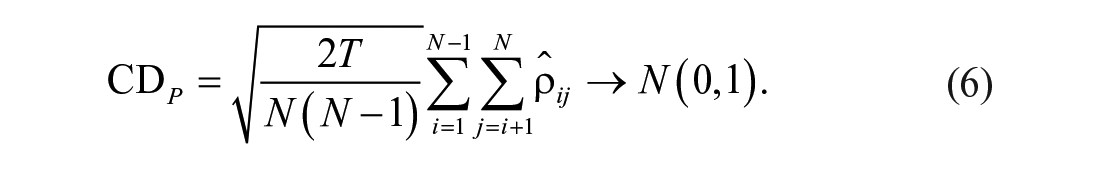
Thus, considering the pairwise correlation coefficients ${\widehat{\rho }}_{ij}$ among the cross-sectional residuals, the Cross-section Dependence (CD) test statistic as proposed by Pesaran is computed below as

$${\mathrm{CD}}_P=\sqrt{\frac{2T}{N\left(N-1\right)}}\sum _{i=1}^{N-1}\sum _{j=i+1}^N{\widehat{\rho }}_{ij}\to N\left(0,1\right).$$

(6)

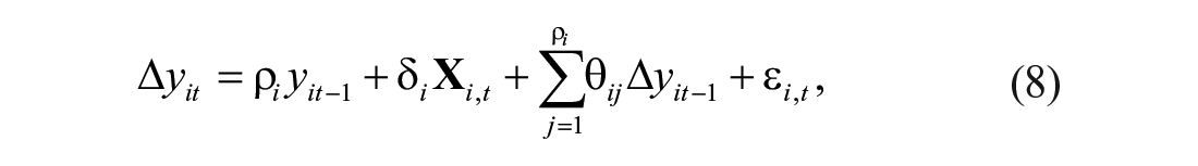
The study later analyzed the integration properties of the explanatory variables via unit root tests. The choice of a particular unit root test to be used will rely on the outcome of the cross-sectional reliance test. This is because there are two types of generations for the test of data stability. The first-generation unit root tests are more applicable to cross-sectional individuality, while the second-generation tests work perfectly for cross-sectional dependencies. Thus, due to the occurrence of cross-sectional independence among residual terms within all cross-sections with reference to Table 4, the study will employ first generation panel unit root tests. In testing the presence of unit root among the analyzed variables, the following equation will be used:

$$\mathrm{\Delta }{y}_{it}={\mathrm{\rho }}_i{y}_{it-1}+{\delta }_i{\mathbf{X}}_{i,t}+{\epsilon }_{i,t},$$

(7)

where $i=1,2,\dots ,N$ for each firm in the panel; $t=1,2\dots ,T$ stands for the time period; ${\mathbf{X}}_{i,t}$ denotes the vector of exogenous variables of the model which contains fixed effects or individual time trend; ${\mathrm{\rho }}_i$ symbolizes autoregressive coefficients; and ${\epsilon }_{i,t}$ is the error term of stationary sequence. Specifically, $y_{it}$ is considered to be weak in stationary trend if ${\mathrm{\rho }}_i<1,$ otherwise if ${\mathrm{\rho }}_i=1,$ $y_{it}$ is said to have a unit root. Due to autocorrelation that may occur in Equation 7, Levin et al. (2002) developed a higher order differential time-delay term similar to the Augmented Dickey–Fuller (ADF) test in the form

$$\mathrm{\Delta }{y}_{it}={\mathrm{\rho }}_i{y}_{it-1}+{\delta }_i{\mathbf{X}}_{i,t}+\sum _{j=1}^{{\mathrm{\rho }}_i}{\theta }_{ij}\mathrm{\Delta }{y}_{it-1}+{\epsilon }_{i,t},$$

(8)

where ${\mathrm{\rho }}_i$ represents number of lags in the regression and ${\epsilon }_{i,t}$ in this case becomes the white noise. Furthermore, Im et al. (2003) specified a t-bar statistic as the mean of the individual ADF statistic in the form

$$\overline{t}=\frac{1}{N}\sum _{i=1}^N{t}_{{\mathrm{\rho }}_i},$$

(9)

where $t_{{\mathrm{\rho }}_i}$ signifies the individual t statistic to test the null hypothesis of no stationarity. Generally, the t-bar statistic is distributed with respect to the null hypothesis where critical values for given values of N and T are provided by Im et al. (2003). The Levin, Lin, and Chu (LL & C) unit root test assumes that ${\mathrm{\rho }}_i=\mathrm{\rho },$ meaning all cross-sectional units are non-stationary whereas Fisher-ADF test together with Phillips–Perron–Fisher (PP-Fisher) test permit ${\mathrm{\rho }}_i$ to vary across different cross-sections.

If the outcome of the unit root tests establishes that the variables are integrated at the same order, then the study will move on to examine whether the variables are co-integrated or not. The Pedroni (2004) test and the Kao (1999) test for co-integration will be adopted for this study. These tests will be employed because they take into consideration cross-sectional independence with individual effects as evidenced in Table 4. The Pedroni panel co-integration test is built on the regression model in Equation 10 as follows:

$$y_{it}={\mathrm{\alpha }}_i+{\delta }_{i}t+{\mathrm{\beta }}_{1i}{x}_{1i,t}+{\mathrm{\beta }}_{2i}{x}_{2i,t}+\cdots +{\mathrm{\beta }}_{mi}{x}_{mi,t}+{\epsilon }_{it},$$

(10)

where ${\mathrm{\alpha }}_i$ and ${\mathrm{\beta }}_{ij}$ are the intercepts and slope coefficients that can vary across cross-sections, $t=1,\dots ,T,$ $i=1,\dots ,N,$ $m=1,\dots ,M;$ $x$ and $y$ are assumed to be integrated of the same order (I(1)). The null hypothesis of no co-integration of the Pedroni panel co-integration test is determined with respect to the error term $({\epsilon }_{it})$ which is expressed as

$${\epsilon }_{it}={\mathrm{\rho }}_i{\epsilon }_{it-1}+{\mathrm{\mu }}_{it}.$$

(11)

The alternative hypothesis, on the contrary, includes the homogeneous hypothesis $({\mathrm{H}}_A:{\mathrm{\rho }}_i=\mathrm{\rho }<1)$ for all individual series for the within-dimension test and heterogeneous alterative $({\mathrm{H}}_A:{\mathrm{\rho }}_i<1)$ also for all individual series for between-dimension test. Aside the aforementioned panel co-integration test, the Kao (1999) panel co-integration test generally depends on the ADF statistic for which the error terms are obtained by using the regression

$$y_{it}={\mathrm{\alpha }}_i+\mathrm{\beta }{x}_{it}+{\epsilon }_{it},$$

(12)

where the ADF statistic is computed as

$$\mathrm{ADF}=\frac{t_{\overline{p}}+\frac{\sqrt{6N{\widehat{\sigma }}_{ov}}}{2{\widehat{\sigma }}_{ov}}}{{\left(\frac{{\widehat{\sigma }}_{ov}^2}{2{\widehat{\sigma }}_{ov}^2}+\frac{3{\widehat{\sigma }}_{ov}^2}{10{\widehat{\sigma }}_{ov}^2}\right)}^{\frac{1}{2}}},$$

(13)

where ${\widehat{\sigma }}_v^2={\widehat{\sigma }}_u^2-{\widehat{\sigma }}_{u\epsilon }^2{\sigma }_{\epsilon }^{-2}$ is the estimates variance, ${\widehat{\sigma }}_{ov}^2={\widehat{\sigma }}_{ou}^2-{\widehat{\sigma }}_{ou\epsilon }^2{\sigma }_{o\epsilon }^{-2}$ represents the long-run covariance, and $t_{\overline{p}}$ denotes the t statistic of the ADF regression. The Koa test also tests the null hypothesis of no co-integration among variables in a cross-sectional data. Estimation of the long-term association between the variables can only be conducted through the fixed or random effects estimators if and only if both the Pedroni and Koa tests prove that the variables are co-integrated.

Finally, results of causality in this article will be documented by making use of Engle and Granger (1987) causality test. As documented by numerous studies, the affirmation of structural long-run relationship further gives the indication that there exist causalities among analyzed variables. The study thus applies Engle and Granger causality test to examine the causal relationship between the study variables. The models based on the Engle and Granger causality test employed in this study to examine causal liaison amid the variables are given as follows:

$$y_{it}={\mathrm{\alpha }}_o+\sum _{i=1}^m{\mathrm{\alpha }}_i{y}_{t-i}+\sum _{i=1}^m{\mathrm{\beta }}_i{x}_{t-i}+{\epsilon }_{it},$$

(14)

$$x_{it}={\mathrm{\alpha }}_o+\sum _{i=1}^m{\mathrm{\alpha }}_j{y}_{t-j}+\sum _{i=1}^m{\mathrm{\beta }}_j{x}_{t-j}+{\epsilon }_{it}.$$

(15)

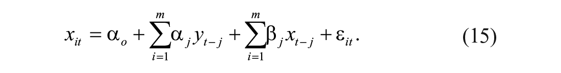
The null hypothesis of the Granger causality test demonstrates that X does not Granger cause Y and is expressed in Equation 16 as

$${\mathrm{H}}_O:{\mathrm{\beta }}_i=0,i=1,2,\dots ,n.$$

(16)

Conclusion can therefore be drawn that X Granger causes Y if and only if Equation 16 is rejected. In the same manner, another hypothesis test can be conducted to determine whether Y Granger causes X using Equation 17 which is expressed hypothetically as

$${\mathrm{H}}_O:{\mathrm{\beta }}_j=0,j=1,2,\dots ,n.$$

(17)

Theoretical Framework

Empirically, the analysis is ensued in a step-by-step manner and also summarily illustrated in Figure 1:

Step 1: Cross-sectional reliance test

The first step of the empirical analysis process is to undertake a cross-sectional reliance test. The test will decide the methods to be utilized to perform the unit root and co-integration tests.

Step 2: Panel unit root test

The study will then proceed to test for the stability or instability of the studied variables through unit root tests. If the variables are found to be stable, then their attributes will be examined through regression analysis. However, if the variables do not attain stability at any order, then the process of analysis will be terminated. When the variables attain stability (specifically after the first difference), the Autoregressive Moving Average analysis technique will be employed for the analysis of a univariate model, and a co-integration test will be conducted in the case of a multivariate model.

Step 3: Panel co-integration test

If stability of the variables is uncovered per the outcome of the unit root tests, their co-integration properties will be explored through the Pedroni and Kao panel co-integration tests. If the tests uncover no co-integration among the variables, then further analysis of the series will not be possible. However, if the existence of co-integration is discovered among the variables, then the analysis process will continue to the next stage.

Step 4: Model form determination

If the variables are found to be co-integrated, the Hausman test will be used to determine the model form (random effect or fixed effect model). Based on the determined model form, the study’s model will be estimated to examine the elasticities of the response variable with respect to the explanatory variables.

Step 5: Serial correlation and heteroscedasticity tests

After estimating the study’s model, the Wooldridge (2015) serial correlation test and the Breusch–Pagan heteroscedasticity test will be conducted to authenticate the reliability of the established working model.

Step 6: Granger causality test

The Granger causality test will finally be conducted to explore the causative link between the variables under study. The direction of the association between the variables will help provide implications for policy makers.

Figure 1.

Framework for examining the liaison amid liquidity and firms’ financial performance.

Data Source and Summary Statistics

All the non-financial establishments quoted on the GSE formed the study’s population. Currently, the entire number of quoted firms on the stock market total 41. Out of this figure, non-financial firms account for 28 representing 68.29% of the entire figure of listed firms. Because the study wanted to use a balanced data, the purposive or selective sampling method was employed to make a sample out of the total population. The number of years in existence, technical suspension, unaudited financial records, incomplete financial statements, and the presentation of annual reports in foreign currencies other than that of the currency of Ghana (because of the non-stability of the Ghana Cedi to major foreign currencies) were the factors or filters that were considered during the sampling process. Firms that failed in any of the above filters or factors did not form part of the study’s sample. In all, 13 firms were rejected as they failed in one or more of the factors that were considered for the sampling. The sample therefore totaled 15 representing 53.57% of the target population or 36.59% of the total number of listed firms. Panel data sourced from the audited and published annual reports of the carefully chosen businesses for the period 2008–2017 was then used for the study. Table 1 presents a summary of the study variables and how they were measured.

Table 1.

Measurement of Study Variables.

Variable	Proxy	Measurement
ROE	Financial performance	Net income / total equity
CR	Liquidity	Total current assets / total current liabilities
CFR	Liquidity	Net cash flows from op. / total current liabilities
SIZE	Control variable	Natural log of total assets
GRO	Control variable	(Size t – Sizet-1) / Sizet-1
EFF	Control variable	Gross revenue / total assets
TAN	Control variable	Total tangible assets / total assets

Note. ROE = Return on Equity; CR = Current Ratio; CFR = Cash Flow Ratio; SIZE = Size; GRO = Growth; EFF = Efficiency; TAN = Tangibility.

Descriptive statistics on the study variables are displayed in Table 2. From the table, lnROE had an average value of –1.624734 and a standard deviation of 1.069139. This is an indication that data values of lnROE were a bit much dispersed from the mean. The distribution for lnROE ranged between –4.892852 and 1.510214, while the skewness coefficient of –0.3250714 indicates that the data values of lnROE were negatively skewed. The kurtosis value of 3.851733 (excess [K] = 3.851733 – 3.0 = 0.851733) shows that, the distribution for lnROE was not normally distributed. Also, lnCR had a mean value of –0.0142636, a maximum value of 2.039257, and a minimum value of –3.329807, resulting in a range of 5.369064. The natural logarithm of CR had a standard deviation of 0.8041956. This implies, dispersions or deviations around the mean lnCR was 0. 8041956. The skewness value of –0.9966623 for lnCR means the lnCR distribution was highly positively skewed. The kurtosis coefficient of 7.230972 (excess [K] = 7.230972 – 3.0= 4.230972) is an indication that the lnCR distribution was not normally distributed.

Table 2.

Descriptive Statistics on Study Variables.

Variable	M	SD	Variance	Minimum	Maximum	Range	Skewness	Kurtosis
lnROE	−1.624734	1.069139	1.143059	−4.892852	1.510214	6.403066	−0.3250714	3.851733
lnCR	−0.0142636	0.8041956	0.6467306	−3.329807	2.039257	5.369064	−0.9966623	7.230972
lnCFR	−1.560014	1.309895	1.715825	−5.521461	1.482491	7.003952	−0.4645787	3.619178
lnSIZE	−2.17978	1.703942	2.903417	−6.319969	1.562724	7.882693	−0.4407403	3.048133
lnGRO	−2.02005	1.418711	2.01274	−6.119298	0.9269537	7.046252	−0.2837305	3.021976
lnEFF	0.1993689	0.7575628	0.5739015	−1.65653	2.069846	3.726376	0.3717903	2.58801
lnTAN	−0.1681108	0.2957183	0.0874493	−2.092324	0.0000	2.092324	−3.093788	16.33707

Note. ROE = Return on Equity; CR = Current Ratio; CFR = Cash Flow Ratio; SIZE = Size; GRO = Growth; EFF = Efficiency; TAN = Tangibility.

LnCFR of the sampled firms had a mean figure of –1.560014, a maximum figure of 1.482491 and a minimum figure of –5.521461, resulting in a range of 7.003952. The standard deviation of lnCFR of 1.309895 indicates that the data values of lnCFR were a bit widely dispersed from the mean. The natural logarithm of CFR had a skewness value of –0.4645787, which is an indication that, the distribution for lnCFR was negatively skewed. The kurtosis value of 3.619178 (excess [K] = 3.619178 – 3.0 = 0.619178) for lnCFR implies its distribution was of abnormal shape. The mean lnSIZE of the quoted establishments was –2.17978 with a standard deviation of 1.703942 and a variance of 2.903417. The data values of lnSIZE ranged from –6.319969 to 1.562724, and had an adversely skewed distribution with a coefficient of –0.4407403. The kurtosis value of 3.048133 (excess [K] = 3.048133 – 3.0 = 0.048133) shows that the lnSIZE distribution was of lower, less distinct peak (platykurtic).

LnGRO had an average value of –2.02005 and a standard deviation of 1.418711. This implies, deviances from the mean lnGRO was 1.418711. The data values of lnGRO ranged from –6.119298 to 0.9269537 and had a negatively skewed distribution with a coefficient of –0.2837305. The kurtosis coefficient of 3.021976 (excess [K] = 3.021976 – 3.0 = 0.021976) implies the lnGRO distribution was not normally distributed. Furthermore, lnEFF had a mean value of 0.1993689 and a standard deviation of 0.7575628. LnEFF of the sampled firms ranged from –1.65653 to 2.069846, and had a favorably skewed distribution with a coefficient of 0.3717903. The figure 2.58801 as the kurtosis statistic of lnEFF indicates that the lnEFF distribution was abnormally distributed. Finally, lnTAN had a mean value of –0.1681108 and a standard deviation of 0.2957183. The data for lnTAN ranged between –2.092324 and 0.0000, and had an inversely skewed distribution with a coefficient of –3.093788. The kurtosis value of 16.33707 (excess [K] = 16.33707 – 3.0 = 13.33707) implies the lnTAN distribution was of abnormal shape.

Because multi-collinearity could lead to extreme confidence intervals and less dependable probability values resulting in skewed or misleading inferences (Gujarati & Porter, 2009), the researchers decided to find out whether the explanatory variables were highly correlated or not. Multi-collinearity was detected through the Variance Inflation Factor (VIF) or the degree of tolerance (1 / VIF) after running the OLS regression with lnROE as the response variable and lnCR, lnCFR, lnSIZE, lnGRO, lnEFF, and lnTAN as the explanatory variables. The rule of thumb was that, a variable with a VIF more than 5 (VIF > 5) or a degree of tolerance lower than 0.2 (1 / VIF < 0.2) was considered to be highly collinear with the other explanatory variables. From Table 3, the VIFs of lnCR, lnCFR, lnSIZE, lnEFF, lnTAN, and lnGRO with their respective degrees of tolerance (1 / VIF) indicated that the variables were not extremely related to each other (VIF < 5; 1 / VIF > 0.2). This implies, all the variables qualified to be used together in the study.

Table 3.

Multi-Collinearity Test Results.

Variable	VIF	1 / VIF
lnSIZE	2.99	0.334597
lnGRO	2.34	0.427603
lnCR	1.70	0.588000
lnCFR	1.36	0.736931
lnTAN	1.06	0.944088
lnEFF	1.06	0.944933
Mean VIF	1.75

Note. VIF = Variance Inflation Factor; SIZE = Size; GRO = Growth; CR = Current Ratio; CFR = Cash Flow Ratio; TAN = Tangibility; EFF = Efficiency.

Empirical Results

Cross-Sectional Dependence Test Results

The actual empirical analysis procedure began by testing for the existence or absence of cross-sectional reliance in the study’s model. Pesaran’s test for cross-sectional reliance was employed for that purpose, and from Table 4, the null hypothesis of cross-sectional independence could not be rejected.

Table 4.

Pesaran’s Residual Cross-Sectional Dependence Test Results.

Test method	Statistic	Probability
Pesaran CD	−1.075326	.2822

Panel Unit Root Test Results

Numerous time-dependent data used in econometric analysis are often non-stationary, meaning they have the tendency to either increase or decrease over time. According to Engle and Granger (1987), such data if used for regression analysis would lead to spurious conclusions or inferences. This assertion is supported by Hegwood and Papell (2007) who indicated that unit root leads to errant behavior due to the assumptions of analysis not being valid (for instance, t ratios will not follow a t distribution). Therefore, before undertaking a co-integration test to establish whether there existed a long-term association between the explained and the explanatory variables, it was imperative to examine the stability of the input variables. Because the Pesaran’s test uncovered cross-sectional independence in the panel, first-generation unit root tests like LL & C t test; Im, Pesaran, and Shin W-stat (IPS) test; Augmented Dickey–Fuller–Fisher (ADF-Fisher) test, and PP-Fisher test were employed for the unit root diagnosis. As displayed in Table 5, the studied variables were not stable at levels, hence the failure to reject the null hypothesis of non-stability. However, the study rejected the null hypothesis at first difference because the variables attained stability.

Table 5.

Panel Data Unit Root Test Results.

Order	Variable	LL & C	IPS	ADF-Fisher	PP-Fisher	Conclusion
Levels	lnCR	1.18662	2.14038	17.8163	17.1173	Non-stationary
		(.8823)	(.9838)	(.9614)	(.9711)
	lnCFR	−1.24993	−1.07209	39.0243	101.160	Non-stationary
		(.1057)	(.1418)	(.1252)	(.0000) ∗
	lnSIZE	−2.25540	−0.97888	35.8322	52.8237	Non-stationary
		(.1121)	(.1638)	(.2136)	(.0062) ∗
	lnGRO	−3.41923	−1.14210	40.1029	50.8057	Non-stationary
		(.0003) ∗	(.1267)	(.1029)	(.1012)
	lnEFF	−1.80491	−0.40027	33.7599	41.3694	Non-stationary
		(.0355) ∗∗	(.3445)	(.2905)	(.1089)
	lnTAN	3.35423	0.94782	29.8939	103.309	Non-stationary
		(.9996)	(.8284)	(.4711)	(.0000) ∗
First Difference	lnCR	−5.40703	−1.50942	43.2916	86.3826	Stationary
		(.0000) ∗	(.0656) ∗∗∗	(.0552) ∗∗∗	(.0000) ∗
	lnCFR	−8.46675	−4.78469	83.3502	231.993	Stationary
		(.0000) ∗	(.0000) ∗	(.0000) ∗	(.0000) ∗
	lnSIZE	−6.64808	−2.86557	61.4387	128.498	Stationary
		(.0000) ∗	(.0021) ∗	(.0006) ∗	(.0000) ∗
	lnGRO	−7.73034	−3.22512	66.1075	145.471	Stationary
		(.0000) ∗	(.0006) ∗	(.0002) ∗	(.0000) ∗
	lnEFF	−6.94934	−2.32722	55.5124	115.564	Stationary
		(.0000) ∗	(.0100) ∗	(.0031) ∗	(.0000) ∗
	lnTAN	0.14498	−1.80405	49.9291	219.624	Stationary
		(.5576)	(.0356) ∗∗	(.0126) ∗∗	(.0000) ∗

Note. Figures in parenthesis denote probabilities. LL & C = Levin, Lin, and Chu; IPS = Im, Pesaran and Shin W-stat; ADF-Fisher = Augmented Dickey–Fuller–Fisher; PP-Fisher = Phillips–Perron–Fisher; CR = Current Ratio; CFR = Cash Flow Ratio; SIZE = Size; GRO = Growth; EFF = Efficiency; TAN = Tangibility.

∗,∗∗,∗∗∗

signify rejection of the null hypothesis at 1%, 5%, and 10% significance levels, respectively.

Panel Co-Integration Test Results

Because all the variables were stationary at first difference, the researchers proceeded to establish whether the variables were co-integrated in the long run or not. Pedroni and Kao’s tests for co-integration were adopted for that purpose. Based on the outcome of four of Pedroni’s test statistics shown in Table 6, the null hypothesis of no co-integration among the variables was rejected. Kao’s test results displayed in Table 7 also supported this conclusion.

Table 6.

Pedroni’s Residual Co-Integration Test Results.

Test statistics	Value	Probability
Panel v-Statistic	−1.257451	.8957
Panel rho-Statistic	3.739192	.9999
Panel PP-Statistic	−4.618223	.0000 ∗
Panel ADF-Statistic	−4.338545	.0000 ∗
Group rho-Statistic	6.113388	1.0000
Group PP-Statistic	−6.423036	.0000 ∗
Group ADF-Statistic	−3.594718	.0002 ∗

Note. PP = Phillips–Perron; ADF = Augmented Dickey–Fuller.

∗

Denotes rejection of the null hypothesis at 1% significance level.

Table 7.

Kao’s Residual Co-Integration Test Results.

Test	t statistic	Probability
ADF	−2.054421	.0200 ∗∗
Residual variance	1.666430
HAC variance	0.318522

Note. ADF = Augmented Dickey–Fuller; HAC = Heteroscedasticity and Autocorrelation Consistent.

∗∗

Denotes rejection of the null hypothesis at 5% significance level.

Model Form Determination

The Durbin–Wu–Hausman test with the null hypothesis of the random effects model which was preferable to that of the fixed effects model (Durbin, 1954; Hausman, 1978; Wu, 1973) was adopted for the study’s model form determination. From Table 8, results of the specification test showed a χ² of 3.088725 with a probability of .7976. The outcome was statistically insignificant at the chosen alpha (α) levels. The study therefore rejected the fixed effects model in favor of the random effects model.

Table 8.

Hausman Test Results.

Test summary	χ2 statistic		χ2 df	Probability
Cross-section random	3.088725		6	.7976
Cross-section random effects test comparisons
Variable	Fixed	Random	Var(Diff.)	Probability
lnCR	−0.305028	−0.322310	0.008167	.8483
lnCFR	0.026455	0.030752	0.000573	.8575
lnSIZE	0.089760	0.085834	0.000179	.7695
lnGRO	−0.060423	−0.038753	0.000228	.1517
lnEFF	−0.048014	0.109606	0.020357	.2693
lnTAN	0.057316	0.030525	0.004782	.6985

Note. CR = Current Ratio; CFR = Cash Flow Ratio; SIZE = Size; GRO = Growth; EFF = Efficiency; TAN = Tangibility.

Model Estimation

From the study’s findings (see, Table 9), lnCR had a significantly negative impact on the firm’s lnROE (β = –.3223098, p = .045). The outcome is an indication that, on the average, when all other variables were held stationary, a unit increase in lnCR led to –.3223098 decrease in lnROE. This finding was consistent with that of Kimondo et al. (2016), Mulyana and Zuraida (2018), Ali et al. (2018), Kanga and Achoki (2017), and Ali and Bilal (2018) whose studies uncovered liquidity as a significant predictor of firms’ viability. The finding was however not consistent with Mutwiri (2015), Jepkemoi (2017), Syed (2015), and Opoku (2015) whose studies found statistically insignificant influence of liquidity on firms’ financial performance. The finding was also not consistent with the priori expectation of the study that β₁ > 0. LnCR having a significantly adverse influence on lnROE might be that the firms were investing too much in current assets like inventories of which they were finding it very difficult to turnover. As inventories are been kept too long in firms, they attract high storage costs and other carrying expenses. This adversely affect the viability of firms. Per the findings on lnCR, the study’s hypothesis that liquidity had a significant effect on the firms’ financial performance could not be rejected.

Table 9.

Estimated Results of the Variable Parameter Model With Random Effects.

Variable	Coefficient (β)	Robust SE	z statistic	p > |z|	Confidence interval
lnCR	−.3223098	0.1606809	−2.01	0.045 ∗∗	[–0.6372385, –0.007381]
lnCFR	.0307524	0.0744022	0.41	0.679	[–0.1150733, 0.1765782]
lnSIZE	.0858339	0.079618	1.08	0.281	[–0.0702145, 0.2418823]
lnGRO	−.0387533	0.0843414	−0.46	0.646	[–0.2040595, 0.1265529]
lnEFF	.1096064	0.1698911	0.65	0.519	[–0.2233739, 0.4425868]
lnTAN	.0305249	0.2786361	0.11	0.913	[–0.5155919, 0.5766417]
CONS	−1.489262	0.251764	−5.92	0.000	[–1.98271, –0.9958131]
R2:			Wald χ2(6)	5.11
Within		.0228	Prob > χ2	.5301
Between		.2083	Number of observations	150
Overall		.0781	Number of groups	15

Note. CR = Current Ratio; CFR = Cash Flow Ratio; SIZE = Size; GRO = Growth; EFF = Efficiency; TAN = Tangibility.

∗∗

Denotes significance at the 5% significance level.

Also, lnCFR had an insignificantly positive impact on lnROE (β = .0307524, p = .679). The finding implies, on the average, when all other variables were held constant, changes in lnCFR did not lead to any vital increase in the firms’ financial performance. This outcome supported that of Ayako et al. (2015), Batchimeg (2017), and Ashutosh and Gurpreet (2018), whose studies discovered liquidity as an insignificant predictor of firms’ viability. The finding though insignificant, agreed with the study’s estimation that β₂ > 0. The finding did not agree with Isik (2017), Kung’u (2017), Saripalle (2018), Mohd and Asif (2018), and A. Mehmet and Mehmet (2018), whose studies uncovered liquidity as a significant determinant of firms’ profitability. LnCFR having an insignificantly positive influence on lnROE might be that the firms were not effectively managing their cash flow strategies to generate more funds. For instance, the firms might be operating with longer receivables collection period and longer CCCs among others. Per the findings on lnCFR, the study’s hypothesis that liquidity had a significant effect on the firms’ financial performance could not be accepted.

Furthermore, lnSIZE of the sampled firms positively affected lnROE and the effect was statistically insignificant (β = .0858339, p = .281). The outcome signifies that, on the average, when all other factors were held fixed, a unit increase in lnSIZE did not have any material influence on the firms’ financial performance. This finding was consistent with Sivathaasan et al. (2013) whose research on 11 publicly traded manufacturing firms in Sri Lanka found size as an insignificant predictor of the firms’ financial performance. The finding though insignificant supported the study’s projection that β₃ > 0. The finding was however not consistent with Shehryar (2017) whose study on 50 quoted firms on Borsa Italiana for the period 2007–2015 revealed size as a significant predictor of firms’ profitability. In addition, lnGRO had an insignificantly negative effect on the firms’ lnROE (β = –.0387533, p = .646). This outcome denotes that, on the average, when all other factors were held fixed, an increase in lnGRO did not lead to any significant decrease in the firms’ lnROE. The finding was in tandem with Ngoc et al. (2017) whose research on 739 very large and large quoted establishments in London for the period 2006–2015 discovered growth as an insignificant determinant of the firms’ profitability. The finding was however not consistent with Ropafadzai (2017) whose study on 52 quoted industrial businesses on the Johannesburg Stock Exchange (JSE) in South Africa established a significantly positive influence of growth on the firms’ profitability. The finding though trivial, did not agree with the study’s estimation that β₄ > 0.

The study also revealed an insignificantly positive influence of lnEFF on the firms’ lnROE (β = .1096064, p = .519). This outcome is an indication that, on the average, when all other variables were held constant, changes in lnEFF did not lead to any vital increase in the firms’ lnROE. The finding was consistent with that of I. Mehmet and Nuri (2015) whose research on quoted paper and paper products businesses in Turkey for the period 2011–2001 to 2014–2009, found management efficiency as an insignificant predictor of the firms’ profitability. The finding though immaterial, supported the study’s prediction that β₅ > 0. The finding was however not consistent with Cuong et al. (2018) whose study on 30 listed construction-material establishments in Vietnam uncovered operational efficiency as a significant predictor of the firms’ financial performance.

Finally, lnTAN had an insignificantly positive effect on lnROE (β = .0305249, p = .913). This outcome means, when all other factors were held constant, a unit increase in lnTAN did not lead to any significant increase in the firms’ lnROE. The finding was in line with Nikhil et al. (2015) whose research on 13 insurance establishments in India uncovered tangibility as an insignificant determinant of the firms’ profitability. Although very trivial, the finding supported the study’s estimation that β₆ > 0. The finding was however not consistent with Kristina and Dejan (2017) whose study on the agricultural industry in Hungary, Romania, Bosnia and Herzegovina, and Serbia found tangibility as a significant predictor of the firms’ profitability.

The overall R² value of .0781 implies the liquidity proxies together with the control variables accounted for only 7.81% of the variances in lnROE, while 92.19% (100 – 7.81) of the variances was explained by other inherent variabilities. The overall R² value was statistically insignificant, implying, the goodness of fit of the model was very low. This is substantiated by the Wald χ² value of 5.11 which was statistically immaterial with a probability of .5301. The Wald χ² value with its corresponding probability implies lnCR, lnCFR, lnSIZE, lnGRO, lnEFF, and lnTAN did not significantly account for the variations in lnROE, or had a combined insignificant effect on the firms’ financial performance as measured by lnROE.

Heteroscedasticity and Serial Correlation Tests Results

The study examined the validity of the established model by testing for the presence or absence of heteroscedasticity and serial correlation in the working model. From the Breusch and Pagan (1979) heteroscedasticity test results, the null hypothesis of homoscedasticity among the fitted values of the model could not be rejected. Also from the Wooldridge’s (2015) serial correlation test results, the null hypothesis of no serial correlation in the panel could not be rejected. Findings from these two tests signposts that the established panel data model was valid. Table 10 therefore outlines the results based on the heteroscedasticity and serial correlation tests.

Table 10.

Heteroscedasticity and Serial Correlation Test Results.

Test type	Test method	Test value	Probability
Heteroscedasticity test	Breusch and Pagan test	0.48	.4898
Serial correlation test	Wooldridge test	0.016	.9020

Granger Causality Test Results

The Engle and Granger (1987) test for causality was used to establish the causal connections between lnCR, lnCFR, lnSIZE, lnGRO, lnEFF, lnTAN, and lnROE. From the results depicted in Table 11, the following inferences were made:

1. There was a bidirectional causal relationship between lnCR and lnROE. This implies an increase or decrease in lnCR led to a significant increase or decrease in lnROE and vice-versa. Per this outcome, the study’s hypothesis that liquidity had a causal affiliation with the firms’ financial performance could not be rejected. This finding supported that of Anowar (2016) whose research on 40 listed firms on the DSE affirmed a bidirectional causality between liquidity and the firms’ profitability. The finding also supported that of Reis and Aydin (2014) who established a feedback causality between liquidity and the viability of firms operating under the BIST 100 index of Turkey. This finding was further consistent with Nyamiobo et al. (2018) whose study on some quoted firms in Kenya confirmed a noteworthy link between liquidity and the firms’ viability. The finding was also consistent with Swagatika and Ajaya (2018) whose research on some Indian manufacturing firms discovered a significant connection between liquidity and the firms’ profitability. The finding was however not consistent with Z. R. Mohammed et al. (2015) whose study on 99 listed non-financial firms in Saudi Arabia discovered an insignificant association between liquidity and the firms’ profitability. The finding was also not consistent with Ayako et al. (2015) whose research on 41 quoted businesses in Kenya established no significant association between liquidity and the firms’ profitability. Linking the causal relationship between lnCR and lnROE to the significantly negative influence of lnCR on the firms’ viability obtained from the study’s regression estimates, one may conclude that the firms were not investing their liquid resources into investments that were capable of earning them positive returns. The reason might also be that, the entities were not deploying effective internal control systems that could strengthen the liquidity fundamentals of the firms. Especially, if the firms were operating with weak controls on cash management.

2. There was no causal relationship between lnCFR and lnROE. Based on this finding, the study’s hypothesis that liquidity had a causal affiliation with the firms’ financial performance could not be accepted. This finding agreed with Dabiri et al. (2017) whose research on five institutions in the United Kingdom found no causality between liquidity and the firms’ profitability. The finding also agreed with Osadune and Ibenta (2018) whose study on some selected firms in Nigeria disclosed the absence of a causality between liquidity and the firms’ financial performance. The finding further supported that of Maina (2017) whose research on 42 establishments in Kenya uncovered no causality between liquidity and the firms’ viability. The finding also agreed with Batchimeg (2017) whose study on 100 listed JSC in Mongolia found an insignificant affiliation between liquidity and the firms’ profitability. The finding finally supported that of Ashutosh and Gurpreet (2018) whose research on sugar mills in Punjab India discovered an insignificant association between liquidity and the profitability of private sugar mills in the sugar industry. The finding did not agree with Kanga and Achoki (2017), Ejike and Agha (2018), Banafa et al. (2015), and Kaysher and Rowshonara (2016) whose studies found vital connections between liquidity and firms’ viability. The non-existence of a causal relationship between liquidity and the firms’ financial-related issues might well be that the firms were not boosting their expansion activities through product diversification strategies. The firms could enlarge their scope based on these strategies, thereby advancing their revenue base and subsequently their liquidity positions. The reason might also be that the firms were operating with a low receivables turnover ratio and an increasing average period of inventory. All these have repercussions on the firms’ ability to generate more cash flows.

3. Furthermore, lnSIZE had no causal relationship with the firms’ lnROE. This finding was consistent with Sivathaasan et al. (2013) whose research on 11 publicly traded manufacturing firms in Sri Lanka found no significant link between size and the firms’ financial performance. The finding also agreed with Avdalović (2018) and Odusanya et al. (2018) whose studies uncovered insignificant affiliations between size and firms’ financial performance. The finding was not consistent with Kamran et al. (2017) whose research on some listed firms in Pakistan found a material link between size and the firms’ profitability. The finding was also not consistent with Andow et al. (2017) and Shehryar (2017) whose studies discovered significant interactions between size and firms’ viability.

4. There was also no causal affiliation between lnGRO and lnROE. This finding was in tandem with Khan et al. (2018) whose research on five listed telecommunication companies in India found no significant connection between growth and the firms’ financial performance. The finding also supported Meseret and Getahun (2017) and Vuong (2017) whose studies uncovered no material association between growth and firms’ viability. The finding was inconsistent with Niar et al. (2018) whose research on 55 quoted manufacturing establishments in Indonesia uncovered a significant interaction between growth and the firms’ viability. The finding was also inconsistent with Ngoc et al. (2017) and Ropafadzai (2017) whose studies established a significant link between growth and firms’ profitability.

5. The study also discovered no causal relationship between lnEFF and lnROE. This finding supported that of Gichuhi (2016) whose research on 36 quoted corporations in Kenya uncovered no significant association between operational efficiency and the firms’ profitability. The finding also agreed with I. Mehmet and Nuri (2015) and M. K. Mohammed et al. (2016) whose studies found an insignificant interplay between operational efficiency and firms’ economic health. The finding did not agree with Cuong et al. (2018) whose panel study on 30 listed construction-material establishments in Vietnam discovered a significant link between efficiency and the viability of the entities. The finding also contrasted that of Al Shahrani and Zhengge (2016) and Alemu (2015) whose research revealed insignificant connections between operational efficiency and firms’ financial performance.

6. There was finally no causal relationship between lnTAN and lnROE. This finding was in line with Navleen and Jasmindeep (2016) whose study on the automobile industry of India found an insignificant link between tangibility and the firms’ profitability. The finding was also in tandem with Nikhil et al. (2015) and Demis (2016) whose studies discovered an insignificant nexus among tangibility and firms’ profitability. The finding was however not consistent with Al-Jafari and Al Samman (2015) whose research on 17 quoted industrial firms in Oman established a relevant connection between tangibility and the firms’ profitability. The finding was also at variance with Kristina and Dejan (2017) and Birhan (2017) whose studies uncovered significant associations between tangibility and firms’ financial performance.

Table 11.

Granger Causality Test Results.

Null hypothesis	F statistic	Probability
LnCR does not Granger Cause lnROE	2.90541	.0906 ∗∗∗
LnROE does not Granger Cause lnCR	4.37308	.0384 ∗∗
LnCFR does not Granger Cause lnROE	1.34706	.2479
LnROE does not Granger Cause lnCFR	0.49370	.4835
LnSIZE does not Granger Cause lnROE	0.00155	.9687
LnROE does not Granger Cause lnSIZE	0.57026	.4515
LnGRO does not Granger Cause lnROE	1.01080	.3166
LnROE does not Granger Cause lnGRO	0.00908	.9242
LnEFF does not Granger Cause lnROE	1.94676	.1653
LnROE does not Granger Cause lnEFF	0.29954	.5851
LnTAN does not Granger Cause lnROE	0.01119	.9159
LnROE does not Granger Cause lnTAN	0.49472	.4831

Note. CR = Current Ratio; ROE = Return on Equity; CFR = Cash Flow Ratio; SIZE = Size; GRO = Growth; EFF = Efficiency; TAN = Tangibility.

∗∗,∗∗∗

Denote rejection of the null hypothesis at the 5% and 10% significance levels, respectively.

Conclusions and Limitations

This study examined the nexus between liquidity and the viability of quoted non-financial establishments in Ghana. Before the actual empirical analysis procedure began, the researchers conducted a multi-collinearity test to find out if the explanatory variables were highly correlated or not. From the VIF and tolerance test findings, the explanatory variables were not extremely correlated to each other, signifying that all the variables were fit enough to be used together in the study. The actual analysis process began by testing for cross-sectional reliance or independence in the panel. From the test’s findings, no cross-sectional reliance existed in the panel. Stability or instability of the variables was then examined through unit root tests. From the tests’ results, all the variables were unstable at levels but became stable at first difference. Co-integration attributes of the variables were then explored through the Pedroni and Kao’s tests. From the tests’ results, all the variables were co-integrated in the long run. The Durbin–Wu–Hausman test was then employed for this study’s model form determination. The test’s outcome was statistically insignificant at the three chosen alpha (α) levels. Based on this, the random effects model was the most appropriate. After the model form had been determined, the effects of the individual input variables on the firms’ ROE was examined through the analysis of their coefficients (β).

From the study’s random effects GLS regression estimates, liquidity proxied by CR had a significantly negative influence on the firms’ ROE. Therefore, the study’s hypothesis that liquidity had a material effect on the firms’ viability could not be rejected. It was also uncovered that liquidity surrogated by the CFR had an insignificantly positive influence on the firms’ ROE. Per this outcome, the study’s hypothesis that liquidity had a significant effect on the firms’ financial performance could not be accepted. It was further uncovered that control variables SIZE, GRO, EFF, and TAN had a trivial effect on the firms’ ROE. Finally, CR, CFR, SIZE, GRO, EFF, and TAN had no joint significant influence on the firms’ viability. The study then progressed to examine the validity of the estimated model by testing for the presence or absence of heteroscedasticity and serial correlation in the working model, through the Breusch and Pagan (1979) heteroscedasticity test and the Wooldridge’s (2015) serial correlation test. From the tests’ results, there was no heteroscedasticity and serial correlation in the model. This signified that the model was valid.

The Engle and Granger (1987) test for causality was finally employed to test for the causal connections between the variables understudy. From the test’s results, there was a bidirectional causal relationship between CR and ROE. Therefore, the study’s hypothesis that liquidity had a causal relationship with the firms’ financial performance could not be rejected. However, there was no causal relationship between CFR and ROE. Per this finding, the study’s hypothesis that liquidity had a causal relationship with the firms’ financial performance could not be accepted. There were finally no causal affiliations between SIZE, GRO, EFF, TAN, and ROE. Based on the findings, the following recommendations are proposed:

1. To ensure continuous survival and success, the firms should not play with the issue of liquidity management. The entities are required to keep an optimal liquidity level that will be capable of performing the “twin” role of meeting their financial obligations and at the same time maximizing their shareholders’ wealth. This optimal liquidity level could be obtained if the establishments are to meet the standards set by the GSE. Adhering to these standards will aid the firms to bring down the cases of financial drought. In other words, the firms should keep an adequate level of liquidity that will not portend their going concern status, and yet allow them to make ample returns on their investments. Thus, the firms should strike a balance (trade-off) between their liquidity and profitability.

2. The study further recommends for the deployment of effective internal control systems that could strengthen the liquidity fundamentals of the firms. More specifically, tighter systems or controls on cash management should be rooted for.

3. The establishments should also consider seeking for professional guidance toward the adoption of asset-liability management policies. By so doing, personnel in charge of finances in the firms would gain in-depth knowledge on the determination of liquidity levels that would not be of disadvantage to the firms.

4. In order for the firms to increase their profitability, there is also the need for them to increase their size in the aspects of customer base, net assets, sales volume, and market share. The firms increasing their size will not only boost them in terms of profitability, but will aid them to gain competitive advantage over others. The firms will further gain economy of scale when they increase their sizes. Economy of scale gained from increased firm size performs a vital function in predicting firms’ viability. Therefore, the firms should not only target local markets but should tactically increase their activities to other terrestrial markets in the globe. Thus, the firms establishing various branches at different locations is tactically paramount if they are to maximize returns on their investments.

5. The firms’ receivables turnover ratio ought to be well observed and followed to find out if a path is evolving overtime. This ratio evaluates firms’ efficacy in tracking their receivables or cash owed by clients. A high receivables turnover proportion demonstrates that the firms are effective in collecting their obligations and that they have a high extent of quality clients that pay their obligations rapidly. On the contrary, a low receivables turnover ratio may be due to the firms having some destitute collection strategies, appalling credit approaches, or clients that are not fiscally or financially sound.

6. Finally, the firms should track and reduce their average period of inventory to help improve cash flows. This ratio shows how long it takes firms to sell their current inventory. In other words, the ratio indicates how long inventory sits on firms’ shelves and remain unsold. This ratio is important to firms because it shows how inventory turnover changes overtime. The ratio allows authorities in firms to be abreast with procurement events and sales movements so as to curtail carrying costs associated with inventory. The ratio also helps management to know the products that are moving very quickly and those that are remaining stagnant. Thus, it shows firms’ efficiency in converting goods into sales. An increasing average inventory period depicts that it takes too long for firms to sell their goods, while the contrary implies, firms’ products are moving at a faster rate.

This study cannot be concluded without touching on its limitations. The study was confined to a sample of 15 firms because of data constraints. For instance, as of December 31, 2017, firms like Intraveneous Infusions Ltd, Meridian Marshalls Holdings, Samba Foods Ltd, Digicut Production and Advertising Ltd, and the Hords had just been listed some few years on the Ghana bourse. Also, not all the firms were actively operational during the study period. For instance, Pioneer Kitchenware Ltd and Cocoa Processing Company Ltd had been suspended in August 2017 for failing to meet “continuing listing obligations” of the stock market, in spite of several promptings to do so. Among their breaches were failure to submit financial reports for some number of years; the non-payment of annual listing fees; and failure to conduct annual general meetings (AGMs). Furthermore, firms like Golden Star Resources and Ayrton Drugs Manufacturing Ltd among others did not have their complete annual reports on the Ghana stock market as of December 31, 2017. These limitations among others made it impossible for some of the firms to contribute a fully balanced data for the study. Hence, the adoption of the purposive sampling technique to select the firms that had their data up-to-date.

Also, this study could not be generalized to include other body corporates in Africa because regulations that govern the operations of those businesses are not the same as the ones in Ghana. For instance, the minimum capital requirements for listed firms in Ghana differ from that of Nigeria, Senegal, Ivory Coast, and Togo among others. Furthermore, factors that affect businesses in other African countries are not the same as those in Ghana. For instance, high interest rates, inflation, the rampant fall of the Ghana cedi to the U.S. dollar, high import duties, and the unstable power (electricity) situation in the country are among the reasons for firms’ poor performance in Ghana of late. This situation might not be the same in other African countries. Hence, the authors’ inability to include those body corporates.