Sage Journals: Discover world-class research

Abstract

Despite general agreement regarding the usefulness of statistical process control (SPC) tools for monitoring paradata, using SPC from an early phase of the survey fieldwork is rather rare. This study focuses on one type of paradata—interview duration—to fill this void. First, we establish a procedure based on the idea of enabling fieldwork monitoring for the seventh round of the European Social Survey in Belgium from its start. The impact of respondent characteristics on interview duration is controlled for by multiple regression. Moreover, we simulate the real conditions of an ongoing survey data collection process by cumulating data and repeating the identification of problematic interviews each week, on the basis that “new” data are available. Second, for each interview we record and track the results with regard to whether or not it is problematic over the fieldwork period, to examine the consistency of our findings. We find that as more data becomes available, the results concerning whether an interview is problematic changes in only 0.3% of the cases. Out of the 27 interviews identified as problematic when all information was available, 25 were immediately identified once relevant information was available. Overall, these findings suggest that SPC tools are reliable and efficient in a survey context, and accordingly have great potential for allowing survey practitioners to focus on the interviews for which further examination is needed immediately, rather than when the data collection has been completed.

Keywords

interview duration multiple regression model statistical process control

Introduction

For quite some time, paradata has been popular in the evaluation of data quality in a total survey error framework (for detailed overviews, see Kreuter & Olson, 2013; Olson & Parkhurst, 2013). Recently, researchers and survey organizations have started to shift the focus from post-survey analysis of paradata to an ongoing use of paradata during data collection, with the aim of monitoring and guiding the data collection process as the survey progresses (e.g., Brick & Tourangeau, 2017; Chun, Heeringa, & Schouten, 2018; Groves & Heeringa, 2006; Lepkowski et al., 2010; Schouten, Peytchev, & Wagner, 2017).

A statistical process control (SPC) framework is a promising tool to analyze paradata during survey data collection (Kreuter, Couper, & Lyberg, 2010). SPC was developed by Walter A. Shewhart for manufacturing processes in the early 1920s, and since then it has been found useful in a wider range of contexts (see MacCarthy & Wasusri, 2002). Control charts, the key tools of SPC, use control limits to monitor the performance of a process over time to determine whether special variation exists in the process. In the context of surveys, a feasible way of controlling the survey process is to apply control charts to estimates based on key paradata that are directly or indirectly related to data quality. If the paradata estimates are plotted within the control limits, the process is seen as “in control,” if not, it is considered as “out of control.” In the latter case, the potentially problematic interviews and interviewers with extreme values on the key paradata estimates can be identified and further followed during survey data collection.

Despite the relevance that the monitoring and evaluating of paradata can have to the assessment of data quality, only a few researchers have applied SPC techniques in survey settings, and have focused on the post-survey use of these techniques. Sirkis, Jans, Dahlhamer, Gindi, and Duffey (2011) and Jans, Sirkis, and Morgan (2013) demonstrated the use of control charts to analyze interview pace for the U.S. National Health Interview Survey (January 2008 to December 2010). They found SPC techniques implementable and useful, because interviewers who needed further examination were identified for survey supervisors.

Experience of using control charts in survey settings is relatively limited, but it certainly appears worthwhile to investigate its applications. Specifically, to the best of our knowledge no one has studied the use of control charts during survey data collection, rather than afterward. Accordingly, the current study focuses on one form of paradata that has been widely explored to assess survey quality: interview duration.

The interest in interview duration lies in that both exceptionally long and exceptionally short interviews could indicate that possible measurement errors occurred in the response process. An exceptionally short interview could indicate that a respondent hurried through the questionnaire without proper thinking (Krosnick, 1991), or that an interviewer incorrectly skipped items, did not read the items as scripted, or even falsified (Japec, 2006). At the item level, a shorter response time has been found to be related to worse quality, represented by more straightlining (Zhang & Conrad, 2014), that is, choosing the identical response in a grid. The link between shorter response time and worse data quality was also reported by Revilla and Ochoa (2015) who used more quality indicators. At the questionnaire level, in Malhotra (2008), the group of low-educated respondents with shorter interview durations was found to be most likely to have satisficing behavior (i.e., bias toward selecting the earlier choices). In a recent study, Vandenplas, Loosveldt, Beullens, and Denies (2018) highlighted the importance of using interview speed as a quality indicator based on the significant positive correlation found between straightlining tendency and interview speed at interviewer level.

An exceptionally long interview, on the other hand, could indicate a respondent being uncertain about the answers and therefore less likely to give “correct” responses (Jans et al., 2013; Olson & Peytchev, 2007). Researchers have reported that respondents with longer response times had a lower probability of giving a correct answer¹ in the context of web surveys (Heerwegh, 2003) and computer-assisted telephone interviewing (Draisma & Dijkstra, 2004).

It can be seen that the studies of using time stamps, such as interview duration, as survey data quality indicators have been mainly carried out for web surveys. A possible reason is that time stamps are easily collected for web surveys, but relatively more difficult for face-to-face interviews. Considering the implications interview duration has for data quality, we address the research gap concerning the timeliness and effectiveness of the application of control charts when face-to-face interviews are used by investigating two research questions:

Research Question 1 (RQ1): How can control charts be used to monitor interview duration from the very beginning of the data collection period?

Research Question 2 (RQ2): Do the interviews identified as problematic at an early stage of fieldwork (based on little data) hold at a later phase of the fieldwork (based on much more data)?

For RQ1, we adopt the framework of applying control charts in two phases: Phase I and Phase II (Chakraborti, Human, & Graham, 2008; Montgomery, 2009; Vining, 2009; Woodall, 2000). In Phase I, a set of in-control historical data are obtained to establish control limits for Phase II. In Phase II, the control limits established in Phase I are carried forward so that new observations can be monitored from the very beginning. A detailed introduction of the control charts and their use in two phases can be found in “An introduction of control charts and the two phases” section.

Moreover, we simulate the active data collection period of a completed survey by (a) assuming that “new” data were available in each fieldwork week and (b) analyzing the cumulative data in each week, namely all available interviews up to and including that particular week. In this way, the previous results concerning whether an interview is considered as normal or problematic can be rechecked in each of the following weeks. By tracking these results over time, we can address RQ2 by investigating whether the results found in early fieldwork are supported in a later phase of the fieldwork. We would like to emphasize that the identification of outlying interviews is only intended to examine whether or not the use of control charts during survey data collection yields consistent results, and no interventions to the fieldwork are implemented.

For identifying outliers, despite being more complex compared with the commonly used methods, such as interquartile range, the control charts enable the monitoring activities from the start of the survey data collection and provide a visual graphic representation of the changes in the monitored process over time. Furthermore, the experience gained from the present article serves the basis for using control charts to master more complex situations (e.g., situations that encompass multiple indicators) which, simpler methods like interquartile range may not be able to handle.

Overall, in the present study, we explore the possibilities of using control charts in survey research from a “survey engineering” standpoint to identify outlying interviews during survey data collection. We hope the results of this study will give survey researchers some indication with regard to addressing the practical question that arises immediately after the survey data collection period starts: which interviews need closer scrutiny? The flagged interviews can be further examined by means of in-depth interviews with the related interviewers, analysis of audio records, keystrokes, or audit trail data if possible. By making these follow-up investigations possible during survey data collection, this study has the potential to maintain survey quality at a certain level while a survey is ongoing.

Data

The data used in this study were collected in Belgium during the European Social Survey (ESS). The ESS is a cross-national survey designed to measure the attitudes, beliefs, and behavior patterns of the different populations in Europe. In total, 22 countries participated in the Round 7 of the ESS (ESS7) and 29 countries took part in the ESS6. The ESS has been carried out biennially since 2001 using face-to-face interviews. To achieve the goal of optimal comparability across countries, the ESS closely monitors fieldwork progress by collecting paradata using detailed contact forms (details see Stoop, Devacht, Billiet, Loosveldt, & Philippens, 2003). These contact forms, together with the survey data, are publicly available at www.europeansocialsurvey.org for secondary analysis (Stoop, Matsuo, Koch, & Billiet, 2010).

To evaluate the use of control charts during survey data collection, we simulate the real data collection period for the ESS7, which is thus Phase II of the applications of control charts—a prospective phase that new data are actively monitored. Its previous round ESS6 is used as Phase I—a retrospective phase that historical data are analyzed to understand the process and establish the control limits to enable the monitoring of the ESS7 from the beginning. It should be noted that the questionnaire used in the ESS7 partly differs from that in the ESS6 due to the rotating modules (Module D and Module E). Therefore, to enhance the comparability of the data, in this study we only consider the time spent on the core modules (Module A, Module B, Module C, and Module F), which are very similar for the two rounds (ESS6 and ESS7).² The core modules covered a range of different themes, including media and social trust, politics, subjective well-being, social demographics, and human values. The rotating modules in ESS6 focused on democracy, and personal and social well-being, whereas the rotating modules in ESS7 were dedicated to immigration and social inequalities in health. The term “interview duration” here refers to the time taken to complete these four core modules.

The data collection period for the ESS7 in Belgium ran from September 16, 2014 to February 1, 2015 and data were collected via Computer-Assisted Personal Interviews (CAPI). A total of 150 interviewers were assigned to the fieldwork, and 1,769 respondents completed the questionnaire, resulting in a response rate of 57%. The response rate was computed as the total number of completed interviews divided by the sample size with the identified ineligible cases being subtracted (American Association for Public Opinion Research [AAPOR] Response Rate 1; Beullens, Loosveldt, Denies, & Vandenplas, 2016). The number of interviews completed by each interviewer ranges from one to 47, with 18 as the median. The corresponding information for the two ESS rounds is presented in Table 1.

Table 1.

Summary of the Fieldwork for Round 6 and Round 7 of the ESS in Belgium.

	Mode	Fieldwork period	Number of interviews	Number of interviewers	Response rate (%)	Range of interviewer workload
ESS6	CAPI	Sep. 10, 2012 to Dec. 24, 2012	1,869	155	58.7		1-47
ESS7	CAPI	Sep. 16, 2014 to Feb. 01, 2015	1,769	150	57		1-41

Note. ESS = European Social Survey; CAPI = computer-assisted personal interviews.

For the ESS7, the interview duration for eight out of the total 1,769 interviews was recorded as not available,³ and these interviews were therefore removed from our analysis. The distribution of the interview duration for the remaining 1,761 interviews is shown in Figure 1. The mean core module duration is 38.28 min (accounting for 66.29% of the average time spent on all modules) and the median is 35 min. The standard deviation of the distribution is 28.35 min, and the interquartile range is 13 min (the first quartile is 29 min and the third quartile is 42 min). Extreme values are observed on both the left-hand side and right-hand side: the minimum and maximum interview durations are respectively 6 min and 675 min, and the first and 99th percentiles are, respectively, 13 min and 94.52 min.

Figure 1.

Distribution of core module duration in the ESS7 Belgium.

To acquire a general idea of the differences in the distribution of interview duration, we display the box plots of the log-transformed interview durations from the ESS6 and ESS7 (see Figure 1). The median value of the log-transformed ESS7 data (3.55) is higher than that for the ESS6 (3.43). One possible reason for this is that seven more questions were included in the ESS7 core modules (five questions in Module B and two questions in Module F) compared with the ESS6 core modules. In addition, there is more variation in the log-transformed ESS7 data, represented by the broader range and more extreme values. The reasons for this are not yet entirely clear, but the most extremely large values are possibly caused by technical problems (e.g., interviewers forgot to end the timer). Another possible explanation is that different training instructions were given to interviewers in the two rounds. Nor can we rule out the possibility that the different interviewers involved in the two rounds may have influenced the distribution of interview duration (89 interviewers out of the 150 in the ESS7 also participated in the ESS6).

The information about the distribution of interview durations, especially the extreme ones, however, is not available until the end of the data collection period. The question is whether the control charts are capable of detecting interviews with extreme durations during survey data collection.

Method

In this section, we introduce the control charts used in this study, the X-bar chart and the S chart, and differentiate their implementations in the two phases. We then present a priority table to drill down from an outlying subgroup to individual interviews. Taking the impact of respondent-related variables on interview duration into consideration, we finally visualize the procedure for using control charts to monitor the ESS7 in five steps.

An Introduction of Control Charts and the Two Phases

To introduce the principles of the control charts (Oakland, 2007) used in this study, Figure 2 shows a hypothetical example of an X-bar chart (upper chart) and an S chart (lower chart), obtained using the R software package qcc (Scrucca, 2004). The X-bar chart shows the central tendency of the data distribution by tracking the variation in the means of “subgroups”: groups of sample units taken from the process at a given point over time (week, day, hour, or minute). In the current study, fieldwork weeks are used to define the subgroups: a subgroup therefore comprises the durations of all the interviews administered in a specific week of the fieldwork. The S chart shows the spread of the data distribution by tracking the variation within the subgroups over time.

Figure 2.

A hypothetical example of an X-bar chart and an S chart.

The X-bar and the S chart each contains a center line (CL), and two other horizontal lines, one above and one below the CL: respectively, the upper control limit (UCL) and the lower control limit (LCL). In this hypothetical example, Week 3 is identified as an outlier, as the average falls outside the LCL (represented by a red square in the X-bar chart).

It is now commonly agreed that SPC control charts should be carried out in two phases, termed Phase I and Phase II (Chakraborti et al., 2008; Montgomery, 2009; Vining, 2009; Woodall, 2000).

Phase I is a retrospective phase, aimed at establishing control using historical data by filtering out special causes of variations. The estimated process average and standard deviation based on the in-control data will be used to monitor new data in Phase II.

Phase II is a prospective phase, treating the control charts as known to determine whether new data from the process continues to be in control.

The calculations of the control chart parameters (CL, UCL, and LCL) in Phase I and Phase II are different, for which the formulas are presented in Table A1 in the appendix. In phase I, the CLs on the X-bar and the S chart are calculated via a weighted average approach due to the variable subgroup size. There is broad agreement in relevant literature that establishing control in Phase I is an iterative process, that is, it is necessary to exclude any signaled outliers and then reestimate control chart parameters with the outliers dropped, repeating the process until no outlier is identified (Ferrer, 2007; Montgomery, 2009; Vining, 2009). Based on the in-control data, we obtain the weighted average $\bar{\bar{x}}$ and standard deviation $S_{x}$ on the X-bar chart, and the weighted average $\bar{s}$ and standard deviation $S_{s}$ on the S chart (Table A1 in the appendix). In Phase II, the CLs on the X-bar and the S chart are not recalculated, but carried forward from Phase I ( $\bar{\bar{x}}$ and $\bar{s}$ ). The control limits are computed based on the $\bar{\bar{x}}, S_{x}, \bar{s}, and S_{s}$ , estimated in Phase I and the size of the new subgroups in Phase II (which is thus the only variable for computing control limits in Phase II).

Drilling Down From an Outlying Week to Individual Interviews

In this study, for a particular subgroup that is identified as an outlier (Week 3 in Figure 2), we drill down to look for individual interviews that are responsible for this, rather than simply treating all the interviews completed in this week as outliers. There may, however, be more than one responsible interview.

Therefore, in Table 2, we establish the priority of excluding the interviews in different situations for the X-bar chart and the S chart. The first row represents where the standard deviation of a subgroup (S) falls relative to the control limits (UCL and LCL): below the LCL (S < LCL), between the LCL and UCL (LCL < S < UCL), or above the UCL (S > UCL). In the first column, similar information is presented for the subgroup average. In the hypothetical example, the shortest interview in Week 3 is identified as the “most likely responsible” interview for the too small subgroup average (X-bar < LCL and LCL < S < UCL), corresponding to the second row and third column of Table 2. Consistent with literature, the establishment of control in Phase I with the priority table is iterative: each time one interview is excluded, the control chart parameters are recalculated until the process is in control or no further actions can be taken according to Table 2.

Table 2.

Priority Table: The Most Responsible Interview in an Outlying Week.

	S < LCL	LCL ≤ S < UCL	UCL < S
X-bar < LCL	the shortest interview	the shortest interview	the shortest interview
LCL ≤ X-bar ≤ UCL	None	in control	the shortest or longest interview
UCL < X-bar	the longest interview	the longest interview	the longest interview

Note. X-bar refers to the subgroup average and S refers to the subgroup standard deviation. LCL = lower control limit; UCL = upper control limit.

A special but rare situation occurs if the average for a week is between the control limits but the standard deviation falls below the LCL. This means that the standard deviation within the relevant week is too small compared with the process standard deviation. In this case, to establish control, we cannot increase the standard deviation within the group by removing any individual interviews, unless we remove the entire subgroup. Therefore, no action is taken in this situation. The reasons for the relatively small difference in the durations of the interviews completed in 1 week, however, need to be investigated in practice. In addition, if the average for a week is within the UCL and LCL, but the standard deviation falls above the UCL, it is difficult to determine whether the longest interview or the shortest interview is responsible for the too large standard deviation. In this case, we take into consideration the boxplot of the interview duration data to help understand the situation and guide the necessary action.

Similarly, potentially problematic interviews in Phase II are those responsible for an outlying week, iteratively identified by Table 2 until no outliers (week) are signaled. Therefore, only interviews in an outlying week are further checked. This is in line with the goal of statistically controlling a process, instead of performing 100% inspection (Jans et al., 2013).

Using Multiple Regression to Control for Respondent Characteristics

Compared with products from a factory manufacturing line that involves standardized procedures and tools, survey interviews are generated in complex conditions, in which different influencing factors are present. Respondents play a role in determining the interview duration. Based on respondent characteristics such as the number of household members, the number of (not) applicable questions is not necessarily the same for each respondent. Respondents with a greater number of applicable questions will obviously have longer interviews. If different interview languages are present, this can also have an impact on the interview duration (Loosveldt & Beullens, 2013). Furthermore, research has repeatedly shown that lower educated respondents (e.g., Couper & Kreuter, 2013; Yan & Tourangeau, 2008) and older respondents (e.g., Loosveldt & Beullens, 2013; Olson & Peytchev, 2007) take more time to answer questions. Specifically in the ESS, respondents requesting more clarification are found to take more time to answer questions (Loosveldt & Beullens, 2013). Finally, the interview order, namely “a sequential number of the interviews conducted by each interviewer and that encompasses the interviewer’s experience over the field period of a survey” (Loosveldt & Beullens, 2013), has been found to be negatively related to interview duration (Loosveldt & Beullens, 2013; Olson & Peytchev, 2007).

In addition to respondents, interviewers also play an important role in determining the interview duration in face-to-face interviews. However, we opt to only control for respondent characteristics when examining whether an interview is too long or too short. The reason is that, the more factors we take into consideration when identifying outliers, the less “information” is left (in the residual errors) to be examined. For example, the fact that a respondent being old should be taken into consideration when determining whether he or she takes too long time to answer questions. The impact of interviewers on interview duration, however, is preferred to be limited and accordingly should not be partialled out when examining too long and too short interviews, according to the principles of standardized interviewing.

To separate the impact of these respondent variables on interview duration, multiple regression is performed on the log-transformed interview duration (listed in Table 3). Control charts based on subgroups, such as the X-bar and S chart used in our study, are usually robust to departures from normality. The reason is that according to the central limit theory, as the subgroup size increases the subgroup averages will be approximately normally distributed regardless of the underlying distribution. However, limited by our subgroup size and the observed skewness of the data (as shown in Figure 1), normality is still a concern. We hence opted to log-transform the interview duration data.

Table 3.

Summary of Respondent Characteristics.

Variable	Description
Age	Age
Eduyrs	Years of full-time education completed
Resclq	Clarification of questions required:5-point scale: 1 = never, to 5 = very often
intlnga	Interview language:Binary: 0 = French, 1 = Dutch
notapp	Number of not applicable questions
N	Interview order

The descriptive statistics for the ESS7 data are displayed in Table A2 in the appendix. What we are interested in monitoring via control charts are the interview durations (after logarithmic transformation), controlling for the respondent characteristics, represented by the residual errors.

A Procedure for Applying Control Charts to the ESS7 Data

To monitor interview durations from the ESS7 on an ongoing basis, we use the ESS6 to form Phase I. Both of their distributions have already been discussed in the previous section.

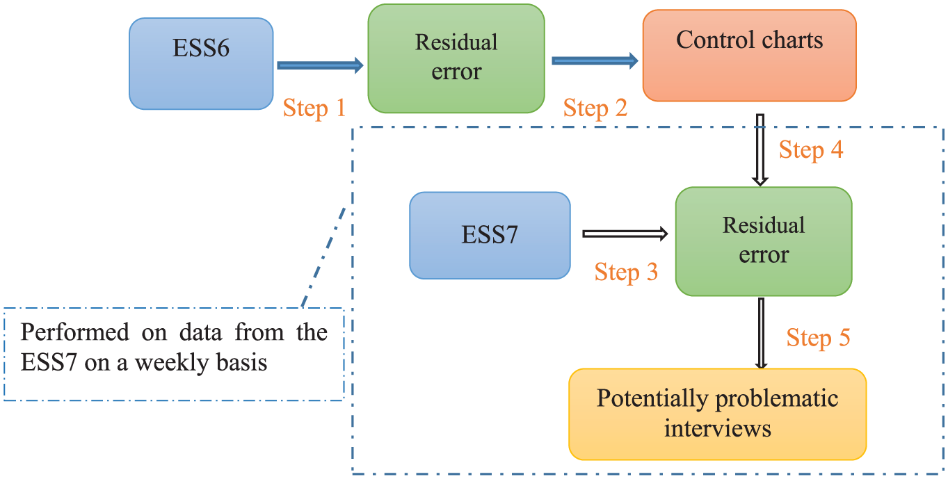
The application of control charts to the ESS7 proceeds in several steps and is shown in Figure 3 above. The steps are as follows:

Step 1: Control for the impact of the respondent factors (listed in Table 3) on the interview duration from the ESS6.

Step 2: Build control charts on the residuals calculated from the regression model for the ESS6 (obtained in Step 1) and bring the process in control iteratively by excluding one interview at a time. The in-control process based on the ESS6 provides the process average and control limits used to monitor data from the ESS7.

Step 3: Control for the impact of the respondent factors (listed in Table 3) on the interview duration from the ESS7.

Step 4: Monitor the residuals obtained from Step 3 for the ESS7, using the process average and control limits estimated in Step 2.

Step 5: Identify potentially problematic interviews for the ESS7 by modeling the residuals using control charts and find the related interviewers.

The analyses in Step 1 and Step 2 are accordingly based on all the ESS6 data before going on to assess the ESS7 data. By contrast, the analyses of the ESS7 (Step 3, Step 4, and Step 5) are based on the cumulative interviews available in each fieldwork week. Specifically, when interviews from Week 1 are available, a regression model is built and the residual errors from the model are examined using a control chart. Each of these interviews is assigned a status (normal or problematic). In Week 2, the model is rebuilt based on the interviews completed in both Week 1 and Week 2, and the residual errors, composing two subgroups–Week 1 and Week 2–are examined via control charts. In each of the subsequent weeks, the model is updated to take the new data into account. A new series of residual errors, as well as their corresponding status, is then obtained every week. An interview identified as problematic in Week 1 is not necessarily problematic in later weeks, as its residual error, and the average and standard deviation of Week 1 all change with the regression model estimated in each particular week. In this way, this procedure rechecks the decisions on old interviews whenever new data are available.

Figure 3.

The process for applying control charts to interview duration data from the ESS7.

To address RQ1, we develop the above procedure for monitoring interview duration while controlling for the impact of respondent characteristics, with the aim of enabling the identification of problematic interviews in the ESS7 from the first week of fieldwork onward. By tracking the status of each interview to examine the consistency of our findings over time, we can answer RQ2: whether we can apply SPC control charts to interview duration during survey data collection.

Results

Phase I, Monitoring of the ESS6

In the ESS6 in Belgium, four out of the total 1,869 interviews contain missing values on the list of variables shown in Table 3, and were therefore removed. To execute the first step of our procedure, we specify the regression model for data from the ESS6. With nonsignificant variables removed (eduyrs), the multiple regression model for all available interviews from the ESS6 (1,865 in total) is specified as follows:

\begin{array}{l} \log (y_{i}) = 5.1492 + 0.0026 a g e_{i} + 0.0560 r e s c l q_{i} \\ - 0.0455 i n t l n g a_{i} - 0.0053 n o t a p p_{i} \\ - 0.0196 n_{i} + e_{i} \end{array}

Older respondents take more time to answer questions, the interview duration increases when respondents frequently ask for clarification, having fewer applicable questions reduce the interview duration, and the order in which interviews are taken has a negative effect on the duration. The interview language also significantly influences the duration: interviews taken in French are longer than those taken in Dutch. This confirms our expectations and makes it clear that these variables are relevant to control for.

Using the R package qcc (Scrucca, 2004), the control charts based on the residuals ei $e_{i}$ are shown in Figure 4. The time points on the x-axis are the fieldwork weeks for the ESS6, with each point representing a subgroup of interviews completed in one particular week. The fluctuations of the control limits are due to the fact that the number of completed interviews is different for each week. The weekly average for ei falls between the control limits, while the weekly standard deviation of ei falls outside the control limits in Week 2 (represented by a red square).

Figure 4.

Control charts for the ESS6 ei where the process is not in control.

As already detailed, analysis of the ESS6 offers the necessary information to monitor the ESS7 by providing the process average and control limits. To achieve this, any interviews responsible for an outlying week should be excluded to bring the process back in control. As the average of Week 2 is around the CL and the standard deviation is above the UCL, according to Table 2 we take the boxplot of $e_{i}$ ei from the multiple regression (see Figure A1 in the appendix) into consider ation to help determine the responsible interview. As a result, the interview with the largest ei in Week 2 is considered as most responsible. This interview is also the longest interview completed in the ESS6 (lasting for 142 min). The control charts are recalculated with this interview dropped and the process is then considered as being in control, as no weeks fall outside the control limits (see Figure A2 in the appendix).

The estimated parameters on the $\bar{x}$ chart ( $\bar{x} = 0$ , $s_{x} = 0.2245$ ) and s chart ( $\bar{s} = 0.2236$ , $s_{s} = 0.2264$ ) will be used to monitor the ESS7. Apart from the interview identified, the other interviews from the ESS6, which we define as “normal,” range from 11 min to 81 min.

Phase II, Monitoring of the ESS7

The data collection period for the ESS7 in Belgium lasted for 20 weeks, which differs from the ESS6. However, only a small number of interviews were completed in the last few weeks (e.g., eight interviews in the penultimate week). A problem is that standard deviation is not a proper estimate of the variation in small subgroups. Therefore, we limit ourselves to monitoring the 1,642 interviews completed in the first 14 weeks, which accounts for 93% of the total. The subgroup size ranges from 63 to 170 interviews.

Using the Phase I control charts built on the in-control data from the ESS6, interviews completed in the ESS7 can be examined from the start of the fieldwork. First, multiple regressions are applied on the cumulative interviews available in each week. To avoid estimation problems, it is necessary to exclude the extreme values of durations when modeling. To guide the exclusion, the in-control data from a previous round can be considered relevant and informative. As detailed, after removing one exceptionally long interview, we obtain a subset of in-control interviews for the ESS6, which range from 11 min to 81 min. This range is relatively large compared with the one percentile and 99 percentile for all the ESS6 interviews (respectively 19 min and 65 min). Therefore, interviews from the ESS7 that are shorter than 11 min or longer than 81 min are temporarily ignored for modeling. These interviews (shorter than 11 min or longer than 81 min) are not excluded from the monitoring, however, as the effects of respondent characteristics have not yet been considered. In short, only interviews within the range of 11 min to 81 min are used to estimate the parameters of the multiple regression, but the estimated model is applied to all the interviews with a view to obtaining the residual errors.

As shown in Table 4, more interviews are completed as the data collection progresses, making more interviews available (S) and usable for modeling (s). The effect of age (age) and the frequency of respondents asking for clarification (resclq) are found to be significant and positive from the start of the ESS7. By contrast, education level (eduyrs) has no significant effect throughout the fieldwork. The other variables—including interview language (intlnga), the number of not applicable questions (notapp), and interview order (n)—enter into the model in Week 3. Moreover, the model estimated in Week 2 has found the “correct” signs of the parameters. With regard to the size of the estimated parameters, we can see that the adjustments in the estimated coefficients of age, frequency of asking for clarification, and the number of not applicable items are small over time, whereas the variability in the estimated coefficients of the interview order and interview language are relatively larger.

Table 4.

Results of Multiple Regressions for the ESS7.

Week	Data source	S	s	intercept	age	eduyrs	resclq	intlnga	notapp	n
1	Week1	75	75	4.275*	0.004*	−0.002	0.094*	0.0330	−0.004	0.010
2	Week1-2	230	226	4.679*	0.003*	−0.004	0.072*	−0.082*	−0.005*	−0.012
3	Week1-3	400	394	4.649*	0.004*	−0.005	0.067*	−0.080*	−0.005*	−0.019*
4	Week1-4	568	561	4.421*	0.003*	−0.003	0.073*	−0.072*	−0.004*	−0.024*
5	Week1-5	707	698	4.549*	0.003*	−0.003	0.067*	−0.063*	−0.004*	−0.023*
6	Week1-6	865	850	4.591*	0.003*	−0.004	0.063*	−0.061*	−0.004*	−0.018*
7	Week1-7	956	938	4.619*	0.003*	−0.003	0.061*	−0.060*	−0.005*	−0.017*
8	Week1-8	1,028	1,007	4.687*	0.003*	−0.003	0.061*	−0.058*	−0.005*	−0.018*
9	Week1-9	1,099	1,076	4.734*	0.003*	−0.002	0.062*	−0.068*	−0.005*	−0.019*
10	Week1-10	1,249	1,223	4.654*	0.003*	−0.002	0.065*	−0.069*	−0.005*	−0.016*
11	Week1-11	1,363	1,336	4.695*	0.003*	−0.002	0.065*	−0.067*	−0.005*	−0.013*
12	Week1-12	1,463	1,434	4.671*	0.003*	−0.003	0.067*	−0.062*	−0.005*	−0.011*
13	Week1-13	1,579	1,545	4.612*	0.003*	−0.001	0.061*	−0.065*	−0.005*	−0.011*
14	Week1-14	1,642	1,606	4.619*	0.003*	−0.002	0.059*	−0.064*	−0.005*	−0.009*

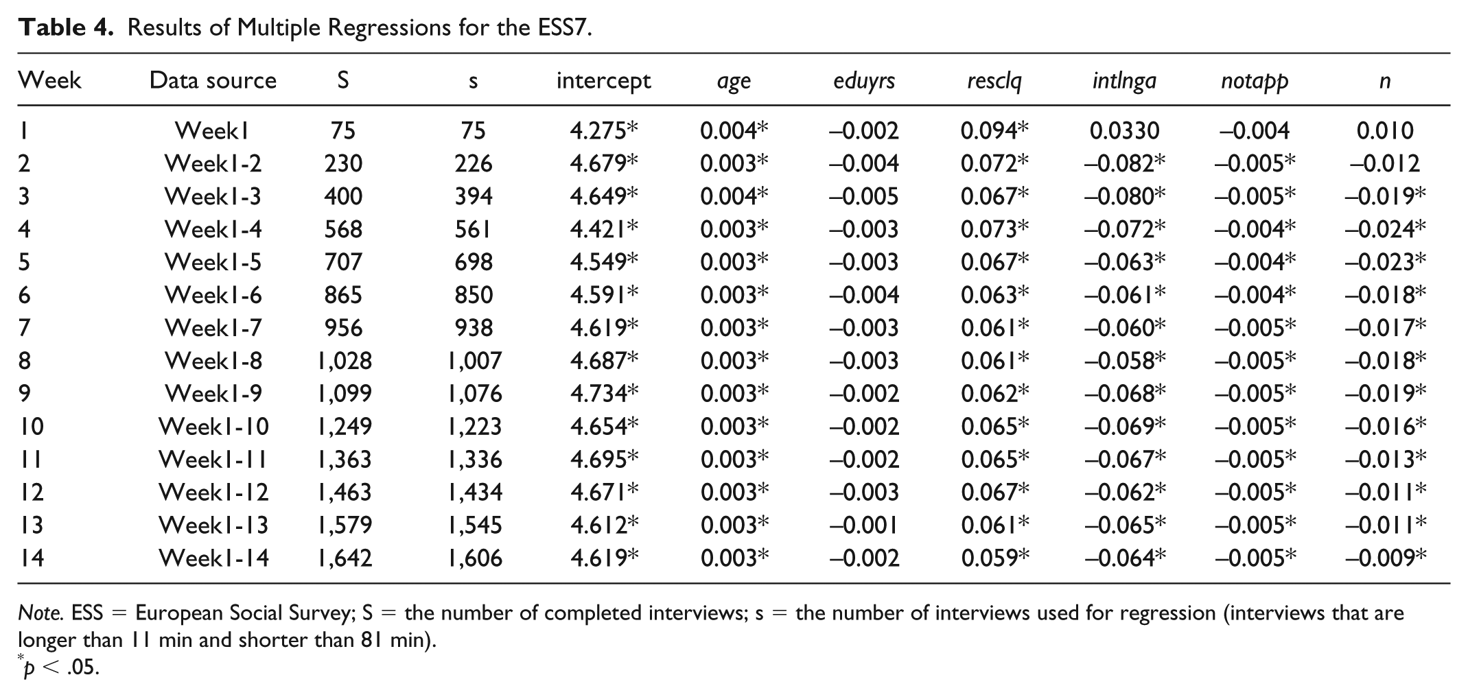
Note. ESS = European Social Survey; S = the number of completed interviews; s = the number of interviews used for regression (interviews that are longer than 11 min and shorter than 81 min).

p < .05.

In sum, the results suggest that the regression model built in an early phase of the fieldwork (Week 3) has already captured the main characteristics (significance, sign, and size) of the effects of these variables on interview duration.

Next, the residual errors from each of the 14 regressions are calculated and examined. The control limits are calculated based on the known parameters ( $\bar{\bar{x}}, s_{x}, \bar{s}, s_{s}$ ), estimated in Phase I, and the variable subgroup sizes in Phase II. In total, 14 control charts are obtained using R package qcc (Scrucca, 2004). The first examines whether the 75 residual errors from the first regression (corresponding with the 75 interviews completed in Week 1) are in control. The second control chart examines whether the 230 residual errors from the second regression (corresponding with the 75 interviews completed in Week 1 and 155 interviews completed in Week 2) are in control. Taking the second control chart for instance (Figure 5), Week 1 is in control, whereas Week 2 is not in control, with an extremely large standard deviation. Looking at Week 2 in greater detail, one interview recorded as 615 min is identified as being responsible for the too large standard deviation, and is therefore assigned a temporary status of problematic. The other control charts are not presented to be concise.

Figure 5.

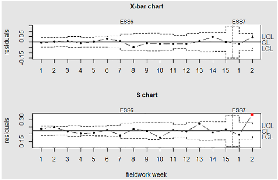
Control charts examining Week 1 of the ESS7.

Moving on from the first control chart (examining interviews completed in Week 1), one by one, to the 14th control chart (examining all interviews from these 14 weeks), we simulate the actual conditions in an ongoing survey data collection. As the survey progresses, more information is available for the process, and the status of interviews (not available yet, normal, or problematic) is updated. For example, an interview that was completed in Week 1 has its status updated in each of the following weeks.

Figure 6 presents how the status of each interview changes over time. The x-axis shows the weeks of fieldwork in which an interview’s status is determined (based on the data available up to that week) and assigned. This means that the points on x-axis correspond to the models listed in Table 4. The y-axis indicates the interview ID number. Interviews completed in the same fieldwork week are displayed in one subplot. From the upper left-hand corner to the lower right-hand corner of the picture, the subplots are arranged by week number from Week 1 to Week 14. Colors are used to indicate the status of the interview: not available yet (white), normal (gray), or problematic (red). The Week 1 model in Table 4, for example, is (only) related to the first point on x-axis in all subplots. The interviews completed in later weeks, displayed in the second to the last subplots, hence all have status of “not available” at the first point on x-axis. Of course, the later an interview is completed, the more weeks for which its status is not available and the fewer weeks left to update the status. Specifically, the interviews completed in Week 1 are examined 14 times from Week 1 until Week 14, but the interviews completed in Week 14 are only examined once, in Week 14.

Figure 6.

The status of interviews over fieldwork weeks.

First, we look at the whole process by examining how the status of each interview changes over fieldwork weeks. Interviews completed in Week 1 and Week 5 are determined consistently as in control (normal) until the end of the fieldwork. For interviews completed in Week 2, one interview is considered as problematic consistently in the following 12 weeks, whereas another problematic interview is not identified until the last week. For Week 6, one interview is only flagged up in 2 weeks but no longer later on, and another interview is rejudged as normal in the last four weeks. Similarly, two interviews from Week 8 are associated with inconsistent decisions in the following weeks (one changes from normal to problematic, and the other one the opposite). Decisions on interviews completed in the other weeks are constant over time. In sum, decisions on five interviews, which accounts for 0.3% (5/1,642) of the total interviews we monitor, are subject to change as the survey progresses. Thus, for the vast majority of interviews, our determination about whether they are normal or problematic remain consistent over the fieldwork.

Second, we focus on the results obtained in Week 14 when all the interviews have been assigned their final status. Some 27 interviews out of a total of 1,642 are identified as problematic, and 19 out of 150 interviewers are associated with these interviews. For these 27 interviews, we examined their interview order in the associated interviewer’s workload and the respondent profile, but no systematic conclusion (such as the first interviews are more likely to be outliers) can be reached to explain the causes. Of these 27 interviews, 25 had been immediately identified after completion. It should be remembered that in “Data” section, we found extreme values in the distribution of log-transformed interview duration data from the ESS7 (consisting of 1,759 interviews). For the 1,642 interviews we monitored in this study, we found that 25 fell 3 times the interquartile range (IQR) below the first quartile or above the third quartile. Out of these 25 interviews, 23 were identified by our procedure. This means around 92% (23/25) of extreme observations (defined by $3 \times IQR$ ) identified after survey data collection can be identified by our procedure during survey data collection.

In conclusion, with regard to RQ1 (how to monitor interview duration during survey data collection), we developed a dynamic procedure (Figure 3) that facilitated both the monitoring of the ESS7 from the first fieldwork week and the rechecking of the previous results whenever more information was available, while controlling for the impact of respondent characteristics. Addressing RQ2 (do we have consistent results over time?), by using the developed procedure, the results suggest that our decisions about whether an interview is normal or problematic at an early phase of the fieldwork are almost the same as those when more information is available at a later phase.

Conclusion and Discussion

This study was motivated by the fact that despite general agreement about the usefulness of SPC tools in monitoring paradata, examples of applying SPC from an early phase of survey fieldwork are rather rare. This study’s aim was twofold: (a) to explore a procedure for monitoring paradata to allow survey practitioners to identify interviews and interviewers for which closer scrutiny is needed right after the survey data collection starts and (b) to evaluate whether the identifications based on our procedure are reliable over time.

Taking one type of paradata—interview duration—as an example, this study has established a procedure for monitoring the ESS7 in Belgium from its start by using data from the ESS6 as Phase I. To enhance the comparability of data from different rounds of the ESS, only the core modules were included when measuring the duration of interviews. Moreover, we used multiple regression to single out the effects of respondent characteristics on interview duration. SPC control charts were applied to the residual errors from the multiple regression to detect any exceptionally long and short interviews. Although first suggested in Couper and Kreuter’s (2013) study on response times, this SPC-oriented use of residuals has not previously been practically applied or tested. Furthermore, our procedure is dynamic. We simulated the real data collection process in the ESS7 by using cumulative data available for each fieldwork week. As the survey progressed, more and more information became available with which to decide whether an interview was normal or problematic. The decisions made about the interviews were therefore recorded and updated along the survey process.

We found that when more data were available, only 0.3% of the total interviews were subject to changed decisions. In this regard, the results were reliable even for the first weeks, when information was limited. Out of the 27 interviews identified as problematic when all the information was available, 25 were immediately identified, which implies that the results were also efficient. What can be found afterward can already be found during the earlier stages of the survey data collection. Despite the relatively small percentage of the identified problematic interviews (1.64%, 27/1,642), we consider the use of control charts, as a tool for SPC, still relevant and in fact always necessary. The reason is that control charts are used not only to show when the process is out of control but also to show when the process is in control and only normal variations are taking place. Therefore, besides identifying a large number of problematic cases, SPC can also be used to assure that the quality of a process is good. With regard to the 27 identified interviews, an attempt was made to find the causes by examining the interview order and respondent profile, but no systematic conclusion was reached. However, we are confident that our work serves as a base for future studies on using more complex tools, such as machine learning techniques, to identify the causes of the outlying interviews.

Overall, the results of this study imply that survey practitioners can focus on the interviews for which further examinations are needed immediately, rather than waiting until the data collection has been completed. They could, for example, go back to the specific interviewer to investigate the situation, make use of more expensive evaluation tools (such as analyzing keystrokes, audio records, audit trail data, conducting re-interviews.), and reinstruct interviewers if applicable. There may be concerns about the timeliness of the interventions in practice. For example, for a specific interviewer, the retraining may only take place when he or she has already conducted a number of more interviews. However, the effects of the retraining is not confined to the present survey project but extends to the future, because interviewers—each a member of the interviewer staff—will probably not only work for one particular survey project but also other projects.

Moreover, the analysis in this study could help the practitioners concerned to give interviewers interactive feedback to guide their fieldwork. With estimated interview duration based on a respondent’s characteristics, an interviewer could be alerted during the interview when delivering survey questions too quickly or too slowly. In this regard, the use of control charts is in line with the ideas of responsive designs (Groves & Heeringa, 2006) and adaptive designs (Wagner, 2008) for monitoring key variables and guiding fieldwork interventions. The key variables are not limited to paradata like interview duration but more broadly any variables that are informative about survey data quality (e.g., indicators measuring certain response styles such as straightlining). Furthermore, as control charts provide a visual graphic presentation of the changes in a process over time, survey dashboards—which have been developed for a number of surveys (e.g., see Craig & Hogue, 2012; Lepkowski et al., 2010)—will be more informative and effective with control charts being integrated. However, as pointed out by Kreuter and colleagues (2010), this relies crucially upon the timely availability of the key data that control charts aim to monitor.

Unfortunately, the complexity of the survey conditions where interviews are conducted limits the adaptation of SPC tools to the survey context. First, the grouping of interviews by weeks limits the use of S charts. In survey settings, a relevant time scale (such as fieldwork days and weeks) is recommended to group the interviews (Jans et al., 2013). A related problem is that interviews can be distributed rather unevenly over time. In our study, for the last few weeks when the number of completed interviews is very small, an S chart is not an appropriate tool to monitor the variability of the data. The final few interviews completed in the last few weeks, however, are certainly among the most important to be monitored and evaluated. Future studies would benefit from investigating other possible ways of grouping interviews (e.g., groups of interviewers).

Second, applying control charts to residuals from regression models enabled us to single out the impact of respondent variables on interview duration, but also meant that a part of the information was not taken into account. For instance, information about the expected mean value of the interview duration when all variables are zero is contained in the intercept of the regression model. The residuals, on the other hand, always have a mean of zero on the X-bar chart. Further investigation could reveal the influence of the use of regression models on the outliers identified by control charts.

Third, the implementation of the control charts in this study is based upon the assumption that interviews completed in one fieldwork week, together with the corresponding contact forms, were available to fieldwork institution before the end of the week. Such an assumption, however, currently is still not easily satisfied in many face-to-face surveys. The reason is that, frequently, it is the interviewers themselves who decide when to submit the data to the fieldwork institution. Therefore, from a practical point of view, care must be taken to ensure that the delay between the collection of data by interviewers and the availability of the data for use is small enough for making meaningful interventions at the most appropriate time. However, we believe that with the rapid development of data collection technology, a wide variety of (para)data will be instantaneously available in more and more face-to-face interviews.

The limitations in the subgrouping of interviews, the combined use of regression models and control charts, and the practical requirements for the timely available data during fieldwork notwithstanding, this article marks a step forward to using paradata during survey data collection rather than retrospectively. Identifying problematic interviews and associated interviewers by monitoring interview durations could facilitate and intensify interventions during the survey data collection period, thus improving survey quality in a dynamic way.

Footnotes

Appendix

In Phase I, suppose we have k subgroups with the ith subgroup size being n i . For the ith sample, let x ¯ i be the subgroup mean, and s i be the subgroup standard deviation. Then

x ¯ ¯ = ∑ n i x i ¯ ∑ n i

and

S ¯ = ∑ n i s i ∑ n i

are the center lines on the X-bar and S control charts, respectively. The other parameters are listed on the left-hand side of Table A1 below. After all the outliers are removed iteratively in Phase I, the parameters in the Phase II control charts can be calculated based on the formulas listed on the right-hand side of Table A1. with n j representing the size of the jth subgroup of the new data.

Declaration of Conflicting Interests

The author(s) declared no potential conflicts of interest with respect to the research, authorship, and/or publication of this article.

Funding

The author(s) disclosed receipt of the following financial support for the research, authorship, and/or publication of this article: This study was financilly supported by China Scholarship Council (CSC No. 201509210005).

Notes

ORCID iD

Jiayun Jin

Author Biographies

Jiayun Jin is a PhD candidate at the Center for Sociological Research of the Catholic University of Leuven (KU Leuven). She is interested in the use of survey data and paradata to evaluate survey data quality from a measurement error perspective.

Caroline Vandenplas is a research assistant and has completed her PhD at the Center for Sociological Research of the Catholic University of Leuven (KU Leuven). Her doctoral dissertation examines “The Impact of Time and Timing on the Survey Process and Data Quality”.

Geert Loosveldt is professor at the Center for Sociological Research of the Catholic University of Leuven (KU Leuven) where he teaches Social Statistics and Survey Research Methodology. His research focuses on evaluation of survey data quality with special interest in the evaluation of interviewer effects and the causes and impact of non-response error.

References

Beullens

Loosveldt

Denies

Vandenplas

(2016). Quality matrix for the European social survey, round 7. Retrieved from https://www.europeansocialsurvey.org/docs/round7/methods/ESS7_quality_matrix.pdf

Brick

Tourangeau

(2017). Responsive survey designs for reducing nonresponse bias. Journal of Official Statistics, 33, 735-752.

Chakraborti

Human

S. W.

Graham

M. A.

(2008). Phase I Statistical Process Control charts: An overview and some results. Quality Engineering, 21, 52-62.

Chun

A. Y.

Heeringa

S. G.

Schouten

(2018). Responsive and adaptive design for survey optimization. Journal of Official Statistics, 34, 581-597.

Couper

M. P.

Kreuter

(2013). Using paradata to explore item level response times in surveys. Journal of the Royal Statistical Society: Series A (Statistics in Society), 176, 271-286.

Craig

T. L.

Hogue

(2012, March). The implementation of dashboards in governments division surveys. Paper presented at the Federal Committee on Statistical Methodology conference, Washington, DC.

Draisma

Dijkstra

(2004). Response latency and (para) linguistic expressions as indicators of response error. In S. Presser, M. P. Couper, J. T. Lessler, E. Martin, J. M. Rothgeb, & E. Singer (Eds.), Methods for testing and evaluating survey questionnaires (pp. 131-147). Hoboken, NJ: John Wiley.

Ferrer

(2007). Multivariate statistical process control based on principal component analysis (MSPC-PCA): Some reflections and a case study in an autobody assembly process. Quality Engineering, 19, 311-325.

Groves

R. M.

Heeringa

S. G.

(2006). Responsive design for household surveys: Tools for actively controlling survey errors and costs. Journal of the Royal Statistical Society: Series A (Statistics in Society), 169, 439-457.

10.

Heerwegh

(2003). Explaining response latencies and changing answers using client-side paradata from a Web survey. Social Science Computer Review, 21, 360-373.

11.

Jans

Sirkis

Morgan

(2013). Managing data quality indicators with paradata based statistical quality control tools: The keys to survey performance. In Kreuter

(Ed.), Improving surveys with paradata (pp. 191-230). Hoboken, NJ: John Wiley.

12.

Japec

(2006). Quality issues in interview surveys–some contributions. Bulletin of Sociological Methodology, 90, 26-42.

13.

Kreuter

Couper

Lyberg

(2010, July 31-August 5). The use of paradata to monitor and manage survey data collection. Paper presented at the Joint Statistical Meetings of the American Statistical Association, Alexandria, VA. Retrieved from http://www.asasrms.org/Proceedings/y2010/Files/306107_55863.pdf

14.

Kreuter

Olson

(2013). Paradata for nonresponse error investigation. In Kreuter

(Ed.), Improving surveys with paradata (pp. 13-42). Hoboken, NJ: John Wiley.

15.

Krosnick

J. A.

(1991). Response strategies for coping with the cognitive demands of attitude measures in surveys. Applied Cognitive Psychology, 5, 213-236.

16.

Lepkowski

Axinn

Kirgis

West

B. T.

Kruger

S. N.

Mosher

Groves

(2010). Use of paradata in a responsive design framework to manage a field data collection (NSFG survey methodology, Working papers, Report 10-012). Retrieved from https://www.researchgate.net/profile/James_Lepkowski/publication/236625287_Use_of_Paradata_in_a_Responsive_Design_Framework_to_Manage_a_Field_Data_Collection/links/543509d40cf2bf1f1f27e8bb/Use-of-Paradata-in-a-Responsive-Design-Framework-to-Manage-a-Field-Data-Collection.pdf

17.

Loosveldt

Beullens

(2013). “How long will it take?” An analysis of interview length in the fifth round of the European Social Survey. Survey Research Methods, 7, 69-78.

18.

MacCarthy

B. L.

Wasusri

(2002). A review of non-standard applications of statistical process control (SPC) charts. International Journal of Quality & Reliability Management, 19, 295-320.

19.

Malhotra

(2008). Completion time and response order effects in web surveys. Public Opinion Quarterly, 72, 914-934.

20.

Montgomery

D. C.

(2009). Introduction to statistical quality control. New York, NY: John Wiley.

21.

Oakland

J. S.

(2007). Statistical process control. Oxford, UK: Elsevier.

22.

Olson

Parkhurst

(2013). Collecting paradata for measurement error evaluations. In Kreuter

(Ed.), Improving surveys with paradata (pp. 43-72). Hoboken, NJ: John Wiley.

23.

Olson

Peytchev

(2007). Effect of interviewer experience on interview pace and interviewer attitudes. Public Opinion Quarterly, 71, 273-286.

24.

Revilla

Ochoa

(2015). What are the links in a Web survey among response time, quality, and auto-evaluation of the efforts done? Social Science Computer Review, 33, 97-114.

25.

Schouten

Peytchev

Wagner

(2017). Adaptive survey design. New York, NY: Chapman & Hall.

26.

Scrucca

(2004, November). Qcc: An R package for quality control charting and statistical process control. R News, 4(1), 11-17.

27.

Sirkis

Jans

Dahlhamer

Gindi

R. M.

Duffey

(2011, July 30-August 4). Using statistical process control to understand variation in computer-assisted personal interviewing data. Paper presented at the Joint Statistical Meetings, Miami Beach, FL.

28.

Stoop

Devacht

Billiet

Loosveldt

Philippens

(2003, September). The development of a uniform contact description form in the ESS. Paper presented at the 14th International Workshop for Household Survey Nonresponse, Leuven, Belgium.

29.

Stoop

Matsuo

Koch

Billiet

(2010, July 31-August 5). Paradata in the European social survey: Studying nonresponse and adjusting for bias. Paper presented at the Joint Statistical Meeting of the American Statistical Association, Vancouver, British Columbia, Canada.

30.

Vandenplas

Loosveldt

Beullens

Denies

(2018). Are interviewer effects on interview speed related to interviewer effects on straight-lining tendency in the European Social Survey? An interviewer-related analysis. Journal of Survey Statistics and Methodology, 6, 516-538.

31.

Vining

(2009). Technical advice: Phase I and phase II control charts. Quality Engineering, 21, 478-479.

32.

Wagner

(2008). Adaptive survey design to reduce nonresponse bias (Doctoral thesis). University of Michigan, Ann Arbor.

33.

Woodall

W. H.

(2000). Controversies and contradictions in statistical process control. Journal of Quality Technology, 32, 341-350.

34.

Yan

Tourangeau

(2008). Fast times and easy questions: The effects of age, experience and question complexity on web survey response times. Applied Cognitive Psychology, 22, 51-68.

35.

Zhang

Conrad

(2014). Speeding in web surveys: The tendency to answer very fast and its association with straightlining. Survey Research Methods, 8, 127-135.

The Evaluation of Statistical Process Control Methods to Monitor Interview Duration During Survey Data Collection

Abstract

Keywords

Introduction

Data

Method

An Introduction of Control Charts and the Two Phases

Drilling Down From an Outlying Week to Individual Interviews

Using Multiple Regression to Control for Respondent Characteristics

A Procedure for Applying Control Charts to the ESS7 Data

Results

Phase I, Monitoring of the ESS6

Phase II, Monitoring of the ESS7

Conclusion and Discussion

Footnotes

Appendix

Declaration of Conflicting Interests

Funding

Notes

ORCID iD

Author Biographies

References