
Abstract
Although there is already considerable research on the connection between the availability of substance and the prevalence of its use, the relative effect that one factor has on the other is rather unclear. The present study aims to scrutinize the mutual relationship between subjectively perceived cannabis availability and the prevalence of cannabis use among 15- to 16-year-old students, applying an integrative multilevel analytic framework. The Czech 2011 European School Survey Project on Alcohol and Other Drugs (ESPAD) dataset (N = 8,069 respondents) entered multilevel regression analyses to examine the sociogeographical inequalities in both perceived availability and adolescent frequent cannabis use (individuals [Level 1] nested within schools [Level 2] and localities [Level 3]). At the same time, the mutual relationship of the two cannabis indicators was demonstrated. At the level of individuals (Level 1), the simultaneous equations modeling (SEM) approach was applied to estimate the relative effect of perceived cannabis availability on the frequency of cannabis use and compare it vice versa. Adolescents coming from highly urbanized areas perceived cannabis to be more readily available, and they had a higher prevalence of frequent cannabis use. The higher availability mediated the sociogeographic inequalities in cannabis use. The locality unemployment rate was unrelated to either of the two cannabis indicators. At the individual level of the adolescent respondent, the effect of perceived availability on cannabis use appears to be much stronger than that of the effect of cannabis use on perceived availability when reversed. Perceived availability was found to mediate sociogeographic inequalities in cannabis use among Czechs adolescents. If a higher availability increases opportunities for adolescent substance misuse, then alongside other preventive measures, a spatially integrated approach should be applied in the national drug policy.
Keywords
Introduction
Background
Cannabis is the most frequently used illegal substance in Europe, with higher prevalence rates among adolescents and young adults (Hibell & Andersson, 2008; Vicente, Olszewski, & Matias, 2008). As adolescence is a specific period of transition in the individual’s lifespan characterized by multiple physiological, psychological, and social stressors, young people are more prone to indulge in risk behaviors and thus represent more vulnerable groups in this respect than those older in age.
While gaining firsthand experience with psychoactive substances might be considered as a rather natural phenomenon associated with adolescence (de Looze, Janssen, Elgar, Craig, & Pickett, 2015; ter Bogt et al., 2014), early cannabis use on a frequent basis can have serious consequences for the future mental and physical health of a young individual (Hall, 2009; Volkow, Baler, Compton, & Weiss, 2014). The research on determinants of the early onset of substance misuse, including frequent use of cannabis, is therefore particularly important for the public health agenda.
Several health risks are associated with cannabis use during adolescence, including the possible development of schizophrenia, anxiety, depression, suicidal tendencies, or drug dependence (Andréasson, Allebeck, Engström, & Rydberg, 1987; Arseneault et al., 2002; Copeland, Rooke, & Swift, 2013). The long-term effects of frequent cannabis use starting in adolescence were also found to increase the risk of altered brain development, cognitive impairment, reduced educational outcome, lower income, and lower life satisfaction (Fergusson & Boden, 2008; Volkow et al., 2014). In addition, cannabis as a psychoactive substance may serve as a potential gateway into other forms of illicit drug use with even more harmful consequences on an individual’s health, (Fergusson, Boden, & Horwood, 2006; Kandel, 1975), particularly among individuals predisposed to substance misuse and addiction.
From a global perspective, the prevalence of illicit drugs seems to be higher in more developed countries (Degenhardt & Hall, 2012). In most of these countries, restrictions and measures targeted at decreasing the availability of psychoactive substances are considered to be particularly important in preventing substance use and its related problems among youths (Knibbe et al., 2005). As documented by international surveys (Currie et al., 2012; Hibell et al., 2012), however, Czech adolescents have the highest levels of both availability and prevalence of substance use compared to other European teenagers. This applies to illicit substances, especially cannabis, as well as licit substances in general (alcohol, tobacco). The high availability and prevalence of substance use is considered to be due to the specific sociocultural environment of the Czech society, which is characterized by a high level of tolerance toward alcohol, tobacco, and cannabis consumptions (Csémy, Sovinová, & Procházka, 2012). A deeper understanding of the factors associated with the higher availability of drugs and their effects on substance use with a specific emphasize on the Czech adolescent population is, therefore, an issue that we focus on in the present article.
Multilevel Factors of Adolescent Cannabis Use
Regarding early cannabis use, multiple risk factors have been documented in public health research (European Monitoring Center for Drugs and Drug Addiction [EMCDDA], 2008; Substance Abuse and Mental Health Services Administration [SAMHSA], 2014). These factors operate at multiple levels, ranging from the level of the individual (e.g., age, gender, personality traits), through factors of school (e.g., the type of school attended) and the influence of adolescent peers, to factors operating at higher levels of the community and society as a whole. Starting in adolescence, the factors operating at higher levels grow increasingly important, as individuals increase their independence on families, spending more time in new and broader social contexts (Tucker, Pollard, de la Haye, Kennedy, & Green, 2013).
In the epidemiology of substance use, gender is recognized as one of the key factors for inequalities in adolescent cannabis consumption operating at the individual level (EMCDDA, 2008). Alongside biological differences (Fattore & Fratta, 2010), the higher prevalence of substance use among boys is considered to reflect a rather externalizing coping strategies with the adolescent transitional period; this contrasts with girls, where instead internalizing strategies are expected (Hurrelmann & Richter, 2006; Raithel, 2004; In: Pitel, Madarasová Gecková, Reijneveld, & van Dijk, 2013). Gender-differentiated attitudes toward substance misuse play a significant role as well (Mason, Mennis, Linker, Bares, & Zaharakis, 2014; Musher-Eizenman, Holub, & Arnett, 2003; Rienzi et al., 1996), including issues of unwanted loss of self-control resulting from intoxication among girls (Dahl & Sandberg, 2015). At the same time, cannabis use seen as a rebellious act might be attributed to a masculine behavior (Dahl & Sandberg, 2015). As documented by qualitative research studies, the gendered differences are particularly pronounced within frequent and intensive use of cannabis, rather than within experimental and occasional use (Measham, 2002; Warner, Weber, & Albanes, 1999).
In addition to gender, age is a significant predictor of cannabis use operating at the individual level as well. As adolescents’ health-related behaviors, including substance use, significantly change during this developmental period, the specific importance of appropriately timing an intervention, with a specific focus on the age of adolescence, is emphasized within both public health and the drug policy agenda (Currie et al., 2012). For example, with respect to cannabis use, according to the results of the 2011 Czech European School Survey Project on Alcohol and Other Drugs (ESPAD) survey, 21% of all the surveyed adolescent respondents declared that their first cannabis use occurred by the age of 14 years, 38% by the age of 15 years, and 43% by the age of 16 years (thus, the lifetime prevalence of cannabis use among these students was 43% in 2011; see Chomynová, Csémy, Grolmusová, & Sadílek, 2014). Although these data apply only to first experiences with the substance, they point to the growing importance of contextually determined factors on adolescent behavior during this specific developmental period.
Within structurally determined factors, the research has mainly focused on the effects of the socioeconomic status (SES) of an adolescent’s family, providing that adolescents from lower SES are characterized by a higher prevalence of cannabis use. In the meta-analysis, Lemstra et al. (2008) reviewed articles defining the family SES on the basis of parental income, parental education, employment status, and occupational classification. However, among adolescent students, the type of school attended may also be used as a proxy of students’ own SES (Berten, Cardoen, Brondeel, & Vettenburg, 2012; Gecková, van Dijk, Groothoff, & Post, 2002). As documented by earlier studies, students’ own educational levels, defined by attended school type, had a much stronger effect on substance use than the parental SES, including effects on the adolescent use of tobacco (Richter & Leppin, 2007), alcohol, cannabis, and other illicit drugs (Berten et al., 2012; Kážmér & Orlíková, 2017; Vereecken, Maes, & De Bacquer, 2004).
There are two mechanisms going on behind the effect of school type on adolescent substance use. First, the selection of a school type influenced by parental SES, parental norms, and modes of behavior, as well as educational aspirations transmitted from parents to a young student, predicts the later SES and behaviors of an adolescent individual (Hagquist, 2000, 2007; Richter & Leppin, 2007). The second mechanism involves the effect of a specific school environment that may influence adolescent behavior through normative peer culture associated with substance use prevalent in schools with lower educational aspirations, less demanding school curricula, and lower educational motivations (Richter & Leppin, 2007). The two mechanisms are parallel and of a cumulative nature. The mechanisms indicate that students from disadvantaged backgrounds tend to cluster in lower SES school types, and being among substance-use favoring peers, they tend to adapt to the lifestyle of the social group prevalent in their educational track (Koivusilta, Rimpela, & Rimpela, 1999).
The specific focus of our study is the effects of risk factors operating at higher levels of both community and society, and we expand upon the theory behind them in greater detail in the next sections.
Theoretical Frameworks
In the criminology literature, several theoretical frameworks underlie the importance of availability as a risk factor conductive for a delinquent behavior. For example, the Routine Activity Theory (RAT) stipulates three conditions for such a behavior to occur: (a) a motivated individual, (b) an absence of capable guardianship, and (c) the opportunity for a behavior, all coming together in time and space (Cohen & Felson, 1979). The RAT was developed as a macro-level theory, explaining the prevalence of delinquency in relation to the structural changes of social organization during the specific social and economic development of society. These changes are characterized by new forms of (routine) activities of everyday life, associated with a lowered guardianship over individual, thus increasing opportunities for delinquency.
The RAT was later expanded by Osgood, Wilson, O’Malley, Bachman, and Johnston (1996) into Routine Activity Theory of General Deviance (RATGD), which linked the previous macro-concept of routine activities with a deviant behavior at the individual level. The authors proved the significance of the role of routine activities as a mediator between structural variables and individual deviance. According to the RATGD, unstructured activities with peers and the absence of effective control authorities provide individuals opportunities for a given behavior (Osgood et al., 1996). At the same time, the RATGD included a wider range of behaviors outside the scope of delinquency, including alcohol and cannabis use among youth.
In epidemiology of substance use, the concept of availability was discussed particularly within the Smart’s Availability-Proneness Theory (Smart, 1977), which stressed availability and access to substances as key factors in the development of substance misuse. The theory applies the proposition that drug use occurs when a prone individual is exposed to a high level of substance availability.
Complementing the abovementioned theories, which focus either on macro-societal contexts (Cohen & Felson, 1979) or on individual-level factors (Osgood et al., 1996; Smart, 1977), the Social Disorganization Theory (SDT) suggests that residential location and neighborhood socioeconomic characteristics may also play important roles for engagement in a risk and deviant behavior, independently from a person’s individual characteristics (Sampson & Groves, 1989). The theory builds upon sociological research of urban communities and emphasizes the structural dimensions of neighborhood disadvantage (e.g., spatial concentration of poverty, high unemployment rates, the presence of lower social class, social segregation, and residential instability), as well as social interactional processes, in conjunction with institutional mechanisms, which transmit neighborhood-level factors into individual behavior (Sampson, Morenoff, & Gannon-Rowley, 2002).
According to the SDT’s central concept of collective efficacy (Sampson, Raudenbusch, & Earls, 1997; Shaw & McKay, 1942), the protective effects of social ties and social cohesion are presumably more likely to manifest in a more rural and less urbanized neighborhood context. Contrasted to rural ones, in highly urbanized areas, rather higher anonymity and weaker informal social control is expected, including the possibly stronger influence of deviant and substance-using peer groups in the city (Donnermeyer, 1992; Wilson & Donnermeyer, 2006). Hence, more urbanized areas may provide adolescents with differentiated opportunities for a risk and/or deviant behavior, including a higher availability of illicit substances.
Spatially concentrated disadvantages and relative deprivation can also provide a differentiated context associated with higher rates of substance use. Deprivation may negatively affect social bonds between adolescents, their families, and schools. This can result in increased opportunities for bonding with deviant peers or other deviant individuals located close to adolescent (Oetting, Donnermeyer, & Deffenbacher, 1998). Congruently with the SDT, the possible lack of local institutional resources in deprived areas may result in both insufficient provision of prosocial activities for adolescents and a lack of control over individual and/or group behavior, thus increasing opportunities for deviance (Leventhal & Brooks-Gunn, 2000). In addition, the potential social exclusion present in highly deprived areas can result in an additional exposure to social stressors, which can lead to a higher prevalence of substance use in these areas as well. The possibly higher prevalence of substance use concentrated in disadvantaged areas (the so-called “disadvantage hypotheses”) was suggested by socioecological studies, including research on adolescent cannabis use (Hyman & Sinha, 2009; Karriker-Jaffe, 2011).
Previous Research on Availability and Adolescent Cannabis Use
Regarding the availability of psychoactive substances, several approaches have been used to measure this concept, each emphasizing different aspects. Some apply retail prices, drug seizures, perceived availability by users, or the general level of drug consumption as a reflection of availability per se (EMCDDA, 2008). However, these approaches have not yet gained special merit and are instead considered complementary. Einstein (1981) emphasized the multidimensionality of the concept and distinguished between physical, social, economic, legal, and conceptual availability. However, Smart (1977, 1980) only distinguished the actual availability (measured, for example, by financial costs, time needed to buy drugs, number of nearby sellers, and/or places to buy) and the perceived availability (as a subjective estimate). In the context of illicit drugs, he recommended the latter approach due to the lack of information at hand on the actual availability of substances.
Given the clandestine nature of illicit drug markets, surveys among the adolescent population often rely on indicators of perceived, rather than actual, substance availability (Bjarnason, Steriu, & Kokkevi, 2010). At the same time, in large-sample population surveys, the perceived availability is typically measured by a single item with responses on a simple Likert-type scale (Hibell et al., 2012). Although this might indicate a certain reductionism, this simple measure is considered to result from multiple variables (Smart, 1980; ter Bogt et al., 2014; ter Bogt, Schmid, Gabhainn, Fotiou, & Vollebergh, 2006), comprising both subjective and objective factors within the individual estimation of the phenomena (e.g., exposure to the substance, price, various modes of access to drugs such as market purchase and/or self-supply modes, social networks, psychological factors, or specific sociocultural context). Building on this previous research, the present paper’s approach is based on adolescent perceptions as well. In the following text, the term “availability” refers to the concept of perceived availability.
Several studies examined the effects of the perceived availability on adolescent cannabis use (e.g., Castro, Valencia, & Smart, 1979; Knibbe et al., 2005; Maddahian, Newcomb, & Bentler, 1986; Smart, Adlaf, & Walsh, 1994). These studies generally anticipate that high rates of availability can lead to a high prevalence of substance use as well. However, from a rather critical perspective, in the case of perceived availability measured at the individual level of respondent, it could also be expected that, in addition, substance use itself elevates the subjective estimation of availability, as regular substance users probably know where and how to obtain it. Furthermore, these particular studies are based on aggregate measures of both availability and substance use and do not distinguish between the effects operating at an individual level from those operating at higher, environmentally determined (sociogeographical) levels.
When reviewing the literature concerning the effects of perceived cannabis availability on substance misuse, it becomes apparent that only a few studies have taken these rather critical standpoints (Bjarnason et al., 2010; Piontek, Kraus, Bjarnason, Demetrovics, & Ramstedt, 2012; ter Bogt et al., 2006). By applying a multilevel analytical framework, the study by Bjarnason et al. (2010) examines the effects of the different rates of perceived availability on the prevalence of cannabis use among teenagers coming from 31 European countries. Adjusting for the individual covariates of respondents, the study underlines the importance of the societal level of substance availability on the frequency of cannabis use among the adolescent population. Although the authors overcome the methodological problems of potential fallacy inherent in previous ecological studies, the mutual relationship between the perceived availability of the substance and its use has not been examined any further. Furthermore, the study is rather extensive, and it does not elaborate on other specific factors (e.g., cultural, institutional, environmental) operating at lower, in-country levels. The authors, however, state the need for further research focusing on the specifics of each particular society.
Studies on sociogeographic inequalities in adolescent cannabis use are mostly cross-nationally oriented, drawing on international data from large prevalence surveys. Most of these studies are rather descriptive, applying a comparative framework for researching inequalities in prevalence rates among adolescents coming from various countries (e.g., Currie et al., 2012; Hibell et al., 2012; Hublet et al., 2015; Kokkevi, Gabhainn, Spyropoulou, & Risk Behaviour Focus Group of the HBSC, 2006; Kokkevi, Richardson, Florescu, Kuzman, & Stergar, 2007). However, an empirical examination of the factors driving the inequalities in prevalence rates has been the subject of only a few recent studies. In this respect, the cross-national studies conducted by ter Bogt et al. (2006), Piontek et al. (2012), and ter Bogt et al. (2014) underscore the significance of the structural factors operating at both individual and societal levels (factors of individual’s gender, family affluence vs. societal wealth, and the availability of cannabis measured at the aggregate country level).
Similar to the cross-national studies, little research has been devoted to studying the sociogeographic factors of adolescent cannabis use operating at the regional, in-country levels. Most of the recent research aimed to test the significance of the factors suggested either by the abovementioned SDT theory (Bernburg, Thorlindsson, & Sigfusdottir, 2009; de Looze et al., 2015) or by the disadvantage hypotheses (Fite, Wynn, Lochman, & Wells, 2009; Ford & Beveridge, 2006; Pedersen & Bakken, 2016; Snedker, Herting, & Walton, 2009; Tucker et al., 2013). However, relatively few of the studies applied the rigorous multilevel analytical framework, and moreover, the empirical results are inconsistent. Some of the studies prove the significance of the factors operating at the examined in-country levels (de Looze et al., 2015; Fite et al., 2009; Tucker et al., 2013), and some of the studies do not prove it (Ford & Beveridge, 2006; Pedersen & Bakken, 2016) or even provide counterfactual results pertaining to the suggested hypotheses (Snedker et al., 2009); for a recent review, see Karriker-Jaffe (2011). Furthermore, most of these studies were conducted in the United States and in Canada, with only a couple of studies focusing on adolescents in European countries (Bernburg et al., 2009; Pedersen & Bakken, 2016).
Studies on urban–rural inequalities in adolescent cannabis use are even rarer. Some studies were conducted in the United States (Cronk & Sarvela, 1997; Donnermeyer, 1992; Van Gundy, 2006), in the United Kingdom (Miller & Plant, 1999), and later in other European countries (Kážmér, Dzúrová, Csémy, & Spilková, 2014; Licanin et al., 2002; Pitel, Madarasová Gecková, van Dijk, & Reijneveld, 2011; Schmid, 2001; Spilková, Pikhart, & Dzúrová, 2015). The studies from the United States emphasized lowering urban–rural inequalities in adolescent cannabis use from the mid-1970s through the 1990s (Cronk & Sarvela, 1997; Donnermeyer, 1992), with possibly higher rates of illicit substance use among adolescents in rural areas in recent periods (Coomber et al., 2011; Lambert, Gale, & Hartley, 2008; Martino, Ellickson, & McCaffrey, 2008; Van Gundy, 2006). Contrary to the United States, studies from Central Europe (Czechia, Slovakia, Switzerland, and Bosnia and Herzegovina) have found a higher prevalence of cannabis use among adolescents in urban areas as compared to those from rural ones. Therefore, more empirical research on this topic is needed as well.
Aims of the Paper
Given both the abovementioned limitations of the previous research and inconsistencies in the empirical results, this article addresses the relationship between the perceived availability and frequency of cannabis use in the specific Czech multilevel perspective. The emphasis on adolescents coming from Czechia is reinforced by the specific position of the country, characterized by a high level of both availability and cannabis use among youths.
The analysis of this article is divided into three steps. In the first step, the relationship between availability and frequent cannabis use is examined at the Czech national level, applying the time series data available from cross-sectional surveys conducted since 1995. In the second step, sociogeographic inequalities in both cannabis indicators are examined with respect to the Czech in-country (regional) levels. In the final step, this article scrutinizes the mutual relationship between the perceived availability and frequency of cannabis use at the individual level of the adolescent respondent.
In the analyses of sociogeographic inequalities, integrative multilevel modeling is applied. The multilevel models are adjusted for a set of lower level sociodemographic confounders (the effects of age, gender, and type of school attended), which were identified in number of the previous Czech studies (see Chomynová et al., 2014; Csémy, Chomynová, & Sadílek, 2009; Csémy, Lejčková, Sadílek, & Sovinová, 2006). In the multilevel analysis, we use the terms “environmental” and “regional” to refer to sociogeographic inequalities operating at the level of Czech localities. The sociogeographic dimension is represented here by two particular measures: (a) degree of urbanization as measured by the population size of locality and (b) locality unemployment rate, as the measure of locality socioeconomic disadvantage.
The results of multilevel models serve as a conceptual base to analyze the mutual relationship between the cannabis indicators at the individual level, conducted in the final part of the paper. As ordinary regression analysis cannot deal with reciprocal relationships between two or more dependent variables, we apply an approach based on simultaneous equations modeling (SEM). This makes it possible to estimate such a nonrecursive system of equations, provided that the identification problem is solved (Acock, 2013; Felson & Bohrnstedt, 1979). The results of the prior regression analyses are, therefore, presented and discussed in conjunction with the final SEM model.
Data and Methods
Sample and Design
In this article, individual respondent data on cannabis use indicators of the Czech school-aged population were analyzed. The data were obtained under the European School Survey Project on Alcohol and Other Drugs (ESPAD). As a main data source, the Czech cross-sectional dataset surveyed in 2011 was used. As an additional data source, a series of Czech national ESPAD reports published from 1995 to 2011 were applied too. The additional source was used for an introductory analysis of temporal changes of cannabis indicators among adolescent Czechs as compared to other European teenagers (1995-2011).
In Czechia, the National Monitoring Center for Drugs and Addiction, in collaboration with Prague Psychiatric Center, conducted the survey. Data collection took place in 113 localities (mean number of respondents per locality M = 71.4, SD = 72.5) and 364 schools of four different types (Chomynová et al., 2014). The following four school types are included: elementary schools (9th grade, 28.0% of students), secondary grammar schools (21.2% of students), secondary schools with leaving exams (28.1% of students), and vocational training schools (22.7% of students). Schools were randomly sampled according to the type of school and 14 administrative regions from the school register held by the Ministry of Education of the Czech Republic. The purpose of surveying was to ensure that data would be both nationally and regionally representative and thus would enable obtaining reliable estimates of substance-use–related indicators of the Czech adolescent population.
In the analysis, a total sample of 8,069 Czech school-aged respondents (15.0-16.9 years) was used; only those with nonmissing data on both cannabis use and perceived cannabis availability were included. Regarding the introductory analysis of temporal changes of the cannabis indicators among Czech adolescents as compared to other European teenagers (1995-2011), we had to limit it to data provided by countries participating in each survey period of the ESPAD project (see note in Figure 1 for details).
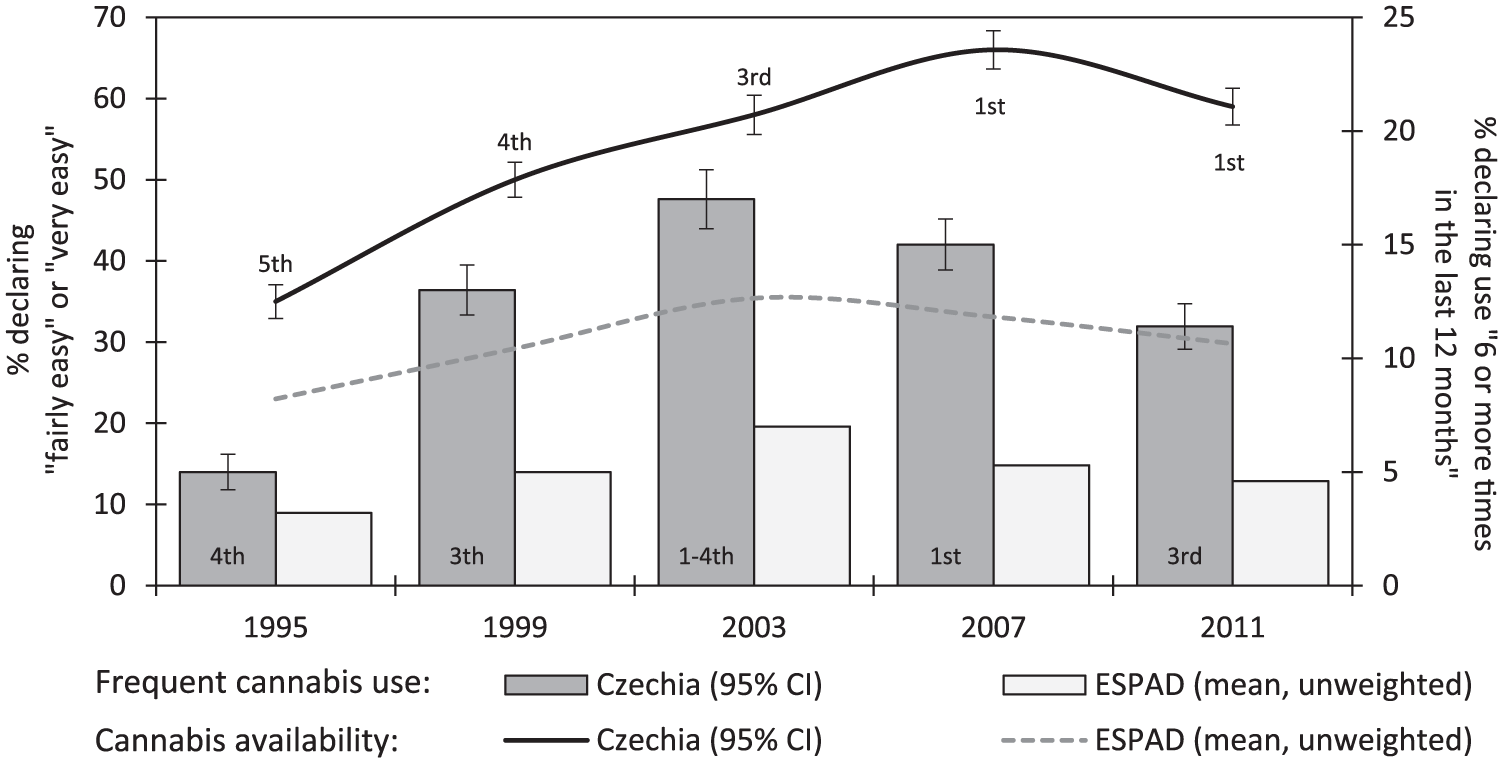
Perceived cannabis availability (left axis) and prevalence of frequent cannabis use (right axis) among European adolescents, Czechia compared to other ESPAD countries, time series from 1995 to 2011.
Ethical Considerations
The study was carried out as an anonymous questionnaire survey in school settings whereby student participation was voluntary. No ethical committee approval for the data collection was required; parental consent was not necessary as the age of the respondents was not below 15 years.
Dependent Variables
In the analysis, two dependent variables were used: (a) subjectively perceived cannabis availability and (b) cannabis use in the last 12 months. These two variables were considered as mutually interconnected, one variable affecting the other and vice versa.
Perceived cannabis availability was questioned as follows: “How difficult do you think it would be for you to get marijuana or hashish (cannabis) if you wanted?” Answers varied between 1 = “impossible”, 2 = “very difficult”, 3 = “fairly difficult”, 4 = “fairly easy”, 5 = “very easy”, and 6 = “don’t know”. Those reporting fairly easy or very easy were considered as cases reporting high levels of perceived availability. This coding was applied in Steps 1 and 2 of the statistical analysis. For construction of the simultaneous equations model in Step 3, an original ordinal scale between 1 and 5 was applied, ensuring that all of the information obtained in the data were used to estimate the parameters obtained by the simultaneous model. 1
Frequent cannabis use was based on the question on cannabis use in the last 12 months: “On how many occasions (if any) have you used marijuana or hashish (cannabis) during the last 12 months?” with answers varying between “0 occasions”, “1-2”, “3-5”, “6-9”, “10-19”, “20-39”, and “40 or more”. Students who reported cannabis use of 6 or more times during the last 12 months were coded as frequent cannabis users. 2 In Step 3 of the statistical analysis, the entire 7-point ordinal scale was applied to the simultaneous equations model, similarly to the previous case of perceived cannabis availability.
Independent Variables
In the regression analysis, respondent’s gender and age were used as conventional controlling variables. As the type of school attended by adolescent respondents was found to be strongly related to the prevalence of both licit and illicit substance use in all the previous Czech ESPAD surveys (Chomynová et al., 2014; Csémy et al., 2009; Csémy et al., 2006), the four different school types were included as controlling variables too.
To analyze sociogeographic inequalities in cannabis indicators, data on both population size of locality and locality unemployment rate were obtained from the 2011 Population and Housing Census of the Czech Republic and merged with the 2011 ESPAD dataset. In the analysis, the data were grand-mean centered. In the case of population size, the logarithmic transformation (common log) was applied, rather than the original values of the population size of locality.
Four independent variables (gender, age, type of school, and population size of locality—common log) were applied as instrumental variables in the SEM model, conducted in the last step of the analysis (Step 3). Two of them served for identification of perceived cannabis availability (population size of locality, age of respondent) and two for identification of cannabis use, respectively (gender and type of school attended). As the locality unemployment rate was found to be a nonsignificant predictor of neither of the two cannabis indicators, it was omitted from the SEM.
Statistical Analysis
The analysis included three steps based on the spatial level of data aggregation: national, regional, and individual. In Steps 1 and 2, correlation and regression analyses were conducted in Stata 15; in Step 3, SEM was applied via Stata’s 15 Structural Equation Modeling Module (StataCorp, 2017).
In Step 1, the introductory analysis of temporal changes of the two cannabis indicators from 1995 to 2011 was conducted, comparing Czech adolescents with other European countries. To show how the indicators relate to one another at the national level, the 1995-2011 time series of the Czech prevalence rates, and the Pearson correlation of the between-survey changes of the two cannabis indicators, was computed.
In Step 2, separate multilevel logistic regression models were constructed on the two binary indicators: high level of perceived cannabis availability (fairly easy or very easy = 1; otherwise = 0) and frequent cannabis use (6 or more times in the last 12 months = 1; otherwise = 0). There were three partial aims of the analysis in Step 2:
To identify sociogeographic inequalities in perceived cannabis availability and the prevalence of frequent cannabis use among Czech adolescents with respect to population size of the locality (Models A1, A2, A3, and B1).
To examine the effect of locality unemployment rate on both perceived cannabis availability and the prevalence of frequent cannabis use (Models A1 and B3).
To examine whether different levels of the perceived availability of the substance can explain the sociogeographic inequalities in frequent cannabis use (Model B2).
To control for intra-class correlation in response variables among students surveyed within the same school and/or locality, the three-level data structure was applied in regression analyses 3 : respondent (Level 1) nested within school (Level 2) and locality (Level 3). The analysis was conducted by the Stata’s melogit procedure.
At the individual level of the Czech adolescent respondent (Step 3), the relative effect of one dependent variable on another was examined (i.e., the effect of the perceived cannabis availability on the frequency of cannabis use as compared to the reverse direction). Here, the analysis was conducted via the nonrecursive system of SEM.
Identifying the nonrecursive SEM model was achieved through specifying five hypotheses and instrumental variables for the two dependent variables, as defined in the paragraph below. Four of the five hypotheses referred to results obtained in the previous regression analyses conducted in Step 2. To maintain the statistical efficiency in estimating the SEM regression coefficients, particularly those used to identify the two dependent variables via instrumental ones, a simple one-level SEM model was specified in Step 3, rather than a SEM with a complex multilevel structure. The validity of the one-level SEM builds upon the previous results obtained by multilevel regressions conducted in Step 2. 4 At the same time, as Pearson correlation coefficients between categorical variables can lead to biased parameter estimates in SEM models, polychoric (eventually polyserial) correlations between the input variables were calculated prior the SEM analysis, as suggested elsewhere (Browne, 1984; Kupek, 2006).
The following five hypotheses were simultaneously tested within the SEM model: Hypotheses 1 and 2 were considered as primary, while Hypotheses 3 through 5 were considered as secondary.
Primary hypotheses:
Although perceived cannabis availability and cannabis use are strongly interconnected, the effect of cannabis availability on its use should be more pronounced than the vice versa relation.
Living in localities with a larger population makes it easier to obtain the substance, which subsequently elevates the individual’s frequency of cannabis use.
Secondary hypotheses:
3. Secondary school students from more educationally demanding schools use cannabis less frequently than those studying in less demanding (i.e., more practice-oriented) schools, which implicitly elevates the individual’s perceived availability.
4. Boys, compared to girls, have a higher level of cannabis use, which implicitly elevates the perceived availability of the substance as well.
5. With an increase in age, the perceived cannabis availability increases too, which subsequently elevates the individual’s frequency of cannabis use.
Hypotheses 2 through 5 identified the SEM model. As regards Hypothesis 3, schools were sorted by type following the relative study demands imposed on students. Elementary schools, however, had to be excluded from the SEM analysis. 5 This resulted in a smaller sample size in Step 3 (N = 5,806).
The five SEM hypotheses were supplemented by additional assumptions regarding the covariance between the explanatory variables identified prior to the analysis: population size of locality (common log) with type of school, gender with type of school, age with gender. 6 As error terms are typically highly correlated in a nonrecursive SEM model, these were allowed to correlate freely as well (see e1 vs. e2 in Figure 3; for a methodological discussion, see, for example, Acock, 2013, pp. 72-73; Arbuckle, 2012, pp. 129-136). This correlation in error terms was set to account for any additional unobserved factors with an effect on both of the dependent variables not explicitly included in the analysis (i.e., other personal characteristics of the individual such as self-control over substance use, the specifics of his or her family background, and additional specific factors present in the given school and/or locality) 7 .
Apart from the correlation of error terms, the additional assumptions on covariance in explanatory variables are, however, descriptive in nature and do not affect the substantive results of the SEM analysis. These are only mentioned for the sake of completeness and to help the reader fully interpret the results of the covariance structure of the variables used in the SEM model.
Statistical Results and Their Interpretation
Czechia as a Leading Country From the European Perspective
In Figure 1, period-specific prevalence estimates, together with 95% confidence intervals of the two cannabis indicators from 1995 to 2011, are plotted. The specific position of Czech adolescents among other European youth is also depicted, by both the cross-national rank of the Czech respondents and the (unweighted) mean of prevalence estimates across all countries participating in the ESPAD project.
Although there are only a few period-specific measurements of the two cannabis indicators at the Czech national level, the parallel trends suggest a strong relationship between them. The high value of Pearson correlation of the between-survey changes of the indicators documents this suggestion as well: Corr[(% Highly available w – % Highly availablew-1), (% Frequent use w – % Frequent usew-1)] = 0.821; w = 2, 3, 4, and 5.
In the second step, a more detailed analysis of both perceived cannabis availability and frequent cannabis use was carried out at the Czech in-country level. Table 1 presents descriptive statistics of the 2011 Czech national dataset and additionally the initial cross-tabulation of both cannabis indicators with independent variables.
Descriptive Statistics of the Czech 2011 Sample and Cross-Tabulation of Dependent Variables With Independent Predictors.
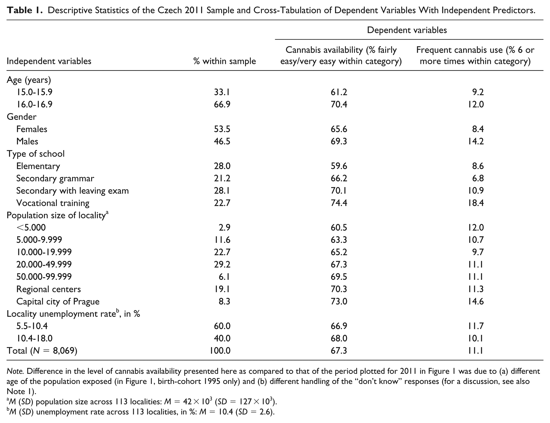
Note. Difference in the level of cannabis availability presented here as compared to that of the period plotted for 2011 in Figure 1 was due to (a) different age of the population exposed (in Figure 1, birth-cohort 1995 only) and (b) different handling of the “don’t know” responses (for a discussion, see also Note 1).
M (SD) population size across 113 localities: M = 42 × 103 (SD = 127 × 103).
M (SD) unemployment rate across 113 localities, in %: M = 10.4 (SD = 2.6).
Regarding the population size of locality, the level of cannabis availability continually increased from sparsely populated localities (60.5% within the category of <5.000 inhabitants) to the highest levels in the Capital City of Prague (73.0%; Table 1). The prevalence of frequent cannabis use was found to be higher only within the capital city (14.6%). The prevalence among adolescents from other localities with lower population size varied between 9.7% and 12%. With the locality unemployment rate, only minor differences in both cannabis indicators were observed. However, both cannabis indicators were significantly related to the sociodemographic variables (type of school, gender, and age), which could confound the initial results presented in Table 1.
A proper look at the significance of the sociogeographic factors is provided by the results from multilevel models, which are discussed in the following Tables 2 and 3. Altogether, six consecutive multilevel logistic regressions were conducted: three for the perceived cannabis availability (Models A1, A2, and A3) and three for frequent cannabis use (Models B1, B2, and B3).
Multilevel Binary Logistic Regression.

Note. Dependent variable—perceived cannabis availability (fairly easy or very easy = 1; otherwise = 0), Czechia, 2011. Ref.—reference group.
The increase in common logarithm (log 10) of the population size of locality by 1 corresponds to comparing two localities, whose population size ratio equals 10 (e.g., 1,000 vs. 100; 10,000 vs. 1,000, etc.)
Random intercept variance of the baseline model corresponding to Models A1 and A2 (three-level logit adjusted to age and gender only): Var[Level 2] = 0.083; Var[Level 3] = 0.024. Likelihood-ratio test versus one-level logistic model: χ2(df) = 39.9(2); p < .001.
Random intercept variance of the baseline model corresponding to Model A3 (three-level logit adjusted to age and gender only): Var[Level 2] = 0.064; Var[Level 3] = 0.019. Likelihood-ratio test versus one-level logistic model: χ2(df) = 22.9(2); p < .001. In Model A3, only respondents with no cannabis use in the last 12 months were included.
p < .05. **p < .01. ***p < .001.
Multilevel Binary Logistic Regression.

Note. Dependent variable—frequent cannabis use (Yes = 1; No = 0), Czechia, 2011. Ref.—reference group; Models B1 and B2 are two-level only.
Random intercept variance of the baseline model corresponding to Models B1 and B2 (two-level logit adjusted to age and gender only): Var[Level 2] = 0.464. Likelihood-ratio test versus simple logistic model: χ2(df) = 88.9(1); p < .001.
Random intercept variance of the baseline model corresponding to Model B3 (three-level logit adjusted to age and gender only): Var[Level 2] = 0.368; Var[Level 3] = 0.095. Likelihood-ratio test versus simple logistic model: χ2(df) = 95.1(2); p < .001.
p < .05. **p < .01. ***p < .001.
Table 2 summarizes the results of multilevel models conducted on perceived availability. The results indicate significant differences in availability at both the individual and regional (geographic) levels. Regarding the sociogeographic inequalities, the gradual increase in perceived availability with the population size of the locality (common log resp.; Model A1) was proved to be significant, even after adjustment for individual frequent cannabis use as a possible confounder (Model A2 and Model A3). 8 Contrasted with the population size, locality unemployment rate was not significantly related to the perceived availability of cannabis (Model A1). According to the type of school attended, students from vocational training schools reported the highest level of perceived availability, which gradually decreased with study demands imposed on students attending other types of school, while among students of elementary schools, the level of perceived availability was seen to be the lowest. At the same time, while there were only 2-year variations in the age of student respondents, the level of perceived availability significantly increased with age as well (Models A1 through A3).
The strongest association of cannabis availability, nevertheless, was found with the frequent cannabis use itself (Model A2). In this regard, we point to the fact that gender differences in perceived availability were not significant after adjusting for frequent cannabis use (compare Model A1 with Model A2, eventually with Model A3). Similarly, adjusting for frequent cannabis use (Models A2 and A3), no significant differences were found between students from secondary schools with leaving exams as compared to vocational training schools. It is therefore probable that differences in perceived availability between these groups of students resulted rather from the different rates of cannabis use as opposed to differences in availability as such. These preliminary results on the structure of the relationship between variables are examined by the SEM approach in the next section (Step 3 of data analysis).
The multilevel logistic regression approach was analogically applied for frequent cannabis use (Table 3). Yet, results of the analysis were slightly different than those described above in Table 2. Most of the sociogeographic inequalities in frequent cannabis use in Model B1 (Capital City of Prague vs. other localities) were explained after adjustment for perceived availability of the substance (Model B2). Nonetheless, the strong association between frequent use and perceived availability persisted (odds ratios [ORs] > 10 in Model B2, as well as in Model A2 in Table 2). As presented by Model B3, locality unemployment rate was unrelated to the prevalence of frequent cannabis use after adjusting for sociodemographic confounders.
The results in Table 3 also show that differences in frequent cannabis use between genders and different types of school remained significant in all three multilevel models. This is congruent with previous findings in Table 2 that different levels of perceived availability between boys and girls on one hand and different types of schools on the other hand were primarily related to different levels of cannabis use. Regarding the effect of age on adolescent frequent cannabis use, no significant effect was found among 15- to 16-year-old respondents, as opposed to the previous analysis in Table 2. Again, these preliminary results on the probable structure of relationships between variables are examined by the SEM approach in the next section.
Furthermore, Figure 2 summarizes sociogeographic inequalities for both perceived cannabis availability and frequent cannabis use with respect to the population size of localities, which was found to be significantly related to the analyzed cannabis indicators. The data represent marginal percentages (with 95% confidence intervals) as predicted by multilevel logistic models, adjusted for adolescent age, gender, and type of school attended. This comprehensive overview addresses the significance of the sociogeographical differentiation of the cannabis indicators, from sparsely populated localities to more densely populated areas. 9

Perceived cannabis availability (left axis) and frequent cannabis use (right axis) by population size of locality, marginal percentages, 95% CI, Czechia, 2011 (N = 8,069).
Perceived Cannabis Availability and Cannabis Use at the Individual Level
To estimate the mutual relative effect of perceived availability on the frequency of cannabis use at the individual level (Level 1), the SEM approach was applied in the third step. Table 4 presents polychoric (eventually polyserial) correlations between input variables as applied in the SEM analysis. Figure 3 presents the structure of the model itself. Unstandardized regression coefficients obtained by the SEM model, as well as identification diagnostics and model fit statistics, are available in Table 5; standardized regression weights are available in Figure 3. All regression weights are significant at p < .05 with a considerably good model fit, χ2(5) = 5.753, p = .331; root mean square average (RMSEA) = 0.005, and stable parameter estimation process (stability index of 0.427 well between −1 and +1). Identification diagnostics support conditions for both exogeneity (overidentification tests are not significant) and strength of instrumental variables (F-statistics of weak identification tests well above 10).
Polychoric/Polyserial Correlations Between SEM Input Variables, Czechia, 2011 (N = 5,806).

Note. Cannabis perceived availability and cannabis use—sorted ascending; age and population size of locality (log 10)—sorted ascending; gender (females = 0, males = 1); type of school—sorted ascending by relative study demands (i.e., vocational training schools—lowest, secondary grammar schools—highest). SEM = simultaneous equations modeling.
Polyserial correlations.
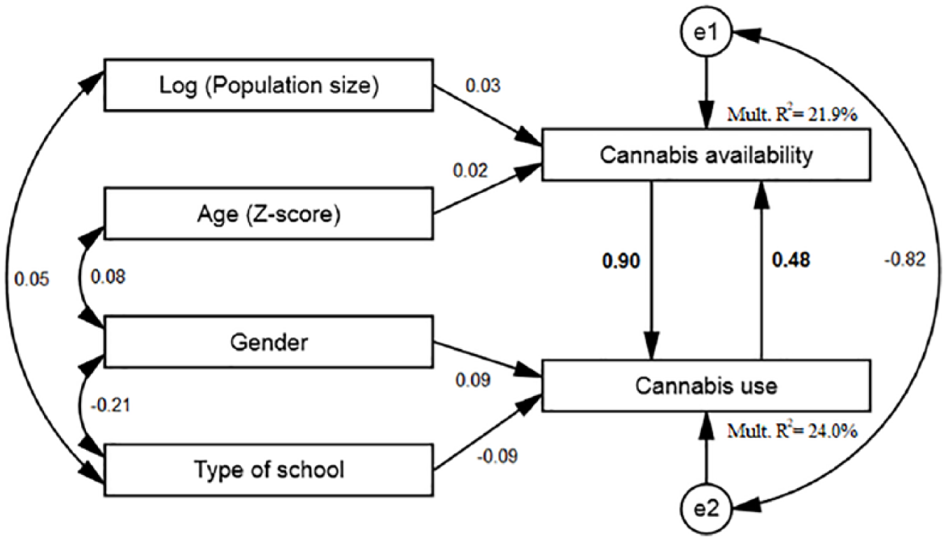
Standardized regression weights between perceived cannabis availability and cannabis use as outputs of the SEM analysis, Czechia, 2011 (N = 5,806).
Simultaneous equations modeling (SEM)—maximum likelihood estimates, Czechia, 2011 (N = 5,806).
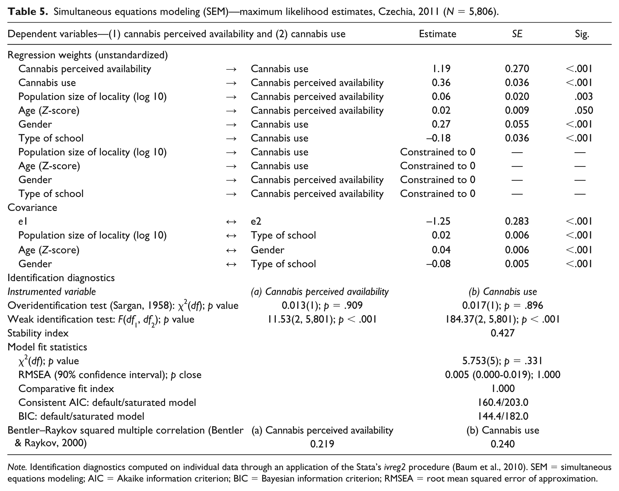
Note. Identification diagnostics computed on individual data through an application of the Stata’s ivreg2 procedure (Baum et al., 2010). SEM = simultaneous equations modeling; AIC = Akaike information criterion; BIC = Bayesian information criterion; RMSEA = root mean squared error of approximation.
According to the SEM model, there is significant mutual relationship between perceived cannabis availability and its use: higher perceived availability leads to higher levels of cannabis use, which in turn elevates the perceived availability. Nevertheless, the relative effect of cannabis availability on cannabis use, as estimated by standardized regression weights, is significantly higher than the effect of cannabis use on perceived availability when reversed, 0.90 > 0.48 in Figure 3; test of equality of standardized regression weights: χ2(df) = 4.20(1), two-tailed p value = .040.
The level of perceived cannabis availability is predicted by both the population size of the locality (common log) and the age of the respondent. Students in large Czech cities report higher levels of perceived availability of the substance. The higher the age of the adolescent, the higher the perceived availability as well. The SEM model also supports the hypotheses on cannabis availability as a mediator of the effect of both locality population size and age of respondent on the level of adolescent cannabis use (Table 5 and Figure 3).
The level of adolescent cannabis use is predicted by gender and type of school attended. In comparison to boys, girls have lower level of cannabis use. Adolescents from schools with higher relative study demands consume cannabis less often compared to those with lower study demands. The mediation of differences in cannabis availability among genders on one hand and among different types of school on the other hand by different levels of cannabis use is also supported by the SEM model (Table 5 and Figure 3).
Discussion
In general, our analyses have emphasized the importance of the specific focus on substance availability as a mediating factor between characteristics of the environment and the level of adolescent substance use. This was achieved by an analysis of the effect of a subjectively assessed level of cannabis availability on the frequency of cannabis use carried out with an integrative multilevel perspective.
Regarding the analysis carried out at the Czech national level, the changes in aggregate rates of both perceived cannabis availability and frequent cannabis use were strongly correlated (Pearson r = 0.821). Although the association between the indicators is rather well-documented in the research literature (e.g., Bjarnason et al., 2010; Freisthler, Gruenewald, Johnson, Treno, & Lascala, 2005; Hibell & Andersson, 2008; Johnston, O’Malley, Miech, Bachman, & Schulenberg, 2016; Piontek et al., 2012; Smart, 1977; ter Bogt et al., 2006), we conducted the analysis to examine the results from the national perspective with those obtained at lower levels of spatial aggregation and examined with a specific sociogeographic focus on the particular country, an aspect which is rather understudied.
In Czechia, issues of substance availability are especially important for the future health of the young generation. As presented in the introductory analysis (Figure 1), levels of both perceived cannabis availability and frequent cannabis use have been increasing continuously since the establishment of the Czech Republic in the early 1990s. Since the mid-2000s, Czech adolescents have even reported the highest levels of perceived availability in Europe and they also have one of the highest prevalence of frequent cannabis use.
Thus, Figure 1 suggests that the issues of cannabis availability and its use among adolescents is particularly relevant to the national drug policy. This can be attributed to the specific sociocultural environment of the Czech Republic, which is characterized by a high level of tolerance toward substance use (Csémy et al., 2012). With reference to the concepts proposed by both RAT (Cohen & Felson, 1979) and RATGD (Osgood et al., 1996), the sociocultural specifics can also be viewed in conjunction with the structural changes in the social and economic organization of Czech society that took place during the transitional periods of 1990s and early 2000s. The cultural specifics can reinforce the effects of structural changes and contribute to an increase in both the opportunities and prevalence of substance use among adolescents.
Although there has been a considerable decrease in the analyzed cannabis indicators in recent years (Figure 1; Kážmér et al., 2017), the relative position of Czechia among other ESPAD countries did not significantly change. Nevertheless, from a critical research perspective, one could also question whether the recent decline in perceived cannabis availability (2011 vs. 2007, Figure 1) reflected a real decrease in the availability of the substance or whether the rate from 2011 was instead confounded by a relatively lower level of cannabis use among adolescent respondents surveyed during that period. If the latter is true, what is the effect of one variable on another? And how should public health professionals interpret such results? We focused on such questions in the last step of the analysis (the SEM model).
Regarding the Czech regional level, the perception of cannabis availability was significantly related to the population size of the locality. Similarly, Czech adolescents from the capital city (i.e., those from the most urbanized areas) were at a higher risk of frequent cannabis use than those who came from sparsely populated localities. At the same time, the higher level of perceived availability was found to mediate sociogeographic inequalities in cannabis use.
The link between a locality’s degree of urbanization and higher availability of drugs resulting in a higher prevalence of adolescent substance use in these areas can be explained by social-interactional and institutional mechanisms (Sampson et al., 2002) differentiated between urban and rural spaces. The effects of lowering informal social control on adolescent behavior (Sampson & Groves, 1989), combined with higher anonymity and possibly stronger influence of city peer culture (Donnermeyer, 1992; Wilson & Donnermeyer, 2006), can lead to increasing opportunities for both the prosocial and deviant behavior of adolescents living in these areas. We apply this explanation to the Czech regional contexts, particularly on adolescents living in the Capital City of Prague.
Regarding the relationship between urbanization and the prevalence of adolescent risk behavior, however, it should be noted that although drug use is often seen especially as an urban problem (Cronk & Sarvela, 1997), the empirical research evidence on urban–rural differences in adolescent cannabis use in the last decades suggests that this is a rather more complex issue.
In the United States, the differences in cannabis use between urban and rural adolescents began diminishing during the 1980s, becoming nonsignificant in the 1990s (Cronk & Sarvela, 1997; Donnermeyer, 1992; Van Gundy, 2006). Similar results were obtained in the United Kingdom (Miller & Plant, 1999). Evidence from Central European countries, however, shows significant differences between urban and rural adolescents. Some previous studies on risk behavior among Czech adolescents found that cannabis use was higher in the Capital City of Prague; that is, in the most urbanized areas of the country (Kážmér et al., 2014; Spilková et al., 2015). In Slovakia, Pitel et al. (2011) also showed that the prevalence of adolescent substance use including cannabis was higher in highly urbanized areas, particularly among girls. Similar conclusions were found also in studies in Bosnia and Herzegovina (Licanin et al., 2002) and in Switzerland (Schmid, 2001). It thus seems that urban–rural differences in adolescent cannabis use are more pronounced in the context of Central European populations. At the same time, it can be expected that these differences will diminish in the future, following the example set by other Western societies (the United Kingdom and the United States).
Contrary to the population size of a locality, the environmental disadvantage, as measured by the locality’s unemployment rate, was unrelated to either perceived availability or adolescent frequent cannabis use, after adjusting for sociodemographic confounders. Previous studies examining the effects of spatially concentrated disadvantages on adolescent cannabis use yield conflicting empirical results (Karriker-Jaffe, 2011; Snedker et al., 2009; Tucker et al., 2013). The recent review, which was conducted only on rigorous multilevel studies (Karriker-Jaffe, 2011), hypothesized that these findings might indicate that factors of spatially concentrated disadvantage might have a differentiated effect on adolescent cannabis use as contrasted to adult substance use. This might be in terms of both (a) the different populations exposed (adolescents vs. adults) and (b) the type of psychoactive substance used (e.g., cannabis vs. alcohol). Either way, results of our study did not support the significance of the spatially concentrated disadvantage on cannabis use among the Czech adolescent population and thus expand the mixed literature on this topic.
Apart from sociogeographic inequalities, other important risk factors can be attributed to the individual-level, sociodemographic characteristics of Czech adolescents. Type of school attended and gender were strong predictors of frequent cannabis use. These factors were the subject of several previous Czech studies (Chomynová et al., 2014; Csémy et al., 2009; Csémy et al., 2006; Kážmér et al., 2014).
The gender inequalities in adolescent cannabis consumption are arguably related to differentiated attitudes toward health-related behaviors. Although in Czechia in recent times, the prevalence of the adolescent experimental use of cannabis between genders has gradually converged (Kážmér et al., 2017), in the case of frequent (and possibly risky) cannabis use, the gender-specific attitudes probably still play an important role (Dahl & Sandberg, 2015; Warner et al., 1999). Similar gender-specific patterns in the frequent cannabis use among adolescents were documented in other studies as well (in Slovakia by Pitel et al., 2013; in the United States by Chen, Martins, Strain, Mojtabai, & Storr, 2018; Johnson et al., 2015; among European adolescents by ter Bogt et al., 2014).
Regarding the perceived availability, our analysis showed that the higher levels among boys were mediated by higher rates of frequent use of the substance. Hence, it is plausible that among boys, higher perceived availability was rather resulting from more frequent socializing among other cannabis-using peers (Chen et al., 2018; Dahl & Sandberg, 2015; Kážmér, 2018). The higher perceived availability, in turn, provides more opportunities for active cannabis consumption and can contribute to higher rates of frequent use among boys as well (the reciprocal relationship as presented by the SEM model).
Along with gender, school attendance is an important factor to adolescent health behavior. On one hand, in Czech society, the type of school attended may serve as a proxy of the socioeconomic status of the teenager’s family. Private schools and excellent grammar schools bring a certain prestige to the student, while vocational training schools may relate to certain disadvantages and a lower socioeconomic status. On the other hand, there is also considerable evidence that adolescent cannabis use is associated with low educational attainment and even school dropout (Dewey, 1999; Fergusson, Horwood, & Beautrais, 2003). Research evidence from longitudinal studies suggests that both socioeconomic background and cognitive impairment caused by an early and frequent onset of cannabis use contribute to differences in cannabis use reported by young adults at different educational levels (Fergusson et al., 2003; Lynskey & Hall, 2000; McCaffrey, Pacula, Han, & Ellickson, 2010; Silins et al., 2014). Although it is still not well known whether frequent cannabis use is a cause or a consequence of poor schooling outcomes—or whether both outcomes instead reflect common risk factors—our results are congruent with findings that an early inclination to cannabis is higher in students with lower educational aspirations.
At the same time, and similarly to the case of gender, the higher levels of perceived cannabis availability among adolescents from educationally less demanding schools were found to be mediated by higher rates of frequent cannabis use. Thus, the higher availability among these students was found to be fairly implicit and probably result from more frequent contacts with other cannabis-using peer groups as well.
Regarding the effect of age, the results of analyses showed that although there was only a 2-year variation in age of respondents (15.0-16.9), the level of perceived availability was significantly correlated to this age difference. This is in line with the growing importance of peer effects during adolescence, as young people spend more time in new and broader social contexts (Tucker et al., 2013). However, this does not necessarily mean that during the 2 years, the prevalence of frequent cannabis consumption increases rapidly. It rather points to the significance of intensifying socializing with peers and/or other individuals close to an adolescent, which may, implicitly, increase opportunities for substance use and deviance.
Our results from the advanced SEM approach provided new insights into the relationship between the cannabis indicators at the individual level as well (Tables 4 and 5, Figure 3). In research, the nonrecursive SEM analysis is typically used to estimate the direct effect of one dependent variable on another in the situations, when a reverse relationship between two or more variables is assumed (e.g., in econometrics, when estimating the effect of demand on supply and vice versa). As opposed to the longitudinal data analysis, the SEM approach is particularly suitable for an analysis of cross-sectional data (i.e., when information on the temporal ordering of the variables is unavailable; Felson & Bohrnstedt, 1979). The applicability of the SEM analysis, however, presumes that the identification problem of such an SEM model is solved.
The identification of the SEM can be achieved by using an appropriate instrumental variable(s) for the two dependent variables. To obtain an unbiased estimate of the direct effect of the first dependent variable, controlled for the reverse effect of the second one, the instrumental variable must not be directly correlated with the second dependent variable included in the SEM model (Berry, 1984). In the case of our SEM analysis, the specification of hypotheses and the identification of dependent variables via instrumental variables referred to preliminary results obtained in the prior multilevel regression models.
Although the “true value” of substance availability within the given environment is rather unobserved (latent), the subjective assessment of the phenomena is considered to be a valid indicator of this latent construct (Einstein, 1981; Johnston et al., 2016; Piontek et al., 2012; Smart, 1977, 1980; ter Bogt et al., 2014; ter Bogt et al., 2006). This consideration was also reinforced by our SEM analysis, showing that the effect of perceived cannabis availability on the individual frequency of cannabis use was found to be significantly higher than the effect of cannabis use on perceived availability in the reverse direction (standardized regression weights: 0.90 vs. 0.48). In terms of our SEM model, higher availability leads to higher levels of cannabis use, while cannabis use, in turn, elevates perceived subjective availability (i.e., adolescents who frequently use cannabis probably have more knowledge of how and where to obtain the substance than those who do not frequently use it). In our model, perceived availability was predicted by population size (as a proxy for rather “distal” environmental factors) and the age of adolescents, whereas cannabis use was related more to gender and the type of school attended (i.e., rather individual-level “proximal” factors). As far as the authors know, this is the first study that attempts to estimate the relative effect of perceived substance availability on adolescent substance use and compare it in the opposite direction. In a similar vein, although differences in cannabis use between the genders and various types of school attended are well documented in the research literature, the mediation of the link between perceived availability and these (sociodemographic) factors via active consumption of the substance is rather new.
Strengths and Limitations
For the study, data from a large international survey with unified methodology were used, which had been validated several times in the past. At the same time, an integrative multilevel perspective on the phenomena from a country-specific context was employed. The multilevel analysis was facilitated by detailed, spatially referenced data with a representative share of all administrative regions of the country. However, the most significant limitations that should be mentioned include the following: (a) the data were self-reported which can result in certain response bias related to memory and/or social desirability factors and (b) the survey was school-targeted, and possible selection bias resulting from school absenteeism should be also taken into account. Regarding the sociogeographic factors analyzed in the study, future research should focus on a wider range of variables, including both objective and subjective measures of the localities’ social and economic environment. At the same time, a longitudinal study design could help revalidate empirical results on the mutual relationship between the cannabis indicators obtained from the cross-sectional SEM model. Similar studies on adolescents coming from other European countries would be beneficial as well.
Conclusion
Over the long term, Czech adolescents report both the highest rates of perceived cannabis availability and frequent cannabis use in Europe. The significant effects of higher perceived availability on the frequency of cannabis use were found at the national, regional, and individual levels. In Czechia, significant sociogeographic inequalities in both perceived availability and frequent cannabis use were identified. Controlling for sociodemographic confounders, the level of perceived availability increased with population size of locality (i.e., degree of urbanization). Similarly, the highest prevalence of frequent cannabis use was found among adolescents from the Capital City of Prague. Higher levels of perceived availability mediated sociogeographic inequalities in adolescent cannabis use. At the individual level, perceived availability was found to be a more pronounced factor for cannabis use than the effect of cannabis use on its perceived availability in the opposite direction. Thus, if a high availability leads to higher levels of adolescent cannabis consumption, then creating both socially and spatially targeted interventions could, alongside other preventive measures, help reduce health-related risks associated with the early substance misuse, especially among adolescents coming from the most urbanized areas of the country (Capital City of Prague).
Footnotes
Declaration of Conflicting Interests
The author(s) declared no potential conflicts of interest with respect to the research, authorship, and/or publication of this article.
Funding
The author(s) disclosed receipt of the following financial support for the research, authorship, and/or publication of this article: This work was supported by the project funded by the Czech Science Foundation, grant number 18-17564S.