Sage Journals: Discover world-class research

Abstract

The semantic theory of survey responses (STSR) proposes that the prime source of statistical covariance in survey data is the degree of semantic similarity (overlap of meaning) among the items of the survey. Because semantic structures are possible to estimate using digital text algorithms, it is possible to predict the response structures of Likert-type scales a priori. The present study applies STSR in an experimental way by computing real survey responses using such semantic information. A sample of 153 randomly chosen respondents to the Multifactor Leadership Questionnaire (MLQ) was used as target. We developed an algorithm based on unfolding theory, where data from digital text analysis of the survey items served as input. Upon deleting progressive numbers (from 20%-95%) of the real responses, we let the algorithm replace these with simulated ones, and then compared the simulated datasets with the real ones. The simulated scores displayed sum score levels, alphas, and factor structures highly resembling their real origins even if up to 86% were simulated. In contrast, this was not the case when the same algorithm was operating without access to semantic information. The procedure was briefly repeated on a different measurement instrument and a different sample. This not only yielded similar results but also pointed to need for further theoretical and practical developments. Our study opens for experimental research on the effect of semantics on survey responses using computational procedures.

Keywords

semantics simulation surveys semantic theory of survey response leadership

Introduction

Is it possible to simulate and predict real survey responses before they happen? And what would that tell us? The present article describes and tests a method to create artificial responses according to the semantic properties of the survey items based on the semantic theory of survey responses (STSR; Arnulf, Larsen, Martinsen, & Bong, 2014). According to STSR, the semantic relationships will shape the baseline of correlations among items. Such relationships are now accessible a priori through the use of digital semantic algorithms.

Theoretically, survey responses should be predictable to the extent that their semantic relationships are fixed. The present study seeks to develop such a method and apply it to a well-known leadership questionnaire, the Multifactor Leadership Questionnaire (MLQ; Avolio, Bass, & Jung, 1995). Thereafter, we briefly show how it performs using a different measurement scale.

The contributions of this are threefold—primarily developing the rationale of STSR, secondarily testing a tool for establishing a baseline of response patterns from which more psychological inferences can be made, and also possibly offering an alternative approach to imputing missing data.

The STSR has argued and empirically documented that up to 86% of the variation in correlations among items in organizational behavior (OB) can be explained through their semantic properties (Arnulf & Larsen, 2015; Arnulf et al., 2014). Such strong predictors of response patterns imply that it is possible to reverse the equations and use semantics to create realistic survey responses. This offers an empirical tool to explore why semantics can explain as much as 65% to 86% in some surveys such as the MLQ, but as low as 5% in responses to the personality inventory. There is a need for more detailed exploration of the phenomena involved to better understand how and why STSR applies.

Artificial responses calculated from the semantics of the items could also enhance the scientific value of surveys. Ever since Likert devised his measurement scales (Likert, 1932), recurring criticism has raised doubts about the predictive validity of the statistical models building on such scales (Firmin, 2010; LaPiere, 1934), as they are vulnerable to inflated values through common method variance (Podsakoff, MacKenzie, & Podsakoff, 2012).

The prevalent use of covariance and correlation matrices in factor analysis and structural equations (Abdi, 2003; Jöreskog, 1993) is problematic if we cannot discriminate semantic variance components more clearly from attitude strength. Establishing a semantic “baseline” of the factor structure in surveys would allow us to study how and why people chose to depart from what is semantically given.

Finally, a technology for simulating survey responses may have its own value. Present-day techniques of replacing missing values are basically mere extrapolations of what is already in the matrix, and only work if the missing values make up minute fractions of data (Rubin, 1987). In the current study, we present a technique to calculate the likely responses when up to 95% of responses are missing. This kind of simulated data help improve the theoretical foundations of psychometrics that hitherto has left semantics out of its standard inventory of procedures (Borsboom, 2008, 2009).

Finally, data simulation based on item semantics could be a valuable accessory to otherwise complicated methods for testing methodological artifacts (Bagozzi, 2011; Ortiz de Guinea, Titah, & Léger, 2013).

We first present how semantics can be stepwise turned into artificial responses. These responses are then compared with a sample of real responses and artificial responses with no semantic information. The procedure is then applied to a second scale and dataset to test its applicability across instruments. Finally, we discuss how the relevant findings may help develop STSR from an abstract theory to practical applications.

Theory

Semantics and Correlations

Rensis Likert assumed that his scales delivered measures of attitude strength (Likert, 1932). Statistic modeling of such data in classic psychometrics viewed survey responses as basically composed of a true score and an error component. The error component of the score would reflect random influences on the response, and these could be minimized by averaging scores of semantically related questions for each variable (Nunnally & Bernstein, 2010). The error variance is assumed to converge around 0, making average scale scores a better expression of the true attitude strength of the respondents. The relationships among other surveyed variables should however not be determined by the semantics of the items, but instead only covary to the extent that they are empirically related. A frequent way of demonstrating this relative independence has been done by applying factor analytical techniques (Abdi, 2003; Hu & Bentler, 1999). In short, the prevalent psychometric practices have until now been treating the systematic variation among items as expression of attitude strength toward topics in the survey.

The STSR proposes a contrasting view. Here, the relationships among items and among survey variables are first and foremost semantic (Arnulf et al., 2014), a view corroborated by independent researchers (Nimon, Shuck, & Zigarmi, 2016). Every respondent may begin the survey by expressing attitude strength toward the surveyed topic in the form of a score on the Likert-type scale. However, in the succeeding responses, the scores on the coming items may be predominantly determined by the degree to which these items are semantically similar. This was earlier argued and documented by Feldman and Lynch (1988). A slightly different version of this hypothesis was also formulated by Schwarz (1999). However, both these precursors to STSR were speculating that calculation of responses may be exceptional to situations where people hold no real attitudes, or become unduly influenced in their response patterns by recent responses to other items. The formulation of STSR was the first claim that semantic calculation may actually be the fundamental mechanism explaining systematic variance among items.

Another antecedent to STSR is “unfolding theory” as described by Coombs (Coombs, 1964; Coombs & Kao, 1960) and later by Michell (1994). We will deal with unfolding theory in some detail as it has direct consequences for creating algorithms to mimic the real responses. A practical example may be a job satisfaction item, such as “I like working here.” When respondents choose to answer this on a scale from 1 to 5, it may be hard to explain what the number means. To quantify an attitude, one could split the statement in discreet answering categories such as the extremely positive attitude: “I would prefer working here to any other job or even leisure activity.” A neutral attitude could be a statement such as “I do not care if I work here or not,” or the negative statement “I would take any other job to get away from this one.” The central point in unfolding theory is that any respondent’s preferred response would be the point at which item response scale “folds.” Folding implies that the response alternatives need to be sorted in their mutual distance from the preferred option. If someone picks the option 4 on a scale from 1 to 5, it would mean that the options 3 and 5 are about equally distant from 4, but that 2 and certainly 1 would be further away from the preferred statement. In this way, the scale is said to be “folding” around the preferred value 4, which determines the distance of all other responses from the folding point.

Michell (1994) showed mathematically and experimentally that the quantitative properties of surveys stem from these semantic distinctions. Just as Coombs claimed, all respondents need to understand the common semantic properties—the meaning—of any survey item to attach numerical values to the questions in the survey. For two respondents to rate an item such as “I like to work here” with 1 or 5, they need to agree on the meaning of this response—the one respondent likes his job, the other does not, but both need to understand the meaning of the other response alternatives for one’s own response to be quantitatively comparable. Michell showed how any survey scale needs to fold along a “dominant path” —the mutual meaning of items and response options used in a scale. This “dominant path” will affect the responses to other items if they are semantically related.

Take the following simple example measuring job satisfaction and turnover intention, two commonly measured variables in OB research: One item measuring job satisfaction is the item “I like working here,” and one item measuring turnover intention is “I will probably look for a new job in the next weeks.” A person who answers 5 to “I like working here” is by semantic implication less likely to look for a new job in the next week than someone who scores 1, and vice versa. Less obvious is the effect of what Michell called the “dominant path”: If someone has a slightly positive attitude toward the job without giving it full score, this person will be slightly inclined, but maybe not determined, to turn down offers for a new job. The dominant path of such items will make the respondents rank the mutual answering alternatives in an “unfolding way.” Not only are the extreme points of the Likert-type scales semantically linked but people also appear to rank the response option of all items in mutual order. A third item measuring organizational citizenship behavior (OCB), for example, is “I frequently attend to problems that really are not part of my job.” The semantic specification of responses to this scale may be negative items such as “I only do as little as possible so I don’t get fired” or positive items such as “I feel capable and responsible for correcting any problem that may arise.”

According to unfolding theory, people will respond such that their response pattern is semantically coherent, that is, consistent with an unfolding of the semantic properties of items. The dominant path will prevent most people from choosing answer alternatives that are not semantically coherent.

Any survey will need a semantically invariant structure to attain reliably different but consistent responses from different people. Coombs and Kao showed experimentally that there is a necessary structure in all surveys emanating from how respondents commonly understand the survey (Coombs & Kao, 1960; Habing, Finch, & Roberts, 2005; Roysamb & Strype, 2002).

In STSR, correlations among survey items are primarily explained by the likelihood that they evoke similar meanings. As we will show below, the semantic relationships among survey items contain information isomorphic to the correlations among the same items in a survey. This implies that individual responses are shaped—and thereby principally computable—because the semantics of items are given and possible to estimate a priori to administering the survey.

To the extent that this is possible, current-day analytical techniques risk treating attitude strength as error variance. This is contrary to what is commonly believed, as the tradition of “construct validation” in survey research rests on the assumption that attitude strength across samples of respondents is the source of measures informing the empirical research (Bagozzi, 2011; Lamiell, 2013; MacKenzie, Podsakoff, & Podsakoff, 2011; Michell, 2013; Slaney, 2017; Slaney & Racine, 2013a, 2013b).

Other researchers have reported that the survey structure itself may create distinct factors for items that were originally devised as “reversed” or negatively phrased items (Roysamb & Strype, 2002; van Schuur & Kiers, 1994). One reason for this is the uncertain relationship between the actual measurements obtained from the survey and the assumed quantifiable nature of the latent construct in question. Kathleen Slaney’s (2017) recent review of construct validation procedures shows how “measurement” of attitudes may come about by imposing numbers on an unknown structure. As shown by Andrew Maul (2017), acceptable psychometric properties of scales are obtainable even if keywords in the items are replaced by nonsensical words. The psychometric properties were largely retained even if the item texts were replaced by totally meaningless sentences or even by entirely empty items carrying nothing but response alternatives. The survey structure seems to be a powerful source of methods effects, imposing structure on response statistics.

The purpose here is to reconstruct survey responses using semantic information and other a priori known information about the survey structure. Semantic information about the semantic content of items is precisely void of knowledge about attitude strength. If this type of information can be used to create artificial responses with meaningful characteristics akin to the original ones, it will substantiate the claims of STSR. In particular, it will deliver empirical evidence that common psychometric practices may risk treating attitude strength as error variance, leaving mostly semantic relationships in the statistics. This attempt is exploratory in nature, and we will therefore not derive hypotheses but instead seek to explore the research question from various angles. The following exploration is undertaken as two independent studies: Study 1 is an in-depth study of the MLQ, containing the main procedures to investigate and explore. Study 2 is a brief application of the same procedure to a different, shorter scale, and another sample of respondents.

Study 1

Sample

Real survey responses were used to train the algorithms and serve as validation criteria. These consisted of 153 randomly selected responses from an original sample of more than 1,200 respondents in a Norwegian financial institution. The responses were collected anonymously through an online survey instrument. Participation was voluntary with informed consent, complying with the ethical regulations of the Norwegian Centre for Research Data (http://www.nsd.uib.no/nsd/english/index.html).

Estimating Item Semantics

A number of algorithms exist that allow computing the similarity of the survey items. Here, we have chosen one termed “MI” (Mihalcea, Corley, & Strapparava, 2006; Mohler & Mihalcea, 2009). MI is chosen because it has been previously published, is well understood, and allows easy replication. The Arnulf et al. study in 2014 also showed that MI values are probably closer to everyday language than some LSA-generated values that may carry specialized domain knowledge.

The MI algorithm derives its knowledge about words from a lexical database called WordNet, containing information about 147,278 unique words that were encoded by a team of linguists between 1990 and 2007 (Leacock, Miller, & Chodorow, 1998; Miller, 1995; Poli, Healy, & Kameas, 2010). Building on knowledge about each single word in WordNet as its point of departure, MI computes a similarity measure for two candidate sentences: S1 and S2. It identifies part of speech (POS), beginning with tokenization, and POS tagging of all the words in the survey item with their respective word classes (noun, verb, adverb, adjective, and cardinal, which play a very important role in text understanding). It then calculates word similarity by measuring each word in the sentence against all the words from the other sentence. This identifies the highest semantic similarity (maxSim) from six word-similarity metrics originally created to measure concept likeness (instead of word likeness). The metrics are adapted here to compute word similarity by computing the shortest distance of given words’ synsets in the WordNet hierarchy. The word–word similarity measure is directional. It begins with each word in S1 being computed against each word in S2, and then vice versa. The algorithm finally considers sentence similarity by normalizing the highest semantic similarity (maxSim) for each word in the sentences by applying “inverse document frequency” (IDF) to the British National Corpus to weight rare and common terms. The normalized scores are then summed up for a sentence similarity score, SimMI, as follows:

{Sim}_{MI} (S_{1}, S_{2}) = \frac{1}{2} \times (\frac{\sum_{(w \in S_{1})} maxSim (w, S_{2}) \times IDF (w)}{\sum_{(w \in S_{1})} IDF (w)} + \frac{\sum_{(w \in S_{2})} maxSim (w, S_{1}) \times IDF (w)}{\sum_{(w \in S_{2})} IDF (w)}),

where maxSim(w, S2) is the score of the most similar word in S2 to w, and IDF (w) is the IDF of word w.

The final output of MI is a numeric value between 0 and 1, where 0 indicates no semantic overlap, and numbers approaching 1 indicate identical meaning of the two sentences. These numbers serve as the input to our simulating algorithm for constructing artificial responses. Note that the information in the MI values is entirely lexical and syntactic. It contains no knowledge about surveys, leadership, or respondent behavior. The MLQ has 45 items. This yields (45 × (45 − 1)) / 2 or 990 unique item pairs, for which we obtain MI values.

One special problem concerns the direction of signs. In the MLQ, 264 of 990 pairs of items are negatively correlated. Theory suggests that two scales, Laissez-faire and Passive Management by Exception, are likely to relate negatively to effective leadership. The problem has been treated extensively elsewhere (Arnulf et al., 2014), so we will only offer a brief explanation here. MI does not take negative values, and does not differentiate well between positive and negative statements about the same content. For two items describing how (a) a manager is unapproachable when called for and (b) that the same person uses appropriate methods of leadership, the surveyed responses correlate at –.42 in the present sample, while the MI value is .38. The chosen solution is to allow MI values to be negative for all pairs of items from Laissez-faire and Passive Management by Exception (correctly identifying 255 of the 264 negative correlations, p < .001).

Semantics and Survey Correlations

STSR argues that there is an isomorphic relationship between the preadministration semantic properties (the IM values) and the postadministration survey correlations. This means that the two sets of numbers contain the same information, representing the same facts albeit in different ways: Correlations represent different degrees of systematic covariation, whereas semantics represent different degrees of overlap in meanings.

Correlations express the likelihood that the variation in Item B depends on the variation in Item A. A high correlation between the two implies that if someone scores high on Item A, this person is more likely to score high on Item B also. A correlation approaching 0 means that we cannot know from the response to Item A how the respondent will score Item B. In other words, the uncertainty in predicting the value of B increases with decreasing correlations until 0, after which certainty increases again for predictions in the opposite direction.

The semantic values can be read in a similar way: If the MI score of Items A and B is high, they are likely to overlap in meaning. A person who agrees with Item A is likely to agree with Item B as well. However, as the MI values are reduced, we cannot any longer make precise guesses about how the respondent will perceive Item B.

In both cases, low values translate into increasing uncertainty. In Likert-type scale data, the response values are restricted to integers in a fixed range, for example, between 1 and 5. Low correlations and low MI values indicate that the response to Item B can be any of the five values in the scale. Higher correlations and MI values reduce uncertainty, and restrict the likely variation of responses to B. As these values increase, the expected uncertainty is reduced to a point where the score on Item B is likely to be identical to the score on Item A.

If this is true, then both the MI scores and the real response correlations should be negatively related to two aspects of the surveyed data: The average distance between Item A and Item B, and the variance in this distance. A low correlation or a low MI value should indicate that the range of expected values of Item B increases. We explore this in Table 1, supporting this proposition. MI values and empirically surveyed correlations are strongly, negatively, and about equally related to the standard deviations of score differences. In other words, correlations and MI values express the same information about uncertainty of scores between two survey items. The signs are opposite, because higher MI scores indicate lower differences between scores of two items.

Table 1.

Correlations Between Average Score Differences, Standard Deviations of Score Differences, Magnitude of Surveyed Correlations, and MI Scores.

	Survey correlations magnitude	Average score difference, Item A − Item B	SD of score differences
Average score difference Item A − Item B	−.94**
SD of score differences	−.08*	.10**
MI scores	.88**	−.79**	−.07*

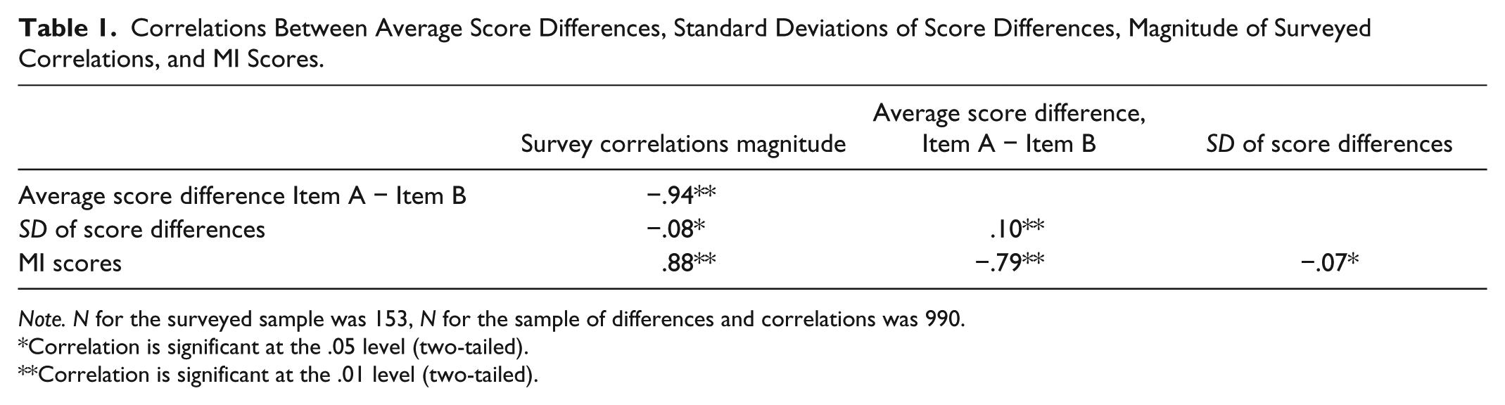
Note. N for the surveyed sample was 153, N for the sample of differences and correlations was 990.

*Correlation is significant at the .05 level (two-tailed).

Correlation is significant at the .01 level (two-tailed).

This provides a key to how MI values can allow us to estimate the value of a response to B if we know the response to A. MI scores can be translated into score distances because they are systematically related to the differences. By regressing the MI values on the score differences, the resulting standardized beta can be used to estimate the distance from A to B, given that we know A. Table 2 shows this regression. It displays a hierarchical model that enters the preadministration MI values in the first step. By also entering the postadministration in the second step, we supply additional support for the claim that these two sets of scores indeed contain the same information.

Table 2.

Hierarchical Regression Where MI Values (Step 1), Survey Correlations (Step 2) Were Regressed on the Average Score Differences (N = 990).

	Step 1	Step 2
MI values	−.79**	−.14**
Survey correlations	—	−1.07**
R ²	.63	.89
F	1,683.58	3,981.42

p < .01.

After entering the original surveyed correlations in Step 2, the beta for the MI values is substantially reduced, indicating that the information contained in the MI values is indeed isomorphic to the information in the survey correlations. The same table also shows how the information in MI values is slightly inferior to that of the correlations. This is to be expected, as the correlations and the standard deviations stem from the same source, while the MI algorithm is only one, imperfect algorithm out of several available choices. It has been shown elsewhere that it will usually take the output of several present-day algorithms to approximate the semantic parsing of natural human speakers (Arnulf et al., 2014), but improved algorithms may alleviate the problems in the future. Most importantly, we can use the beta of the first step to estimate a specific item response from knowledge about the MI value. In other words, we are training our respondent simulation algorithm using the regression equation above, capturing the beta as key to further computations.

Simulating Responses

Based on the consideration above, it is possible to hypothesize that a given respondent’s responses are not free to vary. Once the respondent has chosen a response to the initial items, the subsequent responses should be determined by the semantic relationships of the items (Arnulf et al., 2014; Nimon et al., 2016) and the structure of the survey, most notably the response categories (Maul, 2017; Slaney, 2017) and the unfolding patterns following from expected negative correlations (Michell, 1994; Roysamb & Strype, 2002; van Schuur & Kiers, 1994).

Ideally, it should be possible to predict any given response based on the knowledge of the semantic matrix and a minimum of initial responses. In our simulations, we can see that any response in the MLQ is predictable by using other known responses and knowledge about the distances between items. The R²s of these predictions are in the range of .86 to .94. As the semantic MI values correlate at –.79 and predict the distances significantly (R² = .63), it should theoretically be possible to substitute the distances with the semantic values, and thus predict later responses with a minimum of initial responses.

The perfect formula is yet to be found, but we have created a preliminary algorithm that can possibly mimic real responses to the MLQ. The present approach is explicitly aiming at reproducing existing responses as this gives us the best opportunity to compare simulated with real responses.

The rationale for the algorithm combines semantics and unfolding theory as follows:

Responses are restricted to the values 1 to 5 of the same Likert-type scale. The difference between any two items, A and B, within this Likert-type scale is here referred to as the “distance” between A and B; for example, if A is 5 and B is 4, the distance between them is 1 (5 − 4).

In the case of high MI values, Item B is likely to be very close to its preceding item, A. Lower MI values indicate higher and less determinate distances.

The most probable absolute distance between Item A and Item B is calculated as the MI value for A and B multiplied by the standardized beta in the regression equation of Table 2 (–0.79). To predict a given distance from this type of regression equation, the formula should be as follows: Value (Item B) = Constant + (MI for Item A and Item B) x – 0.79. However, the distances were computed as absolute measures; that is, the absolute distance from 3 to 5 = 2, but so is 5 to 3. In practice, though, the algorithm may need to predict a high number from a low number or vice versa. The constant will therefore not “anchor” the distance at the right point in the scale.

We therefore need to tie the estimated point to the value of Item A. We have tested several approaches to this, and the formula that seems to work best for calculating any response B is to simply replace the constant with the value for Item A, thus Value(Item B) = Value(Item A) + (MI for Item A and Item B) x − 0.79.

This formula does impose the structure of semantic values on the subsequent numbers. It also seems counterintuitive because if MI increases (indicating higher similarity), the term will grow in absolute numbers. However, the beta is negative, and the resulting number will be smaller. The impact on the ensuing calculations now comes from the unfolding operations, depending on whether Response B is higher or lower than A. To comply with predictions from unfolding theory, the formula above keeps its positive form if the respondent’s first three responses indicate a positive evaluation (biasing the item distances in a positive direction) but should be negative if the unfolding pattern appears to be negative. This information is picked up by comparing the responses of Items 1, 2, and 3. While Items 1 and 2 are descriptions of positive leadership, Item 3 contains a negative appreciation.

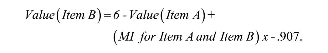
In the case that the Items A and B are assumed to be negatively related (this was discussed in the explanation of MI values above), the same relationship between MI and distances hold. However, the estimated value should logically be at the other end of the Likert-type scale (in a perfect negative correlation, a score of 5 on A indicates that the score for B is 1). So in the case of expected negative correlations, the direction of the algorithm formula is reversed within the 5-point Likert-type scale, such that

V a l u e (I t e m B) = 6 - V a l u e (I t e m A) + (M I f o r I t e m A a n d I t e m B) x - 0.79 .

In this way, it is possible to start with Item 1, and use the MI values to calculate the relationship of Item 1 to Items 2, 3, and so on until Item 45. This process is repeated for Item 2 to all Items 3 to 45 and so on, until all values have been calculated for all 990 unique pairs of items.

To simulate missing responses, we can now delete the original responses and replace them with those computed in Step 7 above.

One final requirement is theoretically and practically important. As mentioned, the MI values and correlations are not really distance measures, but a measure of uncertainty, which in cases of low MI values should be indeterminate. The formula used here instead applies the beta from the regression equation as a measure of distance. However, uncertain values are in turn restricted by having closer relationships to other items. The whole matrix of 990 unique pairs of items is comparable with a huge Sudoku puzzle where each item score is defined by its relationship to 44 other items. We can use this to smooth out the simulated values for each item by averaging all the 44 estimated values resulting from each of its 44 relationships.

In this way, our algorithm is based on the complete pattern of semantic distances for every item with all other items, as well as a hypothesis on the direction of scale unfolding based on the initial three responses. It is admittedly explorative and based on an incomplete understanding of the issues involved, and our intention is to invite criticism and improvements from others. One questionable feature of this algorithm is the tendency for positive evaluations to escalate positively and vice versa, probably due to a deficiency of the formula in Step 4. In the course of all 990 iterations however, these tendencies seem to balance each other out, and fix the averaged responses as dictated by the mutual pattern of semantic distances. We have also checked that this formula performs better than simply using averages of the known values instead of semantics, thus substantiating the use of semantics in the formula. A further contrasting procedure will be described below.

The MLQ has 45 items. Of these, 36 measure different types of leadership behaviors, and the nine last items measure how well the rated person’s work group does, commonly treated as “outcome” variables. The Arnulf et al. (2014) study found the “outcome” variables to be determined by the responses to the preceding items. We will therefore start by trying to predict the individual cases of these by deleting them from real response sets. By deleting progressive numbers of items, we will then explore how well the semantics will perform to predict the missing responses.

Therefore, our first simulated step will be concerned with predicting outcomes training the algorithm on the first 36 items. In the next steps, we simply subtract remaining half of the survey until all real responses are deleted, offering the algorithm diminishing amounts of training information. In this way, we can evaluate the degree to which the computed values still bear resemblance to the original values.

Contrast validation procedure

Algorithms like this may create artificial structures that are not due to the semantic MI values but simply artifacts created by the algorithm procedures themselves. To control for this, we have created similar sets of responses with the same numbers of missing values, where the MI values in the algorithm are replaced by randomly generated values in the same range as the MI values (from −1 to +1). If similarities between artificial and real responses are created by biases in the algorithmic procedure and not by semantics, the output of randomly generated numbers should also be able to reproduce numbers resembling the original scores. The difference between the output of random and semantically created numbers expresses the value of (present-day) semantics in predicting real responses.

Simulation Criteria

There are no previously tested criteria for assessing the quality of simulated survey responses compared with real ones. Survey data are generally used either as summated scores to indicate the respondents’ attitude toward the survey topic (score level or attitude strength) or as input to statistical modeling techniques such as structural equation modeling (SEM). In addition, survey data are often scrutinized by statistical methods to check their properties prior to such modeling (Nunnally & Bernstein, 2010). Therefore, we propose the following common parameters to evaluate the resemblance of the artificial responses to the real ones:

Scale reliability: The simulated scores should have acceptable reliability scores (Cronbach’s alpha), preferably similar to the real scores.

Accumulated scores: A simulated survey response should yield summated scale values similar to the ones of the surveyed population. Ideally, the average scores on simulated leadership scales should be nonsignificantly different from the average summated scores of real survey scores. The average, summated simulated scores should also be significantly different from the other scales (differential reliability).

Pattern similarity: The simulated survey scores should not only show similar magnitude, but the pattern of simulated scores should also correlate significantly with the real individual score profiles. In particular, there should be few or no negative correlations between real and simulated score profiles in a sample of simulated protocols.

Sample correlation matrix: The simulated scores should yield a correlation matrix similar to the one obtained from real survey scores.

Factor structure: The factor structure of simulated responses should bear resemblance to the factor structure emerging from the real sample.

Unfolding structure: Seen from the perspective of unfolding theory, extreme score responses are easier to understand than midlevel responses. In an extreme score, a positive respondent will have a general tendency to reject negative statements and endorse high positive scores, and a negative respondent will rank items in the opposite direction. Midlevel items across a complex scale would require more complex evaluations of how to “fold” each single item so as to stay with the dominant unfolding path (Michell, 1994). This is a tougher task for both respondents and the simulating algorithm. We therefore want to check if our algorithm is more appropriate for high and low than for medium scores.

Results

Table 3 shows the alpha values for all MLQ scales. Values for the real responses are in the first column. Computations are made for increasing numbers of missing values to the right. It can be seen that the alphas for simulated responses are generally better than those for the real responses (the alphas for simulated responses are lower for the simulated values in only six of 40 cases). The alphas generated from random semantic responses are inadequate and keep deteriorating as items are replaced by simulated responses.

Table 3.

Cronbach’s Alpha for All MLQ Scales, Real and Simulated Responses.

	Real	Outcome items missing	21 (46%) items missing	33 (73%) items missing	33 items random semantics	39 (86%) items missing	39 items random semantics	42 (95%) items missing	42 items random semantics	100% synthetic
Idealized influence attr	.74	.77	.82	.88	−.10	.99	.13	1.00	−.15	.99
Idealized influence beh	.72	.72	.72	.90	−.07	.92	−.04	.99	−.06	.99
Inspiring motivation	.80	.80	.82	.91	.09	.99	−.12	1.00	−.05	.99
Intellectual stimulation	.83	.82	.84	.85	.45	.91	−.20	.93	−.11	.76
Indvidualized consider.	.78	.78	.82	.99	−.22	1.00	.16	1.00	−.06	.99
Conditional reward	.73	.73	.79	.90	.42	.99	.10	1.00	−.20	.99
Mgmnt by exception act.	.51	.52	.43	.72	.00	.77	.13	.97	−.27	.95
Mgmnt by exception pas.	.47	.47	.47	.76	.38	.82	−.09	.83	−.06	.83
Laissez-faire	.77	.77	.75	.78	.33	.84	−.03	.99	−.07	.97
Outcome measures	.92	1.00	1.00	1.00	.18	1.00	−.02	1.00	.07	1.00

Note. MLQ = Multifactor Leadership Questionnaire.

Table 4 shows the mean summated scores for each of the MLQ subscales in the sample. When the nine outcome measures are missing (replaced by simulated scores), their simulated scale is nonsignificantly different from the original. When 21 item scores are missing (46% missing), there are only two instances of significant scale differences. When 33 or 39 items are missing, the number of significant differences increases, but the average differences from the real scores are very small: 0.08 Likert-type scale points even for the 35 missing items, and 0.18 points in difference where 39 items (86% of the responses) are missing and replaced by simulated scores. Most of the scales are also still significantly different from each other, such that no scale measuring transformational leadership overlaps with Laissez-Faire, Passive Management by Exception, or outcome variable scores. There is a tendency for some of the differences between the scales within the transformational leadership construct to overlap with increasing number of simulated items.

Table 4.

Means for Subscales by Simulated Populations.

Main constructs	Real	Outcome items missing	21 (46%) items missing	33 (73%) items missing	33 items random semantics	39 (86%) items missing	39 items random semantics	42 (95%) items missing	42 items random semantics
IdealizedAttrib	3.43	3.42	3.39	3.58	3.03	3.79	3.02	3.87	3.00
IdealizedBehv	3.94	3.95	3.84	3.78	3.23	3.86	3.22	3.83	2.98
InspMotive	3.83	3.84	3.78	3.77	3.23	3.78	3.00	3.86	2.99
IntellStim	3.28	3.28	3.44	3.55	3.14	3.63	3.06	3.69	3.06
IndConsid	3.59	3.59	3.59	3.73	3.01	3.84	3.00	3.90	3.02
CondReward	3.79	3.79	3.71	3.80	3.44	3.84	3.27	3.90	3.23
MBEact	3.06	3.08	3.11	3.63	3.06	3.70	3.06	3.78	2.97
MBEpass	2.63	2.62	2.62	2.38	2.73	2.39	2.98	2.33	2.98
LaissFaire	2.37	2.37	2.43	2.32	2.71	2.28	2.85	2.22	3.01
Outcome	3.53	3.59	3.69	3.85	3.00	3.91	3.00	3.94	2.99
Average difference from real		.01	.07	.20	.38	.25	.47	.30	.52

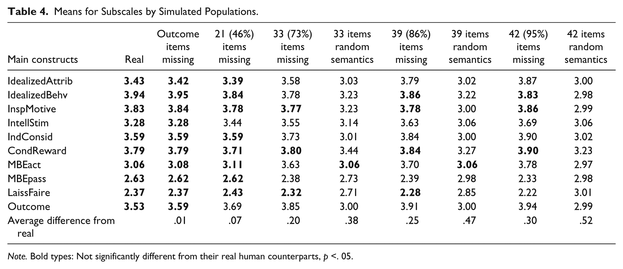
Note. Bold types: Not significantly different from their real human counterparts, p <. 05.

When all these scores are summed up in their purported higher level constructs—transformational, transactional, laissez-faire leadership and outcomes, this pattern of average scores is maintained. Scores computed with random semantics depart quicker and more dramatically from their real counterparts, see Table 5.

Table 5.

Means for Main Constructs by Simulated Populations.

Main constructs	Real	Outcome items missing	21 (46%) items missing	33 (73%) items missing	33 items random semantics	39 (86%) items missing	39 items random semantics	42 (95%) items missing	42 items random semantics
Transformational	3.62	3.62	3.61	3.68	3.13	3.78	3.06	3.83	3.01
Transactional	3.16	3.16	3.15	3.27	3.07	3.31	3.10	3.34	3.06
Laissez-faire	2.37	2.37	2.43	2.32	2.71	2.28	2.85	2.22	3.01
Outcomes	3.53	3.59	3.69	3.85	3.00	3.91	3.00	3.94	2.99
Average difference from real		.02	.06	.14	.36	.20	.41	.24	.47

Note. Bold types: Not significantly different from their real human counterparts, p <. 05.

Every individual’s simulated responses were correlated with their real counterparts to compare the pattern of real versus simulated responses. Table 6 shows how these correlations were distributed in the various simulated groups. As could be expected, there is a decline in the resemblance between the simulated scores and their real duals as the number of simulated scores increases. However, this decline happens much faster for the scores generated by random patterns, and when 43 items are replaced with simulated scores, there are still only eight cases (5%) that correlate negatively with the real respondents, see Figure 1.

Table 6.

Characteristics of the Average Correlations Between Real and Simulated Respondents by Number of Simulated Item Responses.

Scale	No of negative correlations	Minimum correlation	Maximum correlation	Mean correlation	SD
Outcome items (nine) missing	0	.79	1.00	.94	.05
21 items missing	0	.35	1.00	.83	.10
33 items missing	0	.06	.91	.61	.18
33 items random semantics	0	.11	.81	.50	.11
39 items missing	2	−.24	.87	.34	.31
39 items random semantics	2	–.08	.57	.31	.11
42 items missing	8	−.62	.88	.44	.29
42 items random semantics	22	–.26	.42	.14	.13

Figure 1.

The frequency distribution of correlations between real and stimulated responses for the simulated populations, replacing 42 of 45 item responses with simulated scores.

We explored how the relationships among the subscales of the MLQ changed with increasing numbers of missing items. An interesting difference appeared between the values replaced by the semantically informed algorithm and the algorithm with random semantic values: With increasing numbers of simulated values, the correlations among the subscales tended to increase for the semantically informed simulations. Where the semantic predictions were replaced by random numbers (leaving only the pattern of the algorithm itself, void of semantics), the correlations among the subscales decreased, approaching 0 where 39 of 45 responses were simulated, see Figure 2.

Figure 2.

Absolute interscale correlations by simulated sample.

We then performed a principal components analysis (PCA) on these samples to compare their ensuing patterns. The MLQ has been criticized for its messy factor structure over the years, as some people find support for it and others do not (Avolio et al., 1995; Schriesheim, Wu, & Scandura, 2009; Tejeda, Scandura, & Pillai, 2001). In our sample here (N = 153), there emerged eight or nine factors, but the rotated factors were not clearly delineated and did not fully support the theorized structure of the survey. However, we are here not concerned with the structure of the MLQ itself but with the similarity of the real and simulated measures. Table 7 shows that as an increasing number of items are replaced by semantically simulated ones, there is a gradual reduction in the number of factors identified. This is completely opposite from what happens where scores are computed with random input to the algorithm. In these cases, there is a proliferation of eigenvalues increasing with the numbers of simulated variables. The numbers of factors indicated by scree plots are displayed in brackets as these may be just as interesting as factors identified by eigenvalues (see Figure 3). The MI values seem to impose a simplified structure on the data in PCA reminiscent of factor structures, and rotational procedures did not change the emerging patterns. The two factors emerging from the purely synthetic condition seem to be an artifact of the algorithm because it needs two (randomly chosen) initial values to get started.

Table 7.

Number of Factors With Eigenvalue >1 Extracted in Principal Components Analysis, Real and Simulated Samples (Factors Indicated by Scree Plots in Brackets).

	Real	Outcome items missing	21 items missing	33 items missing	33 items random semantics	39 items missing	39 items random semantics	42 items missing	42 items random semantics	Synthetic
Computed on all 45 items	9 (4)	8 (4)	6	4	19	3 (5)	18	2 (3)	30	2 (3)
Computed without outcome items	8 (4)	8 (4)	6	4	16	3 (6)	15	2 (3)	16	2 (3)

Figure 3.

Principal components scree plots, one real and three simulated samples (39 times missing, 39 items replaced with random semantics, one completely synthetic sample).

We finally checked whether the score levels could affect the similarity between simulated and real responses. As we were expecting, higher scores of both transformational leadership and laissez-faire (and, by implication, the outcome values) were all related to higher correlations between the real response and its simulated duplicate. This tendency was increasing for a higher number of simulated scores but absent in responses computed in the random control condition, see Table 8.

Table 8.

The Relationship Between Magnitude of Correlation Between Subscale Score Levels, and the Relationships Between Real and Simulated Response by Number of Simulated Items.

MLQ subscale	Outcome (nine) items missing	21 items missing	33 items missing	33 missing random semantics	39 items missing	39 missing, random semantics	42 item missing	42 missing, random semantics
Transform.	.46**	.50**	.50**	−.05	.27**	−.02	.59**	.02
Transact.	.15	.12	.23**	−.13	.14	−.13	.54**	.04
Laissez-faire	−.36**	−.53**	−.51**	−.23**	−.28**	−.19*	−.60**	.02
Outcomes	.45**	.43**	.41**	.00	.26**	−.06	.57**	.12

Note. MLQ = Multifactor Leadership Questionnaire.

p < .05 level (two-tailed). **p < .01 level (two-tailed).

Discussion of Study 1

Summing up our findings, the following descriptions seem supported:

Outcome measures: When the outcome measures were substituted with simulated measures, these were virtually nondistinguishable from the real measures. This implies that the purported outcome variables are not independent and empirical but determined directly by the semantic relationships to the previous survey items. The simulated outcome levels were nondistinguishable from the real ones even when 39 of 45 items were replaced by simulated items.

Reliability: The reliability levels of scales in the simulated responses were comparable with and in most cases better than the real responses. With increasing numbers of items substituted by simulated items, the alpha values increased. Responses computed with random semantic figures presented deteriorating alphas. This supports our claim that the psychometric structures are caused by the semantic patterns and are not an artifact of the algorithm.

Summated scale levels: Even with the simple algorithm applied here, six real item responses (of 45 scale items) are enough to predict the level of transformational leadership and laissez-faire scale scores precisely. Twelve items allow a fairly precise calculation of the summated level of each of the 10 subscales. The respondents’ levels of endorsing or criticizing their managers’ leadership behaviors were reliably captured by a small subset of items. When the computed composite scores started deviating in a statistically significant way from the real score levels, the differences were still quite small, and with the exception of the scale Passive Management By Exception, they were always closer to the real ones than to the randomly generated scores.

Pattern similarity: The simulated survey responses were correlating highly with their real origins, and there were almost no cases where these correlations took negative values. That is interesting, given Michell’s (1994) findings that only a few percentage of survey respondents will respond in a way that violates the semantic structure of the survey and its unfolding pattern. Even the sample computing 42 simulated scores from three given responses was highly and significantly correlated with their real counterparts. It seems warranted to say that the pattern of scores created by our simulation algorithm largely replicated the pattern of real responses. The randomly generated patterns performed clearly inferior to the true semantic values.

Correlation matrices: For the sake of brevity, we compared only the correlation matrices of the accumulated subscales, substituting real scores for samples with increasing numbers of simulated responses. This comparison is probably the one where simulated scores did not perform so well. The correlations among the scales were increasing with increasing numbers of simulated responses. This finding is however mixed in terms of STSR relevance: While our algorithm seems to be less sensitive to differential information with more simulated items, the correlations will tend to increase in magnitude. This means that all else being equal, semantic information is a powerful source of correlations in survey data. This was evident in comparison with the correlation matrices generated from random values, which were approaching 0 as more responses were replaced by simulated ones.

Factor structure: As with the correlation matrices (and related to this matter), the factor structures of the data samples were increasingly simple with more semantics based on simulated scores, ending with a two-factor model when all but three items were computed (95% of the items replaced). The MLQ may not be a good testing ground for factor structures, as it was itself quite messy in the small random sample we used here. Still, the sample using simulated outcome scores identified the outcomes as clearer than the real sample did. Random responses developed in the opposite direction and quickly began generating extra factors proliferating upward to 15 to 30 factors.

Unfolding structure: As we expected, the simulator was most accurate in recreating response patterns at the extreme score level; that is, respondents who were very negative or very positive toward their managers. Intermediate levels were harder to simulate exactly, and the scale “Active management by exception” seems in all explorations to offer the least precisely estimated scores by our algorithm. This difficulty handling the “lukewarm” scores is expected from unfolding theory (Andrich, 1996; Coombs, 1964; Coombs & Kao, 1960; Michell, 1994; Roberts, 2008) because such intermediate response patterns give rise to more complex folding of scales.

Study 2

Measures

The scale subjected to simulation of scores here is a composite of three scales frequently used in OB research: Two scales published measuring perceptions of economic and social exchange, comprising eight and seven items, respectively (Shore, Tetrick, Lynch, & Barksdale, 2006), and one scale measuring intrinsic motivation comprising five items (Kuvaas, 2006). These scales were chosen because they originate from different researchers and have not been part of a coherent instrument. They are also shorter and offer less complexities than the MLQ. These scales displayed semantic predictability in the previous study on STSR (Arnulf et al., 2014).

Sample

A randomly chosen sample of 100 employees from a Norwegian governmental research organization was used to train and validate the algorithm. About 72% of the respondents were male, and the majority of respondents were holding university degrees at bachelor level or higher.

Analytical Procedures

We used the MI algorithm to compute semantic similarities between all 20 items. This yields a matrix of 20 × 19 / 2 = 190 unique item pairs. The problem of negatives was solved as described in the case of the MLQ, as the scale measuring economic exchanged can be shown a priori to be negatively correlated with the other two (see Arnulf et al., 2014). Also, one item measuring social exchange is originally reversed, and kept that way to conform with the theoretical handling of negatives.

The semantic indices from the MI algorithm predicted the sample correlation matrix significantly with an adjusted R² of .52. As in the study above, this relationship was even stronger with the interitem distances (the average distance in scores between Item A and Item B . . . ), reaching an adjusted R² of .81. To train the predicting algorithms, we kept the constant (1.342) and unstandardized beta (–.907) from the latter regression analysis.

Individual response patterns were predicted by applying the algorithm developed in Study 1. We replaced the sample constant and unstandardized beta with the values from this sample, tested this version first:

For predicted positive correlations,

V a l u e (I t e m B) = V a l u e (I t e m A) + (M I f o r I t e m A a n d I t e m B) x - . 907 .

For predicted negative correlations,

V a l u e (I t e m B) = 6 - V a l u e (I t e m A) + (M I f o r I t e m A a n d I t e m B) x - . 907 .

The resulting numbers were promising but did not seem totally satisfactory, possibly due to unfolding problems. Whereas the MLQ is composed of highly heterogeneous subscales distributed in a mixed sequence, the Study 2 scales are very homogeneous and distributed one by one. It is hard to find an a priori rule for the unfolding of the combined scale. However, the unstandardized beta is –.907 which is almost −1, and so plays a small role when multiplied with other values except changing the sign. We first removed the sign to check the effect on unfolding, but results were equally promising but unsatisfying. We then decided to remove the beta and replace it with the constant for the item differences instead (1.342) plus the semantic MI value. This provided a better approximation of the scores:

For predicted positive correlations,

V a l u e (I t e m B) = V a l u e (I t e m A) + (M I f o r I t e m A a n d I t e m B) + 1.342 .

For predicted negative correlations,

V a l u e (I t e m B) = 6 - V a l u e (I t e m A) + (M I f o r I t e m A a n d I t e m B) + 1.342 .

We then proceeded to explore if the responses simulated from semantic values predict their “real” counterparts better than random values in the same range (control condition).

Results

The results will be reported summarily along the same lines as in Study 2:

Summated scale levels: Figure 4 shows the average accumulated scores for three test samples. The patterns of the semantically simulated scores are similar to the real sample, but the average score on intrinsic motivation is somewhat low (albeit significantly higher than the score for social exchange). Adjusting the unfolding pattern in the algorithm could possibly alleviate this. Importantly, the pattern seemed driven by the semantic values, as the random values tend to wipe out the pattern and the average scores become similar.

Pattern similarity: The semantically simulated test responses correlated on average .56 with the originals. The highest correlation was .89 and the lowest was –.37, but only two of the 100 simulated responses correlated actually negatively with their real counterparts. The simulations using random semantics yielded an average correlation of .10 with 30% negative correlations.

Reliability: The simulated responses yielded an α of 1.00, α for the random semantics was .99, and α for the real sample was .79.

Factor structure: The 20 items were subjected to PCA with varimax rotation. The real responses yielded five factors explaining 65.5% of the variation. The responses simulated with semantic values yielded two factors explaining 98%, and the random semantics also produced two factors explaining 99%. A more interesting picture emerges when presenting two-dimensional plots of the factor structures, as displayed in Figure 5.

Figure 4.

Average scale scores for the three scales for semantically simulated, real respondents and random semantics.

Figure 5.

Factor structures of random, semantic, and real samples.

The two-dimensional plots reveal that the random semantics cannot distinguish between the three scales. The real sample produces three distinct clusters even if it does not present a satisfactory solution. The simulated sample presents a clear three-factor plot of the items. The reversed item in the social exchange scale is plotted on the same axis but orthogonally to the nonreversed, as theoretically expected. Still, social exchange items were erroneously grouped with intrinsic motivation.

Unfolding structure: As in Study 1, there was a clear relationship between the semantic predictability of the individual response patterns and their score levels. The simulated response patterns correlated at .67 with the dispersion of scores (standard deviation of scores within the individual) and .57 with the score level on intrinsic motivation (p < .01). Elevated scores increase the score dispersion, allowing the responses to be more predictable.

Discussion of Study 2

As in Study 1, the semantically simulated responses were similar but not completely identical to the original responses that they were meant to predict.

Simulated scales were similar in the sense that (a) the aggregated means of the main variables were of similar magnitude and exhibited similar mutual patterns, (b) the reliabilities were high or higher than the originals, (c) the majority of the simulated response patterns correlated highly with the original patterns with only 2% in a negative direction, and (d) the factor structure in PCA indicated a three-factor solution but only in a two-dimensional plot.

The simulated responses failed to produce a level of intrinsic motivation as high as the original (higher than the two other scales but significantly lower), and the factor structure failed to reproduce three clear-cut factors.

On the contrary, the simulated scores created with random semantics failed to replicate the originals on all accounts except for the alphas. This indicates that key characteristics of survey data—score levels, factor structures, and variable relationships—were reproducible by means of semantic indices in these scales.

Also, the three scales did not emerge clearly from the real responses. The present dataset may not have been ideal for training simulation algorithms. For the sake of brevity, we do not report the systematic effect of deleting real responses in Study 2.

Final Discussion and Suggestions for Future Research

The main purpose of this article was to develop and apply a simple algorithm for creating artificial responses, and compare these with a sample of real responses, explaining the rationale behind STSR and opening a field of exploring survey responses through computation. Across two different scales and samples, we were able to check the psychometric properties of simulated scores compared with the real human responses. The semantic indices always performed much better in predicting real scores than random numbers in the same range.

This is a new field with no established quality criteria, and so our aim was simply to conduct a test applying what we know. We also want to be transparent about what we do, omitting overly complicated steps that could have improved the performance.

The results could partly be artifacts of the algorithm itself. As we have pointed out, research on the effects of unfolding and measurements in construct validation has repeatedly shown that the survey structure itself is a major source of systematic variation, and hence needs to be considered in predicting responses (Maul, 2017; Michell, 1994; Slaney, 2017; van Schuur & Kiers, 1994).

However, we do think that improvements in predicting real scores are foreseeable already, addressing the following series of issues:

A theoretically more precise formula: It should ideally be possible to formulate a mathematically rigorous way to translate the semantic matrix into the distance matrix, and from the distance matrix to a prediction of Item B if Item A is known. This is the main theoretical goal of STSR, and we are not yet there.

More precise semantic estimates: This study applied semantics from the MI algorithm only. It is shown elsewhere that a combination of semantic algorithms will have incremental explanatory power (Arnulf & Larsen, 2015; Arnulf et al., 2014). Also, other computational methods have been shown to produce similar results and could possibly be combined with what we do here (Gefen & Larsen, 2017; Nimon et al., 2016). More advanced combinations of semantic values in the model may allow more precise replications of real responses.

A more precise weighting measure: In Study 1, we consequently used the beta from a model where the semantic values are regressed on the observed score differences. This was used as a benchmark to translate from MI values into probable score distances because it could be justified fairly simply. Study 2 showed that using the constant yielded better results. A more systematic mathematical rationale could create scores that are less uniform in the way they impose structure on the data, and could possibly keep the factor structure intact as produced by humans. One possibility is to replace the distance approximation with a probability function that could add some random error to the formula.

A better model for unfolding of the items: The unfolding pattern we created in Study 1 was also just a quick rule of thumb, and in Study 2, we did not take the unfolding into account at all, except for the negative correlations. More differentiated unfolding patterns could be modeled. One way would be to include more knowledge from the initial training data. This could increase the variation in data and reduce the tendency toward simplification of structures, as well as improving the performance of the algorithm in responses with medium-range responses. An important question to address is the case of multidimensional scales as in our second dataset. In such cases, it may be necessary to fix the response level for each dimension, which points to the entry of nonsemantic information about attitude strength in the data.

More advanced smoothing function: The fact that all items are locked in a grid of differing relationships to 44 other items is intriguing. A mathematical procedure that could capture this complex network of values would be a much more direct approach to calculations, possibly akin to multidimensional scaling (Borg & Groenen, 2005). This could let us test the degree to which people create response patterns deviating from what is semantically given. Not only would it inform STSR and unfolding theory but also allow us to differ better between empirical questions (pertaining to how people actually respond) and logical questions (setting up conditions for how people ideally should respond; Semin, 1989; Smedslund, 1988).

The results seem to support our main theoretical proposition to some degree. To the extent that survey responses are semantically determined, they are predictable a priori.

The semantic values generally produced high alphas, high correlations, and orderly patterns in the data, which the randomly generated semantic values failed to produce even if the other steps of the algorithm were identical in both sets of simulated responses. An alarming finding in our data is that the semantic structure seems to produce better alphas and factor structures, possibly leading researchers to lean toward semantics in scale constructions to comply with current guidelines for fit indices (Hu & Bentler, 1999).

In STSR, survey responses may be seen more as an expression of coherent beliefs than a series of quantitative responses. The initial responses signal the endorsement of opinions. These could have been semantically explicit specifications of the response alternatives as in, for example, Guttman scales (Michell, 1994). “Response strength” may be seen as a signal carrier for the semantic anchor of the respondent’s interpretation of the items.

In this regard, it is important to distinguish between survey responses as an individual expression and the survey responses as input to aggregated sample statistics. STSR cannot predict the initial response level of a given respondent a priori, the “theta” in item response theory (Singh, 2004). What the theory predicts is that once the individual’s level is set, the patterns (or values) of the remaining items are influenced or even determined by their semantic structure. Their values are not free to vary because they share overlapping meaning, and therefore share the same subjective evaluation. Thus, it will be the semantically determined patterns that carry over into the sample statistics, not so much the attitude strength (Arnulf, Larsen, Martinsen, & Egeland, 2018).

Sample statistics—the bulk of the correlations in the MLQ—may therefore be determined by semantic relationships that are void of attitude strength. This allows a precise prediction of the “outcome” scales by semantics as demonstrated above and theoretically predicted by others (Van Knippenberg & Sitkin, 2013).

Taken together, our preliminary outline of a simulation procedure indicates how simulating semantically expected scores is possible. Subsequently, this may allow us to explore how to depart from what is semantically expected instead of rediscovering semantically predetermined relationships.

STSR does not propose that all survey data come about as a result of semantics. Neither does the theory claim that this model holds across all constructs. STSR simply proposes that whatever the sources of variation in survey data, the semantics implied is the first source to evaluate, often more powerful and systematic than hitherto assumed. By offering a rationale and an outline for experimental research on STSR, we hope future developments can address more detailed questions of the nature and interaction of survey response.

Footnotes

Declaration of Conflicting Interests

The author(s) declared no potential conflicts of interest with respect to the research, authorship, and/or publication of this article.

Funding

The author(s) disclosed receipt of the following financial support for the research, authorship, and/or publication of this article: We thank the U.S. National Science Foundation for research support under Grant NSF 0965338 and the National Institutes of Health through Colorado Clinical & Translational Sciences Institute for research support under NIH/CTSI 5 UL1 RR025780.

ORCID iD

Jan Ketil Arnulf

Author Biographies

Jan Ketil Arnulf, PhD, is an associate professor at BI Norwegian Business School, teaching and researching leadership and leadership development. He has served as an associate dean to the BI-Fudan MBA program in Shanghai, China.

Kai R. Larsen, PhD, is an associate professor of management and entrepreneurship at Leeds Business School, University of Colorado at Boulder. He serves as the director of the federally supported Human Behavior Project, researching a transdisciplinary “backbone” for theoretical research. He teaches business intelligence and privacy in the age of Facebook.

Øyvind L. Martinsen, PhD, is a full professor at BI Norwegian Business School in Oslo, Norway. He conducts research in leadership, personality, and creativity, and also teaches these issues as well as psychometrics.

References

Abdi

(2003). Factor rotations in factor analysis. In Lewis-Beck

Bryman

Futing

(Eds.), Encyclopedia of social sciences research methods (pp. 792-795). Thousand Oaks, CA: Sage.

Andrich

(1996). A hyperbolic cosine latent trait model for unfolding polytomous responses: Reconciling Thurstone and Likert methodologies. British Journal of Mathematical and Statistical Psychology, 49, 347-365.

Arnulf

J. K.

Larsen

K. R.

(2015). Overlapping semantics of leadership and heroism: Expectations of omnipotence, identification with ideal leaders and disappointment in real managers. Scandinavian Psychologist, 2, e3. doi:10.15714/scandpsychol.2.e3

Arnulf

J. K.

Larsen

K. R.

Martinsen

Ø. L.

Egeland

(2018). The failing measurement of attitudes: How semantic determinants of individual survey responses replace measures of attitude strength. Behavior Research Methods, 1-21. doi:10.3758/s13428-017-0999-y

Arnulf

J. K.

Larsen

K. R.

Martinsen

Ø. L.

Bong

C. H.

(2014). Predicting survey responses: How and why semantics shape survey statistics in organizational behavior. PLos ONE, 9(9), e106361. doi:10.1371/journal.pone.0106361

Avolio

B. J.

Bass

B. M.

Jung

D. I.

(1995). Multifactor Leadership Questionnaire technical report. Redwood City, CA: Mind Garden.

Bagozzi

R. P.

(2011). Measurement and meaning in information systems and organizational research: Methodological and philosophical foundations. MIS Quarterly, 35, 261-292.

Borg

Groenen

(2005). Modern multidimensional scaling: Theory and applications (2nd ed.). New York, NY: Springer.

Borsboom

(2008). Latent variable theory. Measurement, 6, 25-53.

10.

Borsboom

(2009). Educational measurement: Book review. Structural Equation Modeling, 16, 702-711. doi:10.1080/10705510903206097

11.

Coombs

C. H.

(1964). A theory of data. New York, NY: Wiley.

12.

Coombs

C. H.

Kao

R. C.

(1960). On a connection between factor analysis and multidimensional unfolding. Psychometrika, 25, 219-231.

13.

Feldman

J. M.

Lynch

J. G. J.

(1988). Self-generated validity and other effects of measurement on belief, attitude, intention, and behavior. Journal of Applied Psychology, 73, 421-435.

14.

Firmin

M. W.

(2010). Commentary: The seminal contribution of Richard LaPiere’s attitudes vs actions (1934) research study. International Journal of Epidemiology, 39, 18-20. doi:10.1093/ije/dyp401

15.

Gefen

Larsen

K. R.

(2017). Controlling for lexical closeness in survey research: A demonstration on the technology acceptance model. Journal of the Association for Information Systems, 18, 727-757.

16.

Habing

Finch

Roberts

J. S.

(2005). A Q3 statistic for unfolding item response theory models: Assessment of unidimensionality with two factors and simple structure. Applied Psychological Measurement, 29, 457-471. doi:10.1177/0146621604279550

17.

Bentler

P. M.

(1999). Cutoff criteria for fit indexes in covariance structure analysis: Conventional criteria versus new alternatives. Structural Equation Modeling, 6, 1-55.

18.

Jöreskog

K. G.

(1993). Testing structural equation models. In Bollen

K. A.

Long

J. S.

(Eds.), Testing structural equation models (pp. 294-316). Newbury Park, CA: Sage.

19.

Kuvaas

(2006). Work performance, affective commitment, and work motivation: The roles of pay administration and pay level. Journal of Organizational Behavior, 27, 365-385.

20.

Lamiell

J. T.

(2013). Statisticism in personality psychologists’ use of trait constructs: What is it? How was it contracted? Is there a cure? New Ideas in Psychology, 31, 65-71. doi:10.1016/j.newideapsych.2011.02.009

21.

LaPiere

R. T.

(1934). Attitudes vs. actions. Social Forces, 13, 230-237.

22.

Leacock

Miller

G. A.

Chodorow

(1998). Using corpus statistics and WordNet relations for sense identification. Computational Linguistics, 24, 147-165.

23.

Likert

(1932). A technique for the measurement of attitudes. Archives of Psychology, 140, 1-55.

24.

MacKenzie

S. B.

Podsakoff

P. M.

Podsakoff

N. P.

(2011). Construct measurement and validation procedures in MIS and behavioral research: Integrating new and existing techniques. MIS Quarterly, 35, 293-334.

25.

Maul

(2017). Rethinking traditional methods of survey validation. Measurement: Interdisciplinary Research and Perspectives, 15, 51-69. doi:10.1080/15366367.2017.1348108

26.

Michell

(1994). Measuring dimensions of belief by unidimensional unfolding. Journal of Mathematical Psychology, 38, 244-273.

27.

Michell

(2013). Constructs, inferences, and mental measurement. New Ideas in Psychology, 31, 13-21. doi:10.1016/j.newideapsych.2011.02.004

28.

Mihalcea

Corley

Strapparava

(2006). Corpus-based and knowledge-based measures of text semantic similarity. American Association for Artificial Intelligence, 6, 775-780.

29.

Miller

(1995). WordNet: A lexical database for English. Communications of the ACM, 38(11), 39-41. doi:10.1145/219717.219748

30.

Mohler

Mihalcea

(2009, March 30-April 03). Text-to-text semantic similarity for automatic short answer grading. Paper presented at the 12th Conference European Chapter of the Association for Computational Linguistics (EACL 2009), Athens, Greece.

31.

Nimon

Shuck

Zigarmi

(2016). Construct overlap between employee engagement and job satisfaction: A function of semantic equivalence? Journal of Happiness Studies, 17, 1149-1171. doi:10.1007/s10902-015-9636-6

32.

Nunnally

J. C.

Bernstein

I. H.

(2010). Psychometric theory (3rd ed.). New York, NY: McGraw-Hill.

33.

Ortiz de Guinea

Titah

Léger

P.-M.

(2013). Measure for measure: A two study multi-trait multi-method investigation of construct validity in IS research. Computers in Human Behavior, 29, 833-844.

34.

Podsakoff

P. M.

MacKenzie

S. B.

Podsakoff

N. P.

(2012). Sources of method bias in social science research and recommendations on how to control it. In Fiske

S. T.

Schacter

D. L.

Taylor

S. E.

(Eds.), Annual review of psychology (Vol. 63, pp. 539-569). Palo Alto, CA: Annual Reviews.

35.

Poli

Healy

Kameas

(2010). WordNet. In Fellbaum

(Ed.), Theory and applications of ontology: Computer applications (pp. 231-243). New York, NY: Springer.

36.

Roberts

J. S.

(2008). Modified likelihood-based item fit statistics for the generalized graded unfolding model. Applied Psychological Measurement, 32, 407-423. doi:10.1177/0146621607301278

37.

Roysamb

Strype

(2002). Optimism and pessimism: Underlying structure and dimensionality. Journal of Social & Clinical Psychology, 21, 1-19.

38.

Rubin

D. B.

(1987). Multiple imputation for nonresponse in surveys. New York, NY: Wiley.

39.

Schriesheim

C. A.

J. B.

Scandura

T. A.

(2009). A meso measure? Examination of the levels of analysis of the Multifactor Leadership Questionnaire (MLQ). The Leadership Quarterly, 20, 604-616. doi:10.1016/j.leaqua.2009.04.005

40.

Schwarz

(1999). Self-reports: How the questions shape the answers. American Psychologist, 54, 93-105.

41.

Semin

(1989). The contribution of linguistic factors to attribute inferences and semantic similarity judgements. European Journal of Social Psychology, 19, 85-100.

42.

Shore

L. M.

Tetrick

L. E.

Lynch

Barksdale

(2006). Social and economic exchange: Construct development and validation. Journal of Applied Social Psychology, 36, 837-867.

43.

Singh

(2004). Tackling measurement problems with item response theory: Principles, characteristics, and assessment, with an illustrative example. Journal of Business Research, 57, 184-208. doi:10.1016/s0148-2963(01)00302-2

44.

Slaney

K. L.

(2017). Validating psychological constructs: Historical, philosophical, and practical dimensions. London, England: Palgrave Macmillan.

45.

Slaney

K. L.

Racine

T. P.

(2013a). Constructing an understanding of constructs. New Ideas in Psychology, 31, 1-3. doi:10.1016/j.newideapsych.2011.02.010

46.

Slaney

K. L.

Racine

T. P.

(2013b). What’s in a name? Psychology’s ever evasive construct. New Ideas in Psychology, 31, 4-12. doi:10.1016/j.newideapsych.2011.02.003

47.

Smedslund

(1988). What is measured by a psychological measure? Scandinavian Journal of Psychology, 29, 148-151.

48.

Tejeda

M. J.

Scandura

T. A.

Pillai

(2001). The MLQ revisited: Psychometric properties and recommendations. The Leadership Quarterly, 12, 31-52. doi:10.1016/S1048-9843(01)00063-7

49.

Van Knippenberg

Sitkin

S. B

. (2013). A critical assessment of charismatic-transformational leadership research: Back to the drawing board? The Academy of Management Annals, 7, 1-60. doi:10.1080/19416520.2013.759433

50.

van Schuur

W. H.

Kiers

H. A. L

. (1994). Why factor analysis often is the incorrect model for analyzing bipolar concepts, and what models to use instead. Applied Psychological Measurement, 18, 97-110.

Respondent Robotics: Simulating Responses to Likert-Scale Survey Items

Abstract

Keywords

Introduction

Theory

Semantics and Correlations

Study 1

Sample

Estimating Item Semantics

Semantics and Survey Correlations

Simulating Responses

Contrast validation procedure

Simulation Criteria

Results

Discussion of Study 1

Study 2

Measures

Sample

Analytical Procedures

Results

Discussion of Study 2

Final Discussion and Suggestions for Future Research

Footnotes

Declaration of Conflicting Interests

Funding

ORCID iD

Author Biographies

References