
Abstract
In the context of population aging, the U.K. government is encouraging people to work longer and delay retirement, and it is claimed that many people now make “gradual” transitions from full-time to part-time work to retirement. Part-time employment in older age may, however, be largely due to women working part-time before older age, as per a U.K. “modified male breadwinner” model. This article therefore separately examines the extent to which men and women make transitions into part-time work in older age, and whether such transitions are influenced by marital status. Following older men and women over a 10-year period using the English Longitudinal Study of Ageing, this article presents sequence, cluster, and multinomial logistic regression analyses. Little evidence is found for people moving into part-time work in older age. Typically, women did not work at all or they worked part-time (with some remaining in part-time work and some retiring/exiting from this activity). Consistent with a “modified male breadwinner” logic, marriage was positively related to the likelihood of women belonging to typically “female employment pathway clusters,” which mostly consist of part-time work or not being employed. Men were mostly working full-time regardless of marital status. Attempts to extend working lives among older women are therefore likely to be complicated by the influence of traditional gender roles on employment.
Introduction
Aging populations in many advanced countries, combined with a trend toward early exits from the labor market, have put pressure on current pension schemes (Fasang, 2009) and have led to pension reforms in many industrialized countries (Taylor, 2013) including the United Kingdom (Lain & Vickerstaff, 2014). Early exits from the labor market are seen as problematic, and as a result, the U.K. government is promoting extended working lives (Lain & Vickerstaff, 2015; Weyman, Wainwright, O’Hara, Jones, & Buckingham, 2012). This includes initiatives to equalize male and female state pension ages to 65, and then to raise them to age 68 and beyond (Lain, 2016). Likewise, mandatory retirement was abolished for most workers in 2011, theoretically enabling individuals to choose to work beyond age 65 (Phillipson, Vickerstaff, & Lain, 2016). Special attention has been given to women as they have been seen to retire earlier on average than their male counterparts (Altmann, 2015). Women’s labor market participation rates decline from the age of 55, and less than half are working at 60 to 65 (Vickerstaff & Loretto, 2017). Nevertheless, overall employment for women aged 55 to 64 rose from 43% to 53% between 2001 and 2013, compared with 62% to 67% for men over the same period (Phillipson et al., 2016).
These changes in political climate as well as trends in labor market participation of older men and women indicate a need to investigate to what degree employment pathways of men and women are still gendered. Differences between older male and female employment patterns may be more significant than policymakers assume. There has always been a recognition that female careers are affected during “childrearing years,” which is why years out-of-work due to childrearing have been taken into account in state pensions. However, there are good reasons for believing that domestic care arrangements at younger ages will have a longer term impact on female (and male) employment in older age. Writing in the 1990s, O’Connor, Orloff, and Shaver (1999) identified the United Kingdom as a “modified male breadwinner/female caregiver” society, in which women often work part-time as secondary earners to supplement the earnings of their full-time working husbands. It is quite possible, therefore, that for this current generation of older female workers, their status as part-time, secondary earners has persisted over time. Alternatively, it may be that older women and men moved into (or perhaps returned to) part-time employment.
Knowing which, if either, of these is true is important. Women are arguably less likely to willingly extend their working lives if they were already in marginal part-time jobs as secondary earners when they reached older age (Loretto & Vickerstaff, 2015). However, little is known about the pathways that women and men follow in later career stages. Much of the current research is either based on cross-sectional data, looking at an individual’s status at only one point in time, or it looks at a single work transition (e.g., moving into retirement). There are only a few existing studies which examine the employment pathways that individuals take in their older age (e.g., Fasang, 2009, 2010; Han & Moen, 1999; Riekhoff, 2016; Tang & Burr, 2015). When late career transitions are examined, the role of gender is often overlooked (cf. Loretto & Vickerstaff, 2015). Most research on late career transitions does not explicitly model gender differences (Damman, Henkens, & Kalmijn, 2014; Fasang, 2009; but see Chandler & Tetlow, 2014; Tang & Burr, 2015). When gender is taken into account, studies are also often biased because only women who are working, or working above a certain number of hours, are selected (e.g., De Preter, Van Looy, Mortelmans, & Denaeghel, 2013; Radl, 2013); this ignores the fact that women are more likely to have spells not being employed or being employed in marginal jobs. In this study, we include (men and) women regardless of whether they are working or working full-time.
We also explicitly take variation among men and women into account. Rather than suggesting that we would expect similar employment patterns regardless of home situation, we expect that marital status will be an important factor for the likelihood of men and women having more traditional employment patterns. The “modified male breadwinner/female caregiver” model implies having a partner fulfilling the other role.
This article therefore seeks to address this gap in the literature, by using sequence/cluster and multinomial logistic regression analyses to examine the “working-time pathways” that older women and men followed over a 10-year period in England. This is based on an analysis of the English Longitudinal Study of Ageing (ELSA). The analysis focuses on the order in which periods of inactivity and full-time and part-time work occur, rather than the exact timing of particular transitions (e.g., Fasang, 2010, 2012). This is important because we want to see, for example, whether people (especially women) work full-time throughout, or whether “clusters” emerge from the data that suggest people commonly move from full-time work to part-time work in older age.
The article starts by reviewing contemporary debates about the changing nature of work/retirement, which include the expectation that “gradual” pathways to retirement have already emerged. We then explain why we think this is unlikely, and theorize why we expect to see “modified male breadwinner” late career pathways in the English context. We outline the data and methods and then present the results. We focus on two research questions:
The article concludes by considering the implications of the findings for future cohorts of older women in England.
Contemporary Debates About Work/Retirement Transitions
It is important to note that it was not until the 1950s and 1960s that retirement became a mass phenomenon structured around fairly fixed and predictable retirement ages in the United Kingdom, those of 65 in the case of men and 60 for women; mandatory retirement also become fairly common at this time in the United Kingdom, limiting opportunities to continue working (Phillipson, 2015). This period of relative stability did not last long however—In the 1970s and 1980s, there was mass expansion of early retirement (or rather early exit) in the context of unemployment and structural change in the labor market (Lain, 2016). From the mid-1990s onward, the situation appeared to be changing once again, with employment of older people leveling out and then beginning to rise.
In recent years, debates about the changing nature of work and retirement in the United Kingdom have come to be influenced by perceived developments in the United States. In the United States from the 1990s onward, it was argued that as people began working longer, they were increasingly said to be downsizing from “career jobs” into so-called “bridge employment” in older age. Giandrea, Cahill, and Quinn (2009), for example, asserted that “gradual or phased retirement now appears to be the norm [in the US]” (p. 550). Moen (2004) likewise claimed that a new life stage had emerged, which she dubbed “midcourse” or more lately “encore adulthood” (Moen, 2016). This life stage is in between career building and old age, with individuals doing a range of paid and unpaid activities “post-career” in their fifties, sixties, and seventies (Moen, 2004, 2016). There is some debate about this in the United States though; Calvo, Madero-Cabib, and Staudinger (2017) question whether de-standardization of retirement has happened to the degree suggested in previous research.
It is now assumed by policymakers and academics that more gradual pathways to retirement are also occurring in the United Kingdom, as they are said to have done in the United States. John Cridland (2016), in his interim review of state pension ages, for example, said,
The nature of work and retirement is changing, as people move from the old model of a fixed retirement age leading to a defined period of retirement to a more flexible approach where people may wish to work part-time or change career in later life. (p. 11)
For Cridland (2016), part-time work represented a “key characteristic of the employment patterns of older workers” (p. 11) and this “may mean that there is more opportunity to avoid retiring too early, when it is not financially prudent to do so” (p. 86). It is therefore thought that, as people extend their working lives, they are increasingly moving into part-time work in older age. Consistent with this, it is known that most people working at ages 65 to 74 in 2012 were working shorter hours than they had done 10 years previously, at around 25 hr per week on average (Lain, 2016).
While there has been an increase in employment beyond age 65, with the majority working part-time, we cannot automatically assume gradual retirement is “the norm.” For one thing, it remains the case that only a small minority of people work at this age. Furthermore, while many older full-timers want to reduce their working hours, there is ample evidence that they often see few opportunities to do so (Weyman et al., 2012). And even though many individuals may support the idea of phased retirement, comparatively few companies in the United Kingdom appear to actively offer it (Lain & Vickerstaff, 2014). Analysis of the first four waves of the ELSA survey (2002-2008) showed that only 9.2% of workers aged below state pension age in 2002 moved from full-time to part-time work (Crawford & Tetlow, 2010). This analysis is now somewhat dated, but it does raise the question of whether relatively high rates of part-time work among older people may simply reflect the continuation of part-time jobs held by women at earlier ages.
Theorizing Gendered Late Careers
Gender Asymmetry, Male Breadwinners, and Retirement Transitions
If late careers in the United Kingdom reflect previous employment patterns for women and men, as suggested, it is important to consider the societal/policy factors that help perpetuate full-time employment for men and part-time work for women. O’Connor et al.’s (1999) work is useful in this regard, because it theorizes how labor market and family policies influence female employment differently across a range of “liberal” welfare states, including the United States and the United Kingdom. As with other comparative research (Ebbinghaus, 2006; Esping-Andersen, 1990; Fasang, 2010; Hofacker, 2010), O’Connor et al. recognize the liberal heritage of social policy in the United Kingdom and the United States, involving a relatively limited role for the state. However, in the United States, this is said to result in a policy logic of “gender sameness,” which assumes that all adults are workers and they will look to the market for the services needed. As a result, female labor market participation is typically full-time, to acquire the necessary incomes and benefits needed to live (such as health care; see also Lyonette, Kaufman, & Crompton, 2011). In contrast, in the United Kingdom, a system of “gender difference” operates, with the state recognizing the role of women as carers to a greater degree, for example, through the provision of (ungenerous) family benefits. As a result, in the United Kingdom, a “modified male breadwinner/female caregiver” system dominates, under which men typically work full-time, while their partner contributes to the household income with earnings from part-time work. It is important to note that the proportion of female workers of all ages working part-time has remained at about 40% for the last 30 years (Office for National Statistics [ONS], 2013), suggesting that this model has retained significance since the publication of O’Connor et al. (1999).
These political/societal arrangements are important, because they influence the degree to which there is likely to be a “gender asymmetry” in terms of work and retirement decisions (Vickerstaff, 2015). A number of studies across a range of countries show that “husbands play a more significant role in women’s retirement decisions than vice versa” (Pienta & Hayward, 2002, p. S204; see also Henretta, O’Rand, & Chan, 1993; Vickerstaff et al., 2008). It is notable, for example, that a Swedish panel survey found that women were more likely than men to give their partner’s retirement as a factor in their own reason for retirement (Nordenmark & Stattin, 2009). There are two probable (related) reasons for this. First, gender norms may mean that men retire for a particular reason (e.g., financial ability or health issues) and their female partners follow (Vickerstaff, 2015). Humphrey et al. (2003) found that in the U.S. context, women were more likely than men to give family reasons as an explanation for early retirement. Second, women have fewer resources (including pension wealth) and contribute less earnings to the household on average than men, which makes it less likely that they will be the ones continuing to work for financial reasons if their partner is not. Research by Banks, Emmerson, and Tetlow (2007), for example, found that female retirement timing was influenced by their partner’s pension wealth, not their own (see also Komp, van Tilburg, & van Groenou, 2010, for evidence from other European Union countries). In instances where men’s income and pension entitlements exceed that of their partner to a considerable degree, women are likely to simply “fit in” around their partner’s trajectory. Women may therefore have less “bargaining power” with regard to work/retirement decisions when they have fewer resources (Jia, 2005). In the case of the U.K. modified male breadwinner model, therefore, we might expect that female patterns are strongly influenced by gender role conventions and influenced by the presence of a partner.
In the context of the U.K. “modified male breadwinner model,” we would therefore predict the late career trajectories of older women and men to be strongly gendered and follow the expectations listed in Table 1. These are to be examined by following the employment trajectories of older people over a 10-year period (see below). The rows in Table 1 present a variety of expected pathways we predict we will see in the data. The third column shows the expected gender differences in these pathways. The main argument on which these gender differences are based is that men are more likely to be working full-time and women will be more likely to be working part-time (as primary caregiver and secondary earner) or not working at all (in a more traditional breadwinner sense). The fourth and fifth show how we predict marriage will affect the likelihood of women and men being in the expected pathway. The main argument here is that we expect women to be more affected by marriage than men because of the typical asymmetry of labor market participation in modified male breadwinner households.
Expectations Regarding Gendered Differences in Labor Market Transitions.
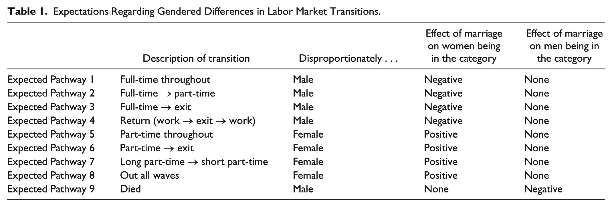
Based on this reasoning, Expected Pathways 1 to 3 are assumed to be dominated by men because they all start with working full-time in the earlier stages, whether they involve being full-time throughout (Expected Pathway 1), moving from full-time to part-time work (Expected Pathway 2), or moving from full-time work to complete exit (Expected Pathway 3). We expect movements into part-time work to be less common than the more traditional “male breadwinner pathways” of working full-time throughout or retiring/exiting from full-time work. In addition, it is suggested that returning to work after an absence is likely to be disproportionately a “male” transition, because women will be less likely than men to return to work for financial reasons, given the importance of gender norms/resources (Expected Pathway 4).
In the case of each of these four expected “male” pathways, we suggest that a “modified male-breadwinner” logic means that marriage reduces the likelihood of women being in these “male” transition types. This is because the (modified) male breadwinner logic assumes that there is a male breadwinner. In the case of single women, there would be no “male breadwinner” to influence employment patterns. The influence of marriage on employment for men, on the contrary, is not predicted to be large. This is because men are more often than not the “breadwinner” when they live in couples, and by definition, they are the “breadwinner” when they are single as well. The only impact marriage is predicted to have on men is that it will reduce the likelihood of dying in “early older age,” because marriage is known to have positive health benefits for men (Grundy & Tomassini, 2010; Expected Pathway 9).
The remainder of the trajectory types predicted in Table 1 is expected to be dominated by women. The first two are fairly traditional: working part-time throughout the period and moving from part-time work to exit (Expected Pathways 5 and 6). In addition, we allow for the possibility that women may also downsize, from long to short part-time hours (Expected Pathway 7). Finally, we predict that women are more likely than men to be out of work throughout the entire period, consistent with a “pure” breadwinner logic (Expected Pathway 8). Overall, we predict that being married will increase the likelihood of women being in these typically “female” clusters. If there is no male partner, women may need to work more hours for financial reasons and they may have less caregiving tasks enabling longer working hours. Once again, we expect marital status to have no large impact on men being in these female-dominated clusters, because men are similarly likely to be the “main breadwinner” within households, irrespective of whether they are married or not.
Analytical Strategy
Introducing the Strategy
As discussed above, we want to ascertain first whether “employment pathways” emerge from the data that can be categorized as being dominated by men or women, consistent with the “modified male breadwinner” logic (Research Question 1). In doing so, we need to use sophisticated analytical techniques to categorize potentially complex transitions over an extended period of time (10 years) into trajectory types. This is important because we want to take into consideration the ordering of events, and whether, as a result, we can identify structured pathways, such as individuals moving from full-time to part-time work in older age. In this example, we might expect to see a cluster of people moving from full-time employment, to part-time work, to retirement, but the exact timing of events is of less importance than the ordering. We therefore use sequence and cluster analyses to allocate people to different pathway-cluster types.
Sequence analysis has been little used in relation to older worker trajectories, and previous studies have not used it in exactly the same way as it is used here. Riekhoff (2016), for example, measures de-standardisation and differentiation of work/retirement transitions in the Netherlands, rather than clustering pathways into different “types.” Fasang (2010), alternatively, looked at work/retirement trajectories in the United Kingdom and Germany in the period up to 2006. Although Fasang’s (2010) study found that part-time employment was more common among women than men in both countries, it is difficult to ascertain from the analysis exactly how common these pathways were for women, as this was not the main focus of the article. Furthermore, our study differs from Fasang (2010) because we explicitly examine the influence of marriage on the working-time pathways women and men follow. This is important because it is a true test of whether the “modified male breadwinner” model of O’Connor et al. (1999) influences female employment as hypothesized. Finally, Fasang’s (2010) study focuses on a cohort that was born between 1923 and 1940, up to almost 20 years earlier than the one examined here. It is therefore possible that gender norms have changed for the more recent cohort examined here, born during/after the Second World War (between 1942 and 1952).
To identify whether or not pathways are dominated by women or men, the results are presented as predicted likelihood of women and men being in each pathway cluster, based on multinomial logistic regression analyses. Following this, separate multinomial logistic regression analyses are presented for women and men, to examine the extent to which marriage influences women being in typically “male” or “female” clusters, as per Research Question 2. Before we can outline these approaches in more depth, it is important to examine the data used and the variables constructed.
Data
This article analyzes the first six waves of ELSA (Marmot et al., 2015). 1 We look at individuals who were in the first wave of the ELSA survey (2002/2003) aged 50-60 and follow them for 10 years (until 2012/13). By selecting people aged between 50 and 60 (inclusive) in the first wave, and 60 to 70 in the final wave, we therefore exclude older individuals for whom work/retirement transitions over the period are less likely. These people were born between 1942 and 1952 and reach(ed) the state pension age between 2002 and 2014 (women) or 2007 and 2017 (men). 2
We selected individuals aged 50 to 60 in Wave 1 of the survey. Less reliable “proxy interviews” answered by someone else were then deleted. Some individuals had been added to the survey at later waves, so we selected only individuals participating in all six waves to be able to track their trajectories. Finally, we selected only individuals who were core members of the dataset as these were the respondents aimed to be representative for the population. This resulted in 14,742 observations. Aside from missing data due to wave nonresponse (included under Step 3 above), there is a smaller amount of item-missing data as not all respondents answered all questions used in this article. Because of item-missing data at any single wave, we ended up with 13,716 observations (93.04% of remaining sample) nested in 2,286 respondents. In Web Appendix A, there is a deeper consideration of the wave-missing and item-missing data. 3 In general, individuals with a higher educational level and a higher income level were less likely to having missing waves. Individuals who were married were more likely to have at least one missing wave, but there was not a significant gender, age, or health difference.
Variables for Sequence Analysis
In sequence analysis, the variable of interest is the sequence (or pathway) itself. A sequence consists of various states that individuals can be in that are mutually exclusive. In each wave, an individual can be in one state at the time, and the pathway shows the trajectory of the individual. The states we looked at were whether someone was in paid employment (full-time or part-time), in self-employment (full-time or part-time), not employed, or dead. We included people who died over the period to avoid biasing the estimates because this is a form of attrition that is likely to vary by gender, age, education, and health. Individuals who died over the observation period were given the state “dead” for that wave and all subsequent waves. Hence, to give an example, an individual’s sequence can be full-time employed in the first two waves, part-time in the subsequent three waves, and dead in the last wave.
We now describe how each state is exactly measured. The employment status of individuals was taken from a derived variable in the dataset which indicated whether the respondent was employed or self-employed. People who were not in paid work or self-employment were considered not-employed. Individuals in paid employment and self-employment were categorized by how many hours they usually worked in a week. We divided this variable in three categories: (a) short part-time work (1-15 hr/week), (b) long part-time work (16-34 hr/week), and (c) full-time (35 hr/week or more). We make a distinction between different types of part-time work because we want to allow for the fact that a “female” downsizing in employment may occur, from “large” part-time to “small” part-time (Expected Pathway 7). We follow many previous U.K.-based studies by using the cutoff of below 16 hr a week for “small” part-time work (see, for example, Harkness & Evans, 2011; Kodz et al., 2003). 4 There is no official definition of how many hours full-time work equates to, but we followed U.K. government statement that “a full-time worker will usually work 35 hours or more a week” (Government Digital Service, 2016). Individuals were categorized separately as employees or self-employed because we expect self-employed individuals to find it easier to reduce their working time (Lain, 2016); on the basis of previous research, we do not expect many older employees to move into self-employment in older age (Parker & Rougier, 2007).
Other Variables
In addition to the labor market variables described above, several variables were used to predict which pathway clusters people ended up in. First, we looked at marital status in the first wave, drawing on the survey question: “What is your current legal marital status?” When the respondent was currently married (regardless of whether this was a first marriage or not), the respondent was considered married. The respondent was considered “not married” if they were never married, legally separated, divorced, or widowed. As more than 70% were currently married, we made no further distinction.
It is important to take into account a range of other factors, beyond marital status, that are likely to influence the employment of older married and unmarried women and men. This includes age differences, because the likelihood of working decreases as people get older (Lain & Vickerstaff, 2015), and there may be differences in the average age of married and unmarried individuals. Likewise, education is known to increase the likelihood of working in older age (Lain & Vickerstaff, 2015), and in this cohort, older men are (marginally) more likely to have tertiary education than women (Organisation for Economic Co-operation and Development [OECD], 2012). In addition, health influences the ability to work, and married men are likely to have better health than their single counterparts; the evidence for women is less conclusive (see Grundy & Tomassini, 2010; Robards, Evandrou, Falkingham, & Vlachantoni, 2012). Finally, we might expect the financial need to work to vary between different groups—for example, we might expect this to be stronger for single women than men (Tinios, Bettio, & Betti, 2015). In the analysis that follows, we therefore “control” for differences in age, education, health, and income.
We distinguished between the age groups 50 to 53, 54 to 56, and 57 to 60 at the first wave. We did not use age as a continuous variable, because it was not normally distributed. Each age group contained approximately a third of the respondents.
We looked at someone’s educational level in the first wave, recoding the existing variable in the dataset into one distinguishing between “high,” “medium,” and “low” qualifications. “High education” included “NVQ4 / NVQ5 / Degree or equivalent” or “higher education below degree.” “Medium education” included “NVQ3 / GCE A Level equivalent,” “NVQ2 / GCE O Level equivalent,” or “NVQ1 / CSE other grade equivalent.” Finally, “low education” constituted having “no qualification” or having a “foreign / other” qualification. The inclusion of “foreign / other” qualifications under “low education” is consistent with previous research using this dataset (see, for example, Lain, 2011).
Income was defined as the equivalized version of the total benefit income of a unit. This measure was adjusted for unit size (variable name in dataset: eqtotinc_bu_s). This measure looks at income from employment, self-employment, state benefits, state pensions, private pensions, assets, and other sources. Because this variable was not normally distributed, we considered in which quartile of the distribution individuals fell.
Finally, we looked at whether the respondent had any long-standing illness or disability in the first wave and whether this affected the respondent’s activities in any way. This lead to three categories: (a) no illness or disability, (b) has illness or disability that does not limit activities, and (c) had illness or disability that does limit activities. Descriptive statistics of all variables can be found in Table 2.
Descriptives Table.

Source. English Longitudinal Study of Ageing (ELSA) Waves 1 to 6.
Note. Complete data, separate descriptive statistics for women and men. All variables are dichotomous variables.
Method
Sequence analysis
Sequence analysis is becoming more popular among social scientists as it is perceived to be more directly related to studying the trajectories that individuals’ follow, which is of particular interest in life course research. As Aisenbrey and Fasang (2010) claim, “Sequence analysis is a tool that can reduce the imbalance between the core concepts of transition and trajectory in life course research; sequence analysis can bring the trajectory, the actual ‘course,’ back into research on the life course” (p. 421). It is mostly a descriptive and exploratory technique that hopes to unveil patterns or structure in the data (Elzinga, 2003).
To assess how similar sequences are, we make use of the concept of subsequences. A subsequence is a part of the total sequence that occurs in the same order as the total sequence when reading from left to right (Elzinga, 2007). Note that reading from left to right, one state precedes another state, but that these states do not have to follow each other directly (Elzinga, 2003). Because of the focus on subsequences, it places special attention to the order in which states occur. This may be important, for example, because there is a qualitative difference between someone first reducing their working hours and then quitting work all together, and someone moving from full-time work to inactivity, followed by part-time work.
As a measure of variation between sequences, we look at the longest common subsequence (LCS, Elzinga, 2007). The LCS compares the subsequences between sequences and chooses the longest subsequence that sequences have in common. The longer the subsequence, the more similar the sequences are. Rather than comparing each possible subsequence (a demanding process given that a sequence of length n has 2 n subsequences), it uses a dynamic algorithm to calculate the LCS (see Elzinga, 2007, for more details). This measure has previously been applied to a variety of topics, such as de-standardization and similarity of family formation (Elzinga, 2007) and job searching and job finding behavior of people who are released out of prison (Sugie, 2014). As a robustness check, we also looked at the Hamming Distance and the Dynamic Hamming Distance (see Web Appendix D), but clusters remained largely the same and did not affect the main conclusions provided in this article.
Cluster analysis
Following most previous research, we use cluster analysis after the sequence analysis, in our case to identify different late career pathway clusters. Cluster analysis aims to summarize the sequence similarity measures in a small number of trajectory types (e.g., Abbott & Hrycak, 1990; Biemann & Datta, 2014; Brzinsky-Fay, 2007; Elzinga, 2003; Fasang, 2009; Wahrendorf, 2014). Choices have to be made as to which cluster algorithm to use and how to decide on the optimal number of clusters (Aisenbrey & Fasang, 2010). We used partitioning around medoids clustering (PAM-clustering; Kaufman & Rousseeuw, 1990), which is considered a more robust version of k-means clustering (Partitioning Around Medoids, n.d.). For an example of the use of PAM-clustering, see Borghetto (2014).
To decide on the number of clusters, we look at silhouette width and at the ratio of within/between variance of the cluster solutions. We combine information from these two sources with looking at the substantive meaning of each cluster (based on our hypotheses) to decide on a final cluster solution. The basic idea of the silhouette width s(i) is that for each sequence in the data it is investigated whether it fits better in its own cluster or in a neighboring cluster. The closer the number s(i) is to 1, the better the fit with the own cluster in comparison with the next closest cluster. The closer to −1, the more the opposite applies. When the value is zero, the observation is just as likely to be in its own cluster as in the neighboring cluster (Reynolds, Richards, De la Iglesia, & Rayward-Smith, 2006). Kaufmann and Rousseeuw (1990) state that if a silhouette has an average width of 0.5, then there is a reasonable classification achieved. If there is only a small silhouette width (say below 0.2), then there is no real cluster structure (Everitt, Landau, Leese, & Stahl, 2011). This method on how to decide on the number of clusters has also been included in, for example, Borghetto (2014) and Fasang and Raab (2014).
Looking at the within and between variance of the cluster solution has been discussed in several sequence analysis papers (e.g., Abbott & Hrycak, 1990; Aisenbrey & Fasang, 2007; Aisenbrey & Fasang, 2010). Aisenbrey and Fasang (2007) suggest as a rule of thumb that the “mean within cluster distance should not be higher than half of mean between cluster distances, in order to indicate a valid identification of distinct sequence patterns” (p. 25). We follow this rule in this article.
Multinomial logistic regression analysis
To answer the two research questions, multinomial logistic regression analyses were conducted using the clustered pathways identified in the previous stages. First, regression analysis was conducted on the sample of women and men together; from this, the overall margins of women and men being in each cluster were calculated (cf. Stata Margins Manual). These show the adjusted (predicted) probability of women and men being a particular cluster while controlling for background variables (marital status, income, education, health, and age). From this, we are able to answer Research Question 1, namely, whether or not there were differences between women and men in the predicted likelihood of being in a particular cluster (after controlling for other factors). Following this, multinomial logistic regressions were run separately for women and men, enabling us to see whether or not marriage influenced the employment of women as predicted (Research Question 2). For both questions, the adjusted (predicted) probabilities were calculated using average marginal effects (AMEs). This means that, rather than keeping the control variable constant at their average, the adjusted (predicted) probabilities were averaged using the observed values of the control variables (for more detail, see Williams, 2012). Do note that these are average marginal effects and we do not predict the same increase or decrease in likelihood for all women and men.
The data manipulation, sequence analysis, and cluster analysis were conducted in R (version 3.2.0, R Core Team, 2015), with add-on packages used as required, 5 and the multinomial logistic regression was performed using Stata 12.1. Several sensitivity checks are presented in Web Appendix D. These include the impacts of weighting the analysis, using a different type of clustering (Ward clustering), using a different seed (to see the role of the random component of PAM-clustering), and using a different full-time working hours cutoff (of 30 hr/week). Although there were some differences in clusters found with the different specifications, in general, the main conclusions of this article stand.
Results: Which Clusters
Before turning to our research questions, we first present the results of our sequence and cluster analyses. We used the LCS to calculate the difference between sequences, followed by a cluster analysis. We investigated cluster solutions ranging from two to 30 clusters (see Web Appendix E). The lowest number of clusters that fitted our criteria (within/between variance ratio below 0.50 and average silhouette width of 0.50) was the five-cluster solution. These clusters were, however, fairly broad and not informative. The 11-cluster solution was interpretable given the expected pathways listed in Table 1, and broadly met the requirements of having a within/between variance of below 0.50 (specifically, 0.22) and an average silhouette width close to 0.50 (specifically, 0.48). Figure 1 gives a visual representation of our clusters. The Sequence Index Plots show all sequences that are found in the cluster. Each line represents one sequence (i.e., the observed pathway of one individual). The State Distribution Plots show at each wave all the states that are found in each cluster. Both are used to interpret the clusters we have found.
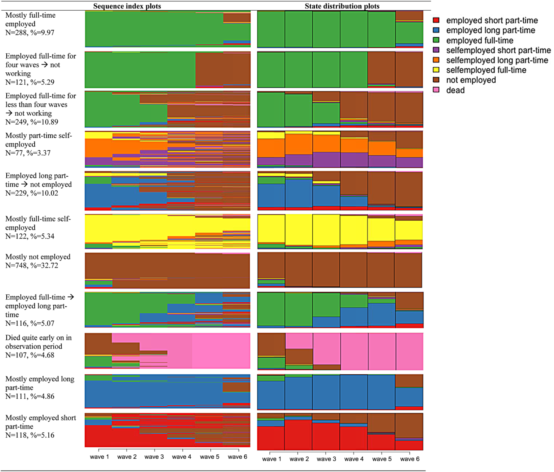
Distribution plots.
We decided to merge the clusters “employed full-time for four waves → not working” (row 2 in Figure 1) and “employed full-time for less than four waves → not working” (row 3 in Figure 1) because we were not theoretically interested in whether someone was employed full-time for exactly four waves. There are two reasons for this. First, the transition is the same (moving from being employed full-time to not working). Second, due to age differences between respondents, there is nothing specific about being employed full-time for exactly four waves. Hence, we do not perceive these two clusters as meaningfully different. This leaves us with a total of 10 clusters.
Results: “Male” and “Female” Clusters? (Research Question 1)
Figure 2 shows the 10 remaining clusters with the adjusted (predicted) probabilities of women and men being in each cluster to give an idea about whether there are indeed “male” and “female” clusters. These predicted probabilities are based on a multinomial model with men and women in the same model (for further detail, please see the “Analytical Strategy” section). The expected pathway to which each cluster relates is given in brackets (e.g., EP1 = Expected Pathway 1).
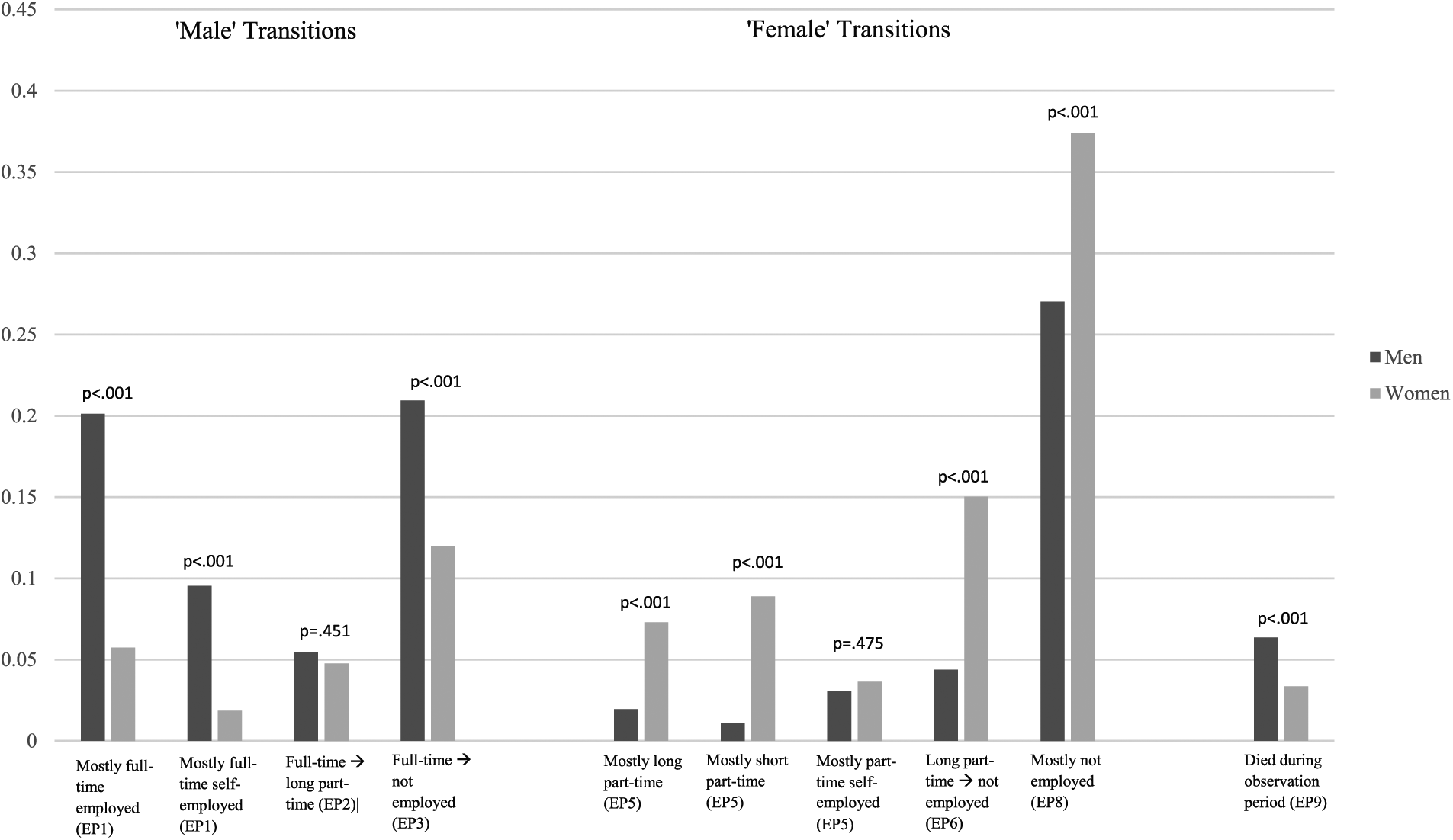
Overall likelihood of being in each cluster.
The first thing to note is that, contrary to the arguments of Cridland (2016) and others, there is no strong evidence of people moving from full-time to part-time work. The adjusted probability of being in the category “full-time → long part-time” was only around .05. Likewise, no cluster emerged that represented movement from long part-time to short part-time work (Expected Pathway 7). In addition, no clusters emerged relating to individuals returning to work following exit (Expected Pathway 4), suggesting that this is very rare pathway for people to take (see also Kanabar, 2012). Instead, all but one of the pathway clusters involved doing the same activity for at least “most” of the period, or moving from one activity to exit. The pathways people took were also strongly gendered, consistent with modified male breadwinner norms discussed above.
Starting with the typically “male” transitions on the left of the figure, for men the most likely pathway clusters were “mostly working full-time” over the period, or moving from full-time work to complete exit. A significant minority of men were also working “mostly full-time self-employed” throughout. Women were significantly less likely to be in each of these three pathway clusters, supporting Expectations 1 and 3. There was no significant difference between women and men in terms of being in the “full-time → long part-time” cluster (lending little support to Expectation 2); this reflects the fact that both women and men had a low predicted likelihood of “downsizing” into part-time work.
Moving onto typically “female” transitions, women were significantly more likely to be in four out the five of the clusters identified (supporting Expectations 5, 6, and 8). The one exception was “mostly part-time self-employed,” presumably because the female tendency to work part-time was counterbalanced by the higher likelihood of men being self-employed. Again, both men and women were quite unlikely to be in this cluster. Women with work histories during the period were most likely to move from “long part-time work → not employed.” Finally, women had a significantly higher adjusted (predicted) probability than men of being in the category “mostly not employed” over the period, consistent with a “pure” breadwinner logic. Men were significantly more likely to die over the observation period (Expectation 9), consistent with what is known about women having longer life expectancies on average (ONS, 2016).
Results: The Importance of Marriage for Employment of Women (Research Question 2)
To summarize the above analysis, the adjusted probabilities of being in different clusters suggest that there are strong gender differences in employment. However, to examine whether this is consistent with a male breadwinner model, we need to investigate the extent to which marriage relates to female employment pathways. Table 3 presents the results of the multinomial logistic regression analysis of women only. The “overall” results at the top of the table show the overall margins of women being in each cluster; these are similar to those shown in Figure 2, the results only differing slightly because they are not affected by having men in the regression. Below this, discrete differences indicate how being in one category (e.g., “married”) changes the likelihood of being in a particular cluster (e.g. “mostly full-time employed”), relative to a reference category (in this case “not married”). A discrete difference of −0.06, for example, shows that married women were on average six percentage points less likely to be “mostly full-time employed” than their unmarried counterparts; the fact that this result is in bold indicates that the difference is statistically significant at p < .05.
Average Margins/Average Marginal Effects of Being in a Cluster Solution: Women Only.

Source. English Longitudinal Study of Ageing (ELSA) Waves 1 to 6.
Note. dd stands for discrete difference, p for significance. The “Overall” row shows the overall margins. This differs from Figure 2 because the average is now based on women only. All other variables show the discrete difference based on average marginal effects. The significance of the variable is calculated with a likelihood ratio test. The significance of the variable per cluster with margins. Variables that are significant with p < .05 are shown in bold. EP = expected pathway.
Taken as a whole, the results show that marital status was strongly associated with the employment paths women followed, consistent with a modified male breadwinner logic. We predicted above that being married would reduce the likelihood of women being in “male” pathway clusters, and increase the likelihood of them being in female clusters. For the most part, this proved to be true. Being married was related to a significantly lower average likelihood of women being in the “male” clusters “mostly full-time employed,” “full-time → long part-time,” and “full-time → not employed” (providing support for Expectations 1, 2 and 3). There was no significant difference between married and unmarried women in the category “mostly full-time self-employed,” but as we saw in Figure 2, there were very few women predicted to be in this category in the first place. For the “female” transitions, being married was related to a higher average likelihood of being in three out of the five clusters: “mostly short part-time,” “long part-time → not employed,” and “mostly not employed” (providing some support for Expectations 5, 6, and 8). This meant that there was no significant difference between married and unmarried women in relation to “mostly part-time self-employed,” although once again this was a small category (see Figure 2).
Contradicting our expectation, there was no significant difference between married and unmarried women in relation to being “mostly long part-time.” The other results show that low incomes were related to a higher likelihood of being “mostly not employed.” presumably because it signifies disadvantage, as did poor health and being older. For women, being married had no significant effect on dying in the period.
Moving onto the results for men, we predicted that marital status would not have a large impact on the propensity to be in “male-dominated” or “female-dominated” clusters. This was because in most cases men would be the “breadwinner,” irrespective of whether they were married or not. For the most part, this proved to be the case. The only significant difference in this regard was that the average adjusted (predicted) probability to be in the category “full-time → long part-time” was significantly higher for married than unmarried men. It should be noted that this was a relatively small category for men (see Figure 2). Nevertheless, it is an interesting finding. One possible explanation is that an admittedly small number of women and men equalize their working hours to some degree in older age, with married men reducing their hours and married women continuing to work long part-time. To some degree, this may reflect the desire for men to remain in work on an at least equal capacity to their partners, if their partners are “too young” to retire. If so, this would reflect a reluctance to completely reject male breadwinner norms by retiring before their partner. Alternatively/additionally, it may be the case that men without a partner at home see less reason to reduce their hours, something for future research to examine. The other results in Table 4 are broadly similar to that of women in relation to the impact of age, health, and income on employment. The only exception to this is that married men had a reduced likelihood of dying during the period, something that was not significant for married women.
Average Margins/Average Marginal Effects of Being in a Cluster Solution: Men Only.

Source. English Longitudinal Study of Ageing (ELSA) Waves 1 to 6.
Note. dd stands for discrete difference, p for significance. The “Overall” row shows the overall margins. This differs from Figure 2 because the average is now based on men only. All other variables show the discrete difference based on average marginal effects. The significance of the variable is calculated with a likelihood ratio test. The significance of the variable per cluster with margins. Variables that are significant with p < .05 are shown in bold. EP = expected pathway.
Discussion
It is often claimed that more “gradual” paths to retirement have emerged, including moves from full-time to part-time work, and that this will facilitate an extension of working lives. In this context, it is noted that part-time rates of older workers are comparatively high. This article starts from the proposition that, rather than representing movements into part-time work, many women are already in part-time work when they enter older age. We draw on O’Connor et al. (1999) to argue that the United Kingdom represents a “modified male breadwinner” system, in which married women often work part-time during their career to supplement the incomes of their typically full-time working partners. This, it is suggested, perpetuates the continuation of part-time work among women and full-time work among men. In such a system, there is a strong “gender asymmetry,” which means that female employment in older age is likely to be concentrated in typically “female” employment pathways, such as working part-time throughout or retiring/exiting employment from part-time work. At the same time, in the absence of a “male breadwinner,” unmarried women may be more likely than their married counterparts to be in male-dominated full-time employment pathways. For men, it is suggested that marriage is less important in whether they are in male-dominated or female-dominated employment pathways. This is because men are likely to be the “breadwinner” irrespective of whether or not they are married. To investigate this, we examined the employment pathways people followed over a 10-year period from age 50 to 60 till 60 to 70, using ELSA. We used sequence/cluster analysis to identify different types of employment pathway clusters that people followed over the period. We then used multinomial logistic regression to calculate the likelihood of women and men being in each cluster (controlling for other factors), to see whether gender was important in distinguishing between the clusters. Finally, we ran separate multinomial logistic regression models for women and men to see whether marriage mattered for whether women ended up in female-dominated employment pathway clusters.
Despite contemporary debates about work and retirement, we found little evidence of individuals downsizing from full-time to part-time work. The pathways taken were, as predicted, highly gendered, and broadly consistent with the modified male breadwinner model of O’Connor et al. (1999). Men working during the period were most likely to work full-time throughout, or move from full-time work to retirement/exit. Women working over the period were more likely to work part-time throughout, or to move from part-time work to retirement/exit. Women were also significantly more likely to be “mostly not employed” during the period. Consistent with a breadwinner model, the results also indicated that being married was associated with a significant increased likelihood of women being in “female-dominated” pathway clusters, and a reduced likelihood of being in male-dominated pathway clusters. For men, on the contrary, marriage was only associated with reducing the likelihood of dying, or moving from full-time work to part-time work. However, in the latter case, relatively few men (or women) move from full-time work to part-time employment, reducing the importance of this.
In terms of limitations, it should be noted that as with any survey-based analysis, nonresponse and missing data were not randomly distributed. As missing data were more common among those with low education and incomes, there may be biases toward the pathways of less disadvantaged individuals. However, as discussed above and in the web appendix, we conducted a range of robustness checks that strongly suggest that the main conclusions of the article stand. It should be noted that with these analyses, we obviously cannot definitively prove the casual influence of marriage on employment patterns of women and men, although the evidence is arguably consistent with such an interpretation. Finally, these types of sequence analyses do not allow for a dynamic study of influences on pathways and we could therefore not investigate how changes in marital status were related to changes in employment. Future research may want to assess this further.
Conclusions for policy and future research
The results have negative implications for attempts to extend working lives among older women. If a modified male breadwinner model continues to dominate the divisions of paid and unpaid labor in the household, women will stay in part-time work, which may often be unstimulating and badly paid. Qualitative evidence suggests that women may not want to continue working in marginal and boring part-time jobs, and so will exit when they have an opportunity to do so (Loretto & Vickerstaff, 2013). In part, this could be a cohort effect, as more recent cohorts of women have made inroads into more senior occupations to some degree and the gender pay gap has been reduced for younger women (although it is a long way from being eliminated). That said, although women are returning to work after childbearing more quickly than their mothers (Dex, Ward, & Joshi, 2008), part-time work remains stubbornly high at around 40%; this suggests that women could continue to follow their husbands in the terms of the work/retirement decisions that they make. These findings are therefore likely to continue to have some relevance for future generations, although it is important for future research to monitor the extent to which this is changing using longitudinal data on different cohorts. In this regard, it will be interesting to see whether male and female employment patterns become more similar with the equalization of state pension ages.
In sum, the analyses in this article show that O’Connor et al.’s (1999) model of the “modified male breadwinner” still has resonance for older women (and men) in England today. This article makes a contribution by theorizing what late career employment transitions will “look like” for married and single women and men living in a “modified male breadwinner” country. It is for future research to extend the theoretical and empirical analyses by comparing employment transitions in England with those in the United States, where late career transitions of men and women are likely to be relatively similar (Lain & Vickerstaff, 2015) given the policy focus on “gender sameness” (O’Connor et al., 1999).
To conclude, this article has shown that women and men differ in their later employment patterns and that these gender differences appear to be related to traditional gender roles. Although changes in state pension ages may nudge people into continuing to work for a little longer, the evidence presented here suggests that people are currently not, for the most part, downshifting in terms of the number of hours they work. There was, perhaps surprisingly, little evidence that gradual retirement has become the norm for women and men, notwithstanding the wealth of evidence that the idea of gradual or phased retirement through flexible working is popular (Loretto & Vickerstaff, 2015; Maitland, 2010; Smeaton, Vegeris, & Sahin Dikmen, 2009). At least for this cohort, it seems a long way off to suggest that people are moving into “bridge employment” as a means of working longer, as is now assumed to be the case in the United States. In any eventuality, to downsize in employment, people need jobs worthy of downsizing in. Therefore, if we want to encourage older women to work longer, we need to support them in having fulfilling careers on equal terms to men long before they reach older age.
Footnotes
Acknowledgements
The authors thank Chris Phillipson and participants of the Centre for Longitudinal Studies Cohort Studies Research Conference 2015 and the European Sociological Association (ESA) PhD Workshop “Long Live the Active!? A Critical Review of Active Ageing” (2015) for their valuable comments on earlier versions.
Declaration of Conflicting Interests
The author(s) declared no potential conflicts of interest with respect to the research, authorship, and/or publication of this article.
Funding
The author(s) disclosed receipt of the following financial support for the research, authorship, and/or publication of this article: This article is funded through the “Uncertain Futures: Managing Late Career Transitions and Extended Working Life” project by the Economic and Social Research Council (ESRC), ESRC reference: ES/L002949/1.
Notes
Author Biographies
![]() for details.
for details.
![]() for details.
for details.