Sage Journals: Discover world-class research

Abstract

Theoretical and empirical studies have focused on discretionary investments such as research and development (R&D) and advertisement as value-creating activities. This empirical research article examines the determinants of the discretionary investment policy of food sector firms in India. The study aims to analyze the impact of financial policies and firm characteristics on the discretionary investment strategy of the food industry firms. The article uses the partial least squares structural equation modeling (PLS-SEM) to understand the drivers of discretionary investment policy of food sector firms. The study finds that investment policy of firms is a major determinant of profitability of food sector firms. Higher investments in capital expenditures and working capital result in higher profitability. Management efficiency significantly influences firm profitability. The results suggest that riskier firms in food sector might focus on R&D investments as a strategy to generate more cash flows. Size of firm is negatively related to R&D intensity. Smaller firms in food sector tend to invest more in R&D. The study does not provide evidence to suggest that profitable firms invest more in R&D activities.

Keywords

general management management social sciences manufacturing operations management industrial and organizational psychology organizational behavior strategic management organizational theory and business policy multi-variate analysis research methods discretionary investments partial least squares path analysis food industry

Introduction

Firms undertake innovation to create value for stakeholders. Sustainable process-driven innovation transforms ideas into vital intellectual property which leads to shareholder value creation through increased revenues. Contemporary strategic thinking posits that firms can gain competitive advantage by increasing its research and development (R&D) and advertising expenditures. R&D-based strategies attempt to generate knowledge assets which enable firms to develop either superior products or more efficient production techniques. Advertising seeks to differentiate the firm’s product from those of competitors. Many research studies have provided evidence that advertising and R&D expenditures have large positive and consistent influences on the market value of the firm. These studies suggest that advertising and R&D have statistically significant and quantitatively important impact on profit rates which provide a measure of market performance. Despite the postulated importance of these expenditures, firms still consider these expenditures as discretionary. During difficult times, firms often reduce discretionary investment expenditures due to reduction in income. The discretionary investment policy of firms can be viewed as strategic in nature. The present study aims to analyze the determinants of discretionary investment behavior of firms in food sector. Indian food products industry is chosen for this study due to its complexity and diversity. Food and food products are the biggest consumption category in India, with spending on food accounting for nearly 21% of India’s gross domestic product (GDP) and with a market size of US$181 billion.

Review of Literature

Studies of Drucker (1986), Jacobs (1991), and Porter (1992) suggested that firms compromise on discretionary investments during difficult economic times. However, studies such as Srinivasan, Gary, and Arvind (2005); Clark (2008); Kamber (2002); and Graham and Kristina (2008) viewed that there are advantages of increasing these activities when other firms are compromising it. When other firms are reducing these activities, an emptiness is created in the market, which provides opportunity to differentiate and gain market through advertisement. Nishimura, Takanobu, and Kozo (2005) pointed that firms which compromise on R&D often deviate from their long-term growth path and would significantly harm the company in long run.

Literature on R&D and advertisement decision has come a long way since structure, conduct and performance (SCP) approach was proposed by Mason (1939) and Bain (1951). These studies suggested that differences in conduct with respect to R&D and advertisement behavior can be linked to structure of the industry. Highly concentrated industry behaves differently compared with less concentrated industry. The SCP approach initially focused on inter-industry differences. The focus then shifted to intra-industry differences. Studies like that of Wernerfelt (1984) and Barney (1991) postulated that the differences in firm performance are due to unique firm-specific factors or resources. These specific resources are valuable, rare, inimitable, and non-substitutable. Marketing and innovations facilitate firms to develop these specific resources for gaining competitive advantage in long run.

During the 1960s, management theory and research began to adopt a new orientation which represented a middle ground by improving the generalizability of the former, while obtaining richer characterizations than the latter (Valarie, Rajan, & Carl, 1988). The contingency approach in strategy literature advocates that different strategies are contingent on competitive settings of businesses. Competitive settings are defined in terms of environmental and organizational contingencies. These contingencies interact with firm-level factors, which ultimately affects the strategies firms choose.

George and Agnes Cheng (1992) found that the differences in strategies are due to type of offering and market type. Studies of Schumpeter (1961), Arvanitis (1997), and Cohen, Levin, and Mowery (1987) found that the size of the firm is an important variable that determines R&D decision. Lee and Sung (2005) found that the relationship between R&D and size is probably stronger for industries with greater technological opportunities. Studies by Guariglia (2008) and Hovakimian (2009) suggested that relationship between R&D and size is positive for firms with higher capital intensity.

Ryan and Wiggins (2002) pointed that firms with high growth opportunities have more incentives to invest in R&D once a considerable percentage of their value is sourced from assets which are not in place. Del and Papagni (2003) on the basis of summarized studies of 20 years suggested that the relationship between growth of the firm and research intensity could not be established by many studies. The free cash flow hypothesis advanced by Jensen (1986) stated that managers endowed with free cash flow will invest it in negative net present value (NPV) projects rather than pay it out to the shareholders. Henry and John (2000) suggested that expected returns and cash flows are important explanatory variables of R&D intensities.

Generally Indian firms prefer technology purchase route by paying royalty. This helps the firms to reduce uncertainty surrounding R&D investments. Katrak (1989) found that imported technology helped in promoting R&D activities in Indian firms. Siddharthan (1992) found the relationship between imports and R&D to be complementary. However, R&D intensive firms often see outsourcing as an impediment, especially during 1990s. Michael (2005) found that post nineties, R&D intensive industries have increasingly entering into partnership relationship with outside suppliers.

Myers (1977) suggested that financial leverage often influence firm’s strategies through agency problem with its shareholders. Ho, Mira, and Chee (2006); Long and Ileen (1983); Grullon and George (2006) found that financial leverage is negatively related to both R&D and advertising spending. Jensen and William (1976) and Raji, Gary, and Shrihari (2011) suggested that higher level of debt in the capital structure moderates the effects of R&D and advertisement in influencing the profitability during difficult times. Kotabe (1990) confirmed that profits have a positive relationship with R&D initiatives. Paunov (2012) found that small companies in times of economic crisis faces difficulties in keeping their level of R&D investment. As debt increases, the expected costs of financial distress also increase. Cost of financial distress is called the underinvestment problem. Direct expenses associated with administration of the bankruptcy costs appear to be small. Indirect costs are huge, and the most important indirect costs are likely to be reductions in firm value that result from cutbacks in promising investment when companies get into financial difficulty. Managers may cut back or postpone major capital projects, R&D, and advertising.

The study by Hirsch and Gschwandtner (2013) revealed that the degree of profit persistence in the food industry is lower compared with other manufacturing sectors due to strong competition among food processors and high retailer concentration. Furthermore, firm size is an important driver of persistence, whereas firm age, risk, and R&D intensity have a negative influence. The paper by Hirsch and Hartmann (2014) used autoregressive models and Arellano–Bond dynamic panel estimation to suggest that cooperatives which account for around 20% of all firms in the European diary processing sector are not primarily profit oriented. The panel model reveals that short as well as long-run profit persistence is influenced by firm and industry characteristics.

Theoretical Postulates

R&D has become a key strategic driver to improve the products and services in the modern world based on new technology innovation. This article provides evidence on the relationship between the financial policies of firms in the food industry and R&D activities. The study explores whether firms with significantly larger financial performance have an intensive investment strategy in R&D.

R&D investment strategy is long-term oriented and signifies uncertainty. New products and services are very critical for competitive success. It may be noted that managers are risk averse and may avoid R&D investments for the following reasons. Intangible investments have a greater probability of failure than tangible investments. R&D being a long-term growth investment involves technological and competitive risks. The returns from intangible investments like R&D are more remote in time compared with returns from tangible investments. An important characteristic of R&D expenditure is irreversibility in which if a firm decides to stop a R&D project, it will not be able to recover all the money invested, the reason being that these investments are partly specific to the firm and cannot be sold at their acquisition costs. The spillovers relating to processes of specific R&D will make it possible for competitor firms to gain competitiveness at a lower cost on account of the imitation of the processes.

In the context of risky nature of R&D investments, it can be hypothesized that firms with greater financial performance involve in active R&D investment strategy. Thus, R&D investment strategy is a function of the financial performance and other financial policies of the firm. It can be stated that R&D investment strategy of food sector firms are a function of profitability, size, liquidity, leverage, cash flow, and other external characteristics.

Value drivers are crucial for value maximization. Value drivers can be classified into operational, investment, and financial. Firms with higher growth rate in sales, assets, and profits tend to have higher profits. Higher investments in form of capital investments and working capital result in higher profitability. Improvement in management efficiency or operational efficiency would lead to higher value for firms in the form of increased profitability. Higher profitability acts as an incentive for firms to undertake more intensive discretionary investments like R&D activities. Higher profits will lead to higher R&D intensity. R&D investment intensity is also a function of the firm’s size, liquidity, leverage, cash flow, and risk characteristics. Large firms tend to make more R&D investments. Firms with higher leverage tend to make lower R&D investments. Firms with high liquidity and cash flows tend to invest more in R&D activities.

The study assumes that the discretionary investment policy of food sector firms in the form of R&D expenses and advertising expenses is a function of critical financial characteristics of the firm such as size, growth, financial leverage, risk characteristics, investment decision policy, asset utilization efficiency, cash flow measures, and profitability. It is assumed these financial characteristics determine the R&D investment policy of food-based firms.

Data, Sample, and Method

The study collected required data from Prowess database provided by Center for Monitoring Indian Economy (CMIE), Mumbai. Prowess is the largest database of the financial performance of Indian companies. The coverage includes public, private, co-operative, and joint sector companies, listed or otherwise. Total R&D expenditure is estimated by adding R&D on capital account and R&D on current account. The final data set was compiled in the following manner. Those firms which reported zero sales figure were dropped from the database. Firms with no R&D and advertisement expenses were also dropped from the sample list. The final sample consisted of 100 firms. The time period of study was 2008 to 2013. These firms by no means represent the whole food industry but the availability of firm-level data restricted the study to confine with the existing sample which remains the limitation of the study.

Method

The present study tries to explore the determinants of R&D intensity in food industry using a series of interdependent set of construct. For this purpose, partial least squares structural equation modeling (PLS-SEM) is considered as one of the modeling technique which allows to visually examine the relationship among variables. This would help the firms to prioritize resources.

PLS method is a soft modeling technique mainly used for predicting in social science. It is especially useful when the factors are many and highly collinear. PLS path modeling technique works well with less rigid distributional assumptions on the data. It allows researchers to simultaneously verify a series of interrelated dependence relationships between a set of constructs, represented by several variables while accounting for measurement error (Rigdon, 1998). This technique is an alternative to covariance-based SEM (CB-SEM) for estimating theoretically established cause–effect relationship models. This method uses variance to develop theories in exploratory research by explaining variance in the target variables when examining the model. PLS-SEM enables to identify most important antecedents of the target construct. This method allows researchers to model and to simultaneously estimate and test complex theories with empirical data (Hair, Hult, Ringle, & Sarstedt, 2014). For the present study, the objective is to verify all the possible variables which could explain the variations in the R&D intensity in food industry in India.

In any structural equation model, there are two sub models, that is, the inner model and the outer model. The inner model specifies the relationships between the independent and dependent latent variables, whereas the outer model specifies the relationships between the latent variables and their observed indicators (Wong, 2013). The variables in SEM are exogenous and endogenous which can be identified with the direction of the arrows in the path diagram. Exogenous variables are those variables which have arrows pointing outward and none leading toward it. On the contrary, an endogenous variable has at least one path leading to it and represents the effects of other variables.

Because PLS also reflects the sum of the diagonal in the covariance matrix, it is also suited for prediction. Basically a path model is a diagram that connects variables/constructs based on theory and logic to visually display the hypothesis that will be tested. PLS-SEM is more preferable than CB-SEM in case of small samples and when the focus is on prediction and theory development.

The systematic procedure for applying PLS-SEM involves the following steps: (a) specification of the structural model, (b) specification of the measurement models, (c) data collection and examination, (d) PLS path model estimation, (e) reflective and formative model assessment, and (f) assessment of the structural model.

The first step of estimation of PLS-SEM is to test for the reflective measurement scale where the indicators are highly correlated and interchangeable (Haenlein & Kaplan, 2004; Hair et al., 2014; Petter, Straub, & Rai, 2007). The reliability and validity of reflective latent indicators are examined using their outer loadings, composite reliability, and average variance extracted (AVE) and its square root. If the construct is of formative measurement scale, where indicators are not interchangeable, then it can be avoided.

The final stage of evaluation of the structural model consists of examining the coefficients of determination, predictive relevance, and size and significance of path coefficients; measurement of effect sizes by means of F²; and estimation of Q² to find the predictive relevance through blindfolding.

Model Specification

The PLS-SEM model proposed in the study assumes that discretionary investment intensity (DII) of food sector firms is a function of financial policies and firm characteristics. The financial policies examined are basically capital investment decisions and working capital policies. Firm’s financial performance is also a major determinant of the investment intensity of discretionary expenditures like R&D. Firm’s characteristics such as size, growth, risk, and leverage also affect the R&D intensity. The variables selected for latent construct DII were variables of R&D expenses and advertising expenses scaled by total assets, capital expenditures, and cash flows. The variable reflecting intangible asset was also included in the latent construct DII. The growth rates in sales, assets, cash flow, and net income were included in latent construct GROWTH. The latent construct RISK was composed of variables such as variance of net income, sales, and cash flow. The cash flow measures are scaled by total assets and sales. The liquidity and leverage ratios are also included in their respective latent constructs. The proxy for investment measures were the variables of capital expenditure and working capital which were scaled by sales. Proxy for size measure was log of assets, sales, and net worth. Return on equity, return on assets, profit after tax scaled by total assets, net worth, and total income were the major variables included in the construct of profitability. The proposed model for DII is framed with respect to latent constructs as given in the diagrammatic design for the path diagram (see Figure 1).

Figure 1.

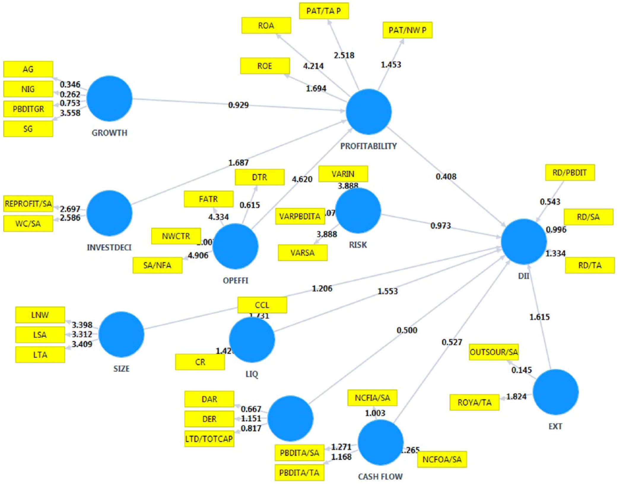
Final path diagram.

The values of latent construct DII are for the year 2013. The other latent constructs have variables with average values (2009-2012). The variable definitions are given in Table 1. The year t represents year 2013, t−1 is year 2012, and t−4 is year 2009. Descriptive statistics are presented in Appendix A.

Table 1.

Reflective and Formative Indicator Definitions.

	Variable definition
Latent construct DII
RD/TA	Research and development expenses in year t divided by total assets in year t
RD/SA	Research and development expenses in year t divided by total sales in year t.
ADVT/SA	Advertisement expenses in year t divided by sales in year t−1.
ADVT/TA	Advertisement expenses in year t divided by total assets in year t.
INTANG/SA	Intangible assets in year t divided by sales in year t.
RD/CAPEX	Research and development expenses in year t divided by capital expenditure in year t.
RD/PBDITA	Research and development expenses in year t divided by profit before depreciation, interest, taxes, and amortization in year t.
Latent construct GROWTH
AG	Average asset growth rate during period t−1 to t−4.
SG	Average sales growth rate during period t−1 to t−4.
NIG	Average net income growth rate during period t−1 to t−4.
PBDITGR	Average profit before depreciation interest and tax growth rate during period t−1 to t−4.
Latent construct RISK
VARIN	Variance of net income during the period t−1 to t−4.
VARSA	Variance of sales during the period t−1 to t−4.
VARPBDITA	Variance of profit before depreciation, interest, tax and amortization during period t−1 to t−4.
Latent construct CASH FLOW
PBDITA/SA	Profit before depreciation interest tax and amortization divided by sales (average values during period t−1 to t−4).
PBDITA/TA	Profit before depreciation interest tax and amortization divided by assets sales (average values during period t−1 to t−4).
NCFIA/SA	Net cash flow from financing activities divided by sales (average values during period t−1 to t−4).
NCFOA/SA	Net cash flow from operational activities divided by sales (average values during period t−1 to t−4).
Latent construct LIQ (liquidity)
CR	Current ratio: Current assets divided by current liabilities (average values t−1 to t−4).
CCL	Cash to current liabilities (average values t−1 to t−4).
Latent construct LEV (leverage)
DER	Debt to equity ratio (average values t−1 to t−4).
DAR	Debt to asset ratio (average values t−1 to t−4).
LTD/TOTCAP	Long-term debt to total capital employed (average values t−1 to t−4).
Latent construct INVESTDECI (investment policy in terms of capital expenditure and working capital)
CAPEX/SA	Capital expenditure/sales (average values t−1 to t−4).
REPROFIT/SA	Retained profits/sales (average values t−1 to t−4).
WC/SA	Working capital/sales (average values t−1 to t−4).
Latent construct PROFITABILITY
PBITDA/TN	Profit before interest, tax, depreciation and amortization divided by total income (average values t−1 to t−4).
NI/SA	Net income/sales (average values t−1 to t−4).
ROE	Net income divided by total net worth (average values t−1 to t−4).
ROA	Net income divided by total assets (average values t−1 to t−4).
PAT/TAP	Profit after tax divided by total assets (%; average values t−1 to t−4).
PAT/NWP	Profit after tax divided by net worth (%; average values t−1 to t−4).
PAT/TNP	Profit after tax divided by total income (%; average values t−1 to t−4).
Latent construct OPEFFI (asset utilization/efficiency ratios)
DTR	Debtor’s turnover ratio (average values t−1 to t−4).
NWCTR	Net working capital turnover ratio (net working capital/sales; average values t−1 to t−4).
FATR	Fixed assets turnover ratio (fixed assets/sales; average values t−1 to t−4).
SA/NFA	Sales/net fixed assets (average values t−1 to t−4).
Latent construct MARVAL (market valuations)^a
PE	Price earnings ratio (average values t−1 to t−4).
EPS	Earnings per share (average values t−1 to t−4).
Latent construct EXT (external factors)
ROYA/TA	Royalty payment/assets (average values t−1 to t−4).
OUTSOUR/SA	Outsourced expenses/sales (average values t−1 to t−4).
Latent construct SIZE
LSA	Log of sales (average values t−1 to t−4).
LTA	Log of assets (average values t−1 to t−4).
LNW	Log of net worth (average values t−1 to t−4).

Note. DII = discretionary investment intensity; RD = research and development; PLS-SEM = partial least squares structural equations modeling.

This construct was eliminated in the PLS-SEM final path.

Food Industry: A Snap Shot

India is the world’s second largest producer of food. The food processing industry is one of the largest industries in India and is ranked fifth in terms of production, consumption, export, and expected growth. The total food production in India is likely to double in the next 10 years with the country’s domestic food market estimated to reach US$258 billion by 2015 as per FRPT Research—Industry Updates, July 2014. Agriculture, which provides employment to 52% of the population, is estimated to account for 14% of the country’s GDP. Presently, the Indian food processing industry accounts for 32% of the country’s total food market. Agricultural & Processed food products Export Development Authority (APEDA) and Marine Products Export Development Authority (MPEDA) are the two agencies established by government of India for promotion of exports. The food industry in India has been attracting a lot of attention from foreign investors as the country is close to the markets of Middle East, Africa, and South East Asia. The food manufacturing industry is one of the United States’s largest manufacturing sectors, accounting for more than 10% of all manufacturing shipments. In 2013, the U.S. food and beverage manufacturing sector employed about 1.5 million people or just more than 1% of all U.S. non-farm employment. More than 31,000 food and beverage manufacturing plants are located throughout the country.

Expenditure on R&D is one of the most widely used measures of innovation inputs. R&D intensity is expressed as R&D expenditure as a percentage of GDP. Israel has the highest R&D intensity, with gross domestic expenditure on R&D (GERD) in excess of 4% of GDP.

R&D expenditure in the industrial sectors (both private and public) constitutes 30.4% of the total R&D expenditure of India. According to the Report of Research and Development Statistics (2008), industrial R&D expenditure was highest in the drug and pharmaceutical industry with a share of 37.4% of total R&D expenditures as compared with other industries.

In India, very few firms spend on R&D activities and its intensity is very low. In food product manufacturing industry, the 5-year average R&D intensity is 0.12. See Appendix B for industry wise R&D intensity in India. About 167 firms reported R&D expenses out of 1,150 firms. In terms of amount spent, ITC Limited leads in the food industry with 848.67 million Indian rupees, but in terms of R&D intensity (R&D/sales), ITC ranks very low at 50. In terms of research intensity, Green Earth Bio Tech leads in food industry with 34% followed by Venkateshwara Research & Breeding Farm Pvt. Limited with 33%. In terms of R&D intensity, small firms rank higher. See Tables 2 and 3, for example, though food major ITC tops in R&D expenses, it occupies a low ranking in terms of R&D intensity. This study provides unique results in terms of anomaly.

Table 2.

Top R&D Investor in Food Industry.

S. No.	Company	R&D (in million Indian rupees)
1	ITC Ltd.	848.67
2	NSL Sugars Ltd.	386.23
3	Maharashtra Hybrid Seeds Company Private Ltd.	347.27
4	GlaxoSmithKline Consumer Healthcare Ltd.	236.57
5	Venco Research & Breeding Farm Ltd.	174.95
6	Nestlé India Ltd.	137.74
7	Britannia Industries Ltd.	113.01
8	JK Agri Genetics Ltd.	112.10
9	Mondelez India Foods Private Ltd.	110.86
10	Dhampur Sugar Mills Ltd.	95.71
11	Godfrey Phillips India Ltd.	85.69
12	Venkateshwara Research & Breeding Farm Pvt. Ltd.	84.80
13	Monsanto India Ltd.	83.11

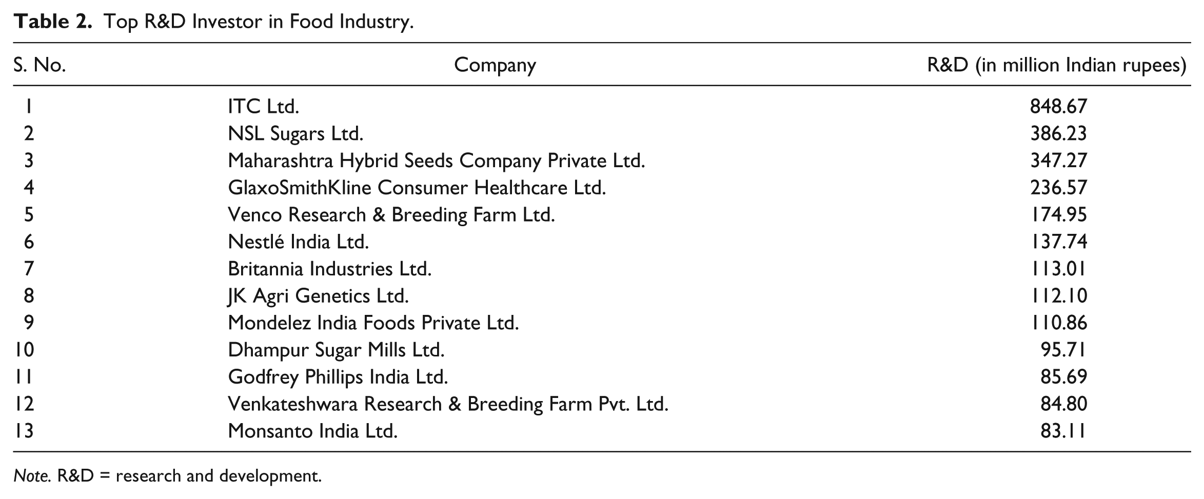
Note. R&D = research and development.

Table 3.

Rank Based on R&D Intensity.

Top companies in terms of R&D intensity
S. No.	Company	R&D/sales (in %)	R&D (in million Indian rupees)	Sales (in million Indian rupees)
1	Green Earth Bio Tech	34.27	5.60	16.34
2	Venkateshwara Research & Breeding Farm Pvt. Ltd.	32.67	84.80	259.60
3	Venco Research & Breeding Farm Ltd.	10.08	174.95	1,736.47
4	NSL Sugars Ltd.	9.65	386.23	4,003.02
5	Kasila Farms Ltd.	8.29	4.50	54.30
6	Maharashtra Hybrid Seeds Company Ltd.	8.15	347.27	4,260.22
7	Excel Genetics Ltd.	7.39	4.60	62.24
8	Unicorn Seeds Pvt. Ltd. [Merged]	7.26	12.08	166.50
9	Nath Bio-Genes (India) Ltd.	6.92	71.67	1,035.72
10	Advanta Ltd.	6.31	69.91	1,108.47
11	Metahelix Life Sciences Ltd.	6.14	32.73	532.88

Note. R&D = research and development.

Empirical Analysis

In PLS-SEM, the significance of factor loading is assessed by the bootstrapping procedure with minimum samples of 5,000 and the number of cases equivalent to sample size (n = 50). Bootstrapping is a non-parametric procedure which can be applied to test whether coefficients such as outer weights, outer loadings, and path coefficients are significant by estimating standard errors for the estimates. In the bootstrapping process, the subsamples are created with observations randomly drawn from the original data set (with replacement).

Through the process of bootstrapping, reflective and formative indicators which were not significantly loading with their respective loadings or not meeting the criteria were removed from the model. For reflective indicators, outer loading relevance testing is carried out based on the following criteria. If outer loading is less than 0.4, the reflective indicator is deleted. If the outer loading is less than 0.7 but greater than 0.4, then the impact of indicator deletion on AVE and the composite reliability are analyzed. If the deletion increases the measures above the threshold, the reflective indicator is deleted. If the measures already meet the threshold, then the reflective indicator is retained. The reflective indicators like NCFIA/SA (latent construct CASH FLOW); OUTSOUR/SA (latent construct EXT); AG, NIG, PBDITGR (latent construct GROWTH); DAR (latent construct LEV); and DTR (latent construct OPEFFI) were eliminated as their loadings were less than 0.4.

Validity Assessment of Reflective Measurement Models

The PLS-SEM algorithm has converged. The assessment of the reflective measurement model is done through indicator reliability, internal consistency reliability, convergent validity, and discriminant validity. The indicator reliabilities for reflective measures are analyzed by examining the outer loadings. Indicator reliability is also known as indicator communality. All the reflective indicators of latent construct RISK (VARIN, VARPBDITA, VARSA) were found to be statistically significant. All the reflective indicators of latent construct SIZE (LNW, LSA, LTA) were statistically significant. The reflective indicators of OPEFFI (FATR, SA/NFA, NWCTR); INVESTDECI (REPROFIT/SA,WC/SA);PROFITABILITY (PAT/TAP, ROA, ROE); EXT (ROYA/TA); and GROWTH (SG) were found to be statistically significant. On the basis of criteria for selection for reflective indicators with value between 0.4 and 0.7, the reflective indicator variable ROE was also deleted.

Table 4 shows the outer loadings of the indicator reliabilities after removal of the non-significant indicator variables. All the variables except RD/TA are reflective indicator variables. All reflective indicator variables are statistically significant. There is only one retained reflective variable in the latent construct EXT. Hence, its outer loadings are equal to 1. Similarly, there is only one formative indicator in the construct DII. DII refers to the measures of discretionary expenditures incurred by the sample of firms in the food industry. In this study, the discretionary expenses considered are the R&D measures. The initial formative variables used included RD/PBDIT, RD/SA, and RD/TA. In the final path construct, only the significant variable of RD/TA was found to be relevant and retained. Discretionary expenditures basically refer to advertising and R&D expenses. In the initial model, we included measures of advertising variables such as Advertisement/Sales and Advertisement/Total Assets. But the loading values were very low and insignificant.

Table 4.

Outer Loadings of Indicator Reliabilities.

	Original sample	Sample mean	p Value
CCL ← LIQ	0.986	0.959	.000
CR ← LIQ	0.779	0.841	.000
DER ← LEV	0.776	0.799	.000
FATR ← OPEFFI	0.909	0.890	.000
LSA ← SIZE	0.983	0.982	.000
LTA ← SIZE	0.982	0.982	.000
LTD/TOTCAP ← LEV	0.708	0.638	.000
NCFOA/SA ← CASH FLOW	0.717	0.591	.008
NWCTR ← OPEFFI	0.445	0.408	.034
PAT/NWP ← PROFITABILITY	0.599	0.647	.001
PAT/TAP ← PROFITABILITY	0.774	0.794	.000
PBDITA/SA ← CASH FLOW	0.606	0.646	.076
PBDITA/TA ← CASH FLOW	0.949	0.718	.003
RD/TA → DII	1.000	1.000
REPROFIT/SA ← INVESTDECI	0.936	0.920	.000
ROA ← PROFITABILITY	0.754	0.698	.000
ROYA/TA ← EXT	1.000	1.000
SA/NFA ← OPEFFI	0.787	0.785	.000
SG ← GROWTH	1.000	1.000
VARIN ← RISK	0.996	0.970	.000
VARPBDITA ← RISK	0.966	0.866	.000
VARSA ← RISK	0.995	0.969	.000
WC/SA ← INVESTDECI	0.551	0.531	.002

Note. DII = discretionary investment intensity.

Analysis of Internal Consistency of Reflective Indicators

The internal consistency reliability is analyzed through composite reliability and Cronbach’s alpha in Tables 5 and 6, respectively.

Table 5.

Composite Reliability.

Latent construct	Originals	Sample mean	p Value
CASH FLOW	0.809	0.684	.002
DII
EXT	1.000	1.000
GROWTH	1.000	1.000
INVESTDECI	0.729	0.719	.000
LEV	0.711	0.694	.000
LIQ	0.880	0.896	.000
OPEFFI	0.772	0.767	.000
PROFITABILITY	0.754	0.762	.000
RISK	0.991	0.952	.000
SIZE	0.982	0.982	.000

Note. DII = discretionary investment intensity.

Table 6.

Cronbach’s Alpha.

Latent construct	Original sample	Sample mean	p Value
CASH FLOW	0.759	0.755	.000
DII
EXT	1.000	1.000
GROWTH	1.000	1.000
INVESTDECI	0.364	0.360	.002
LEV	0.189	0.204	.070
LIQ	0.796	0.862	.000
OPEFFI	0.576	0.575	.000
PROFITABILITY	0.563	0.585	.000
RISK	0.986	0.916	.000
SIZE	0.964	0.963	.000

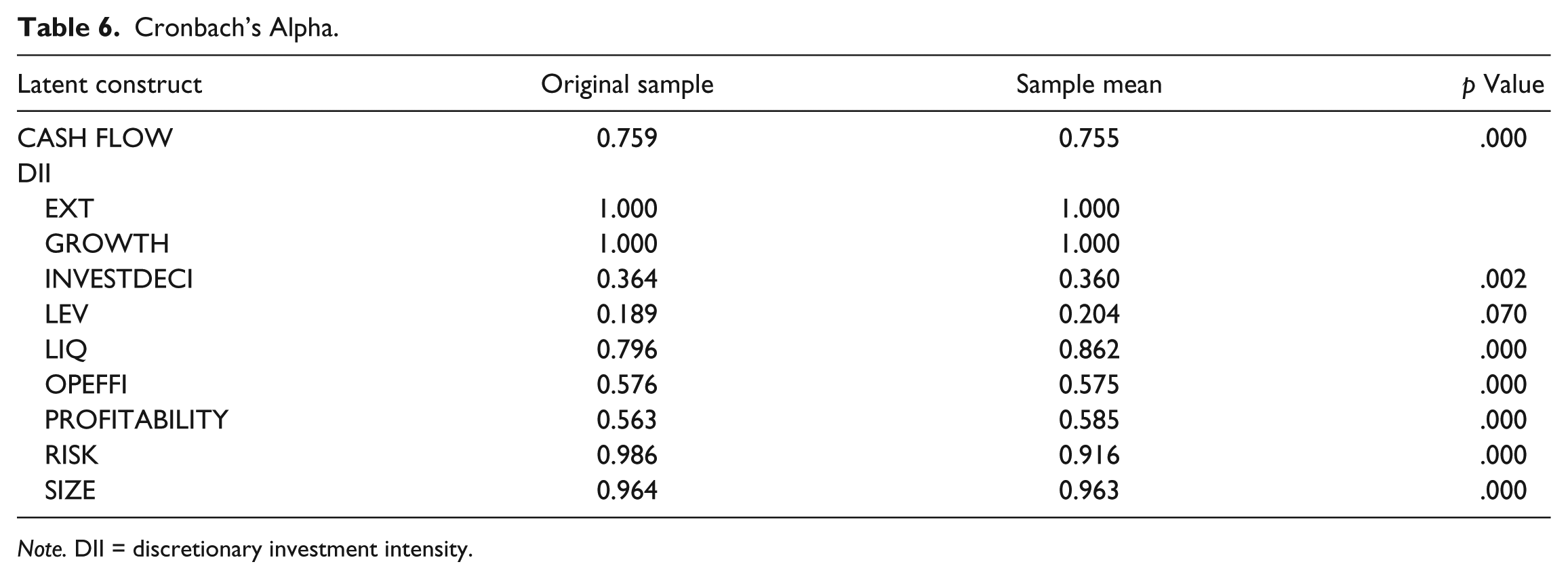
Note. DII = discretionary investment intensity.

Generally composite reliability values of greater than 0.6 are acceptable. The p values are statistically significant for all the latent constructs measuring growth, investment decisions, leverage, liquidity, operational efficiency, profitability, risk, size, and external factors. The latent construct EXT and GROWTH have reliability value of 1 as only one reflective indicator is present in the latent construct.

A Cronbach’s alpha measure of value 0.7 is considered reliable. Majority of the constructs have Cronbach’s alpha value greater than 0.7. The Cronbach’s alpha can be considered as the lower bound and the composite reliability as the upper bound of the true internal consistency reliability.

Measurement of Convergent Validity

The AVE is the measure of convergent validity. AVE is the grand mean of the squared loadings of all indicators associated with the construct. Each construct should account for at least 50% of the assigned indicators variance. It is also referred to as construct commonality. All the constructs satisfy the convergent validity criterion as shown in Table 7.

Table 7.

Average Variance Extracted.

Latent construct	Original sample	Sample mean	p Value
CASH FLOW	0.594	0.523	.001
DII
EXT	1.000	1.000
GROWTH	1.000	1.000
INVESTDECI	0.590	0.589	.000
LEV	0.552	0.550	.000
LIQ	0.789	0.831	.000
OPEFFI	0.548	0.555	.000
PROFITABILITY	0.509	0.537	.000
RISK	0.972	0.886	.000
SIZE	0.965	0.965	.000

Note. DII = discretionary investment intensity.

Each latent construct in the model has 50% or more of the assigned indicator variance.

Discriminant Validity

Discriminant validity is tested by means of assessment tests such as Fornell–Larcker criterion, cross loadings criterion, and the heterotrait-monotrait ratio of correlations (HTMT) as presented in Tables 8, 9, and 10, respectively.

Table 8.

Fornell–Larcker Criterion.

Latent construct	CASH FLOW	DII	EXT	GROWTH	INVEST	LEV	LIQ	OPEFFI	PROFIT	RISK	SIZE
CASH FLOW	0.771
DII	−0.136
EXT	0.124	0.224	1.000
GROWTH	0.300	−0.020	0.135	1.000
INVEST	0.586	−0.139	0.046	0.290	0.768
LEV	0.048	−0.157	−0.119	−0.039	−0.026	0.743
LIQ	0.031	0.339	0.238	0.014	0.103	−0.066	0.888
OPEFFI	0.249	0.023	0.048	0.290	0.152	−0.045	0.228	0.740
PROFIT	0.648	−0.110	0.180	0.373	0.502	−0.146	0.100	0.738	0.713
RISK	0.202	−0.054	−0.024	0.018	0.013	−0.062	−0.025	0.025	0.127	0.986
SIZE	0.335	−0.508	−0.026	0.064	0.248	0.184	−0.130	0.054	0.251	0.362	0.983

Note. DII = discretionary investment intensity.

Table 9.

Cross Loadings Criterion.

Latent construct	CASH FLOW	DII	EXT	GROWTH	INVESTDECI	LEV	LIQ	OPEFFI	PROFIT	RISK	SIZE
CCL	0.016	0.378	0.287	0.008	0.058	−0.055	0.986	0.224	0.087	−0.022	−0.117
CR	0.079	0.102	−0.013	0.033	0.24	−0.086	0.779	0.181	0.12	−0.03	−0.141
DER	−0.156	−0.123	−0.068	−0.119	−0.138	0.776	−0.094	−0.147	−0.286	−0.056	0.043
FATR	0.176	0.056	0.08	0.293	0.045	−0.05	0.191	0.909	0.733	0.015	0
LSA	0.368	−0.501	−0.012	0.098	0.26	0.173	−0.09	0.206	0.371	0.36	0.983
LTA	0.289	−0.498	−0.038	0.026	0.228	0.189	−0.165	−0.101	0.123	0.352	0.982
LTD/TOTCAP	0.251	−0.11	−0.11	0.072	0.113	0.708	0.001	0.094	0.089	−0.035	0.242
NCFOA/SA	0.717	−0.063	0.055	0.155	0.253	0.054	−0.04	−0.157	0.18	0.116	0.208
NWCTR	0.092	−0.019	−0.048	0.124	0.021	0.019	−0.079	0.445	0.254	0.031	0.128
PAT/NWP	0.422	−0.092	0.284	0.195	0.391	−0.267	0.059	0.138	0.599	0.081	0.244
PAT/TAP	0.866	−0.116	0.216	0.286	0.74	−0.091	0.146	0.288	0.774	0.192	0.359
PBDITA/SA	0.606	0.009	0.067	0.164	0.713	−0.011	−0.062	−0.218	0.215	0.135	0.304
PBDITA/TA	0.949	−0.139	0.133	0.311	0.654	0.034	0.052	0.366	0.732	0.205	0.338
RD/TA	−0.136	1	0.224	−0.02	−0.139	−0.157	0.339	0.023	−0.11	−0.054	−0.508
REPROFIT/SA	0.624	−0.035	0.129	0.292	0.936	−0.064	0.111	0.093	0.498	0.024	0.26
ROA	0.19	−0.049	0.004	0.296	0.068	−0.054	0.022	0.902	0.754	0.021	0.023
ROYA/TA	0.124	0.224	1	0.135	0.046	−0.119	0.238	0.048	0.18	−0.024	−0.026
SA/NFA	0.276	−0.016	0.021	0.19	0.27	−0.041	0.289	0.787	0.531	0.02	0.06
SG	0.3	−0.02	0.135	1	0.29	−0.039	0.014	0.29	0.373	0.018	0.064
VARIN	0.188	−0.057	−0.035	0.022	0	−0.063	−0.028	0.03	0.119	0.996	0.377
VARPBDITA	0.232	−0.041	0.007	0.006	0.049	−0.057	−0.017	0.009	0.143	0.966	0.302
VARSA	0.188	−0.057	−0.036	0.023	−0.001	−0.063	−0.028	0.031	0.119	0.995	0.378
WC/SA	0.143	−0.303	−0.179	0.111	0.551	0.078	0.021	0.2	0.21	−0.021	0.071

Note. DII = Discretionary investment Intensity.

Table 10.

Discriminant Validity Assessment Through Heterotrait-Monotrait Ratio.

	CASH FLOW	EXT	GROWTH	INVESTDECI	LEV	LIQ	OPEFFI	PROFIT	RISK
CASH FLOW
EXT	0.118
GROWTH	0.293	0.135
INVESTDECI	0.987	−0.054	0.427
LEV	0.12	−0.277	−0.073	0.063
LIQ	0.015	0.169	0.025	0.286	−0.192
OPEFFI	0.028	0.032	0.362	0.398	−0.071	0.271
PROFIT	0.805	0.307	0.472	1.059	−0.527	0.173	0.999
RISK	0.218	−0.022	0.017	0.008	−0.141	−0.031	0.038	0.182
SIZE	0.404	−0.026	0.065	0.357	0.45	−0.162	0.113	0.388	0.367

The Fornell–Larcker criterion suggests that the square root of AVE must be greater than the correlation of the construct with all other constructs including the formative measures in the structural model. The above criterion is satisfied with respect to all the constructs.

According to the cross loading criterion, each indicator must load highest on the construct in which it is an indicator measured both in terms of reflective and formative measures.

HTMT Criterion

HTMT is the average heterotrait-heteromethod correlations relative to the average monotrait-heteromethod correlations. Monotrait-heteromethod correlations represent correlations of indicators measuring the same construct. Heterotrait-heteromethod correlations are correlations of indicators across constructs measuring different phenomena. HTMT values close to 1 indicate lack of discriminant validity. The threshold value is considered close to 0.85. The constructs in this study satisfy the discriminant validity assessment on the basis of HTMT. The exception value is found for only construct profitability versus investment decision.

Validity Assessment of Formative Measurement Models

The validity assessment of formative measurement models consists of assessing the collinearity issues and assessment of significance and relevance of the formative indicators. Collinearity issues occur when two or more indicators of a construct are highly correlated. Collinearity assessment is done through the analysis of Variance Inflation Factors (VIFs). If there are no critical levels of collinearity (i.e., VIF < 5), then the assessment of formative measures enters the next stage.

Table 11 reveals that all VIF values are less than 5. The outer VIF values also satisfy the conditions of lack of multi-collinearity.

Table 11.

Collinearity Statistics Inner (VIF) Values.

	DII	PROFITABILITY
CASH FLOW	1.887
DII
EXT	1.101
GROWTH		1.170
INVESTDECI		1.098
LEV	1.137
LIQ	1.089
OPEFFI		1.098
PROFITABILITY	1.881
RISK	1.191
SIZE	1.358

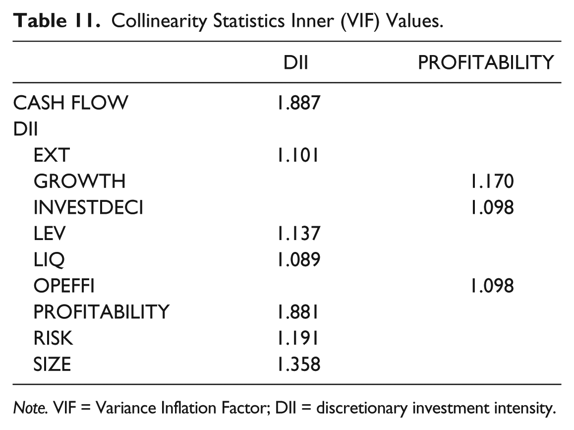
Note. VIF = Variance Inflation Factor; DII = discretionary investment intensity.

The next stage involves assessing the relevance of the formative indicators. The outer weight is assessed to be significant or not. If the outer weight is significant, then the operation is continued with the interpretation of the outer weight’s absolute and relative size. If the outer weight is not significant, then the formative indicator’s outer loading is analyzed. If the outer loading is less than 0.5, then the significance of the formative indicator’s outer loading is tested. If the outer loading is less than 0.5 and not significant, then the formative indicator is deleted. If the outer loading is less than 0.5 but is significant, then the removal of indicator may be considered. If the outer loading is greater than 0.5, then the indicator is retained even if it is not significant. Based on all these selection criteria, the only formative indicator which was included in the latent construct DII was RD/TA (research and development expenses / total assets). All other formative indicators representing advertising intensities and R&D intensities were deleted due to non-relevance based on selection criteria as discussed above.

Assessment of the Structural Model

The assessment of the structural model consists of five steps. In the first step, the structural model is assessed for collinearity issues. The VIF values are found to be less than 5. Hence, structurally the model does not have collinearity issues. The second step involves assessing the significance and relevance of the structural model relationships. The process involves testing the significance and relevance of path coefficients. The path coefficients vary between −1 and +1. The type of effects is divided into direct effects, indirect effect, and total effects. The third step involves examination of coefficient of determination R². R² is a measure of the model’s predictive accuracy. The fourth step involves measurement of effect sizes by means of F². The last step involves estimation of Q² to find the predictive relevance through blindfolding.

Path coefficient analysis explains the relevance and significance of path coefficients. Higher absolute values denote stronger predictive relationship between constructs. Direct effect measures the relationship linking two constructs with a single arrow between the two. Indirect effect measures the sequence of relationship with at least one intervening construct involved. The total effect is the sum of the direct effect and all indirect effects linking the two constructs.

The constructs signifying cash flow measures, externality (in terms of royalty measures), liquidity, and risk measures are directly and positively related to DII. The constructs signifying leverage and size are negatively related to DII. The relationship of risk and size with DII is statistically significant as shown in Table 12.

Table 12.

Path Coefficient Analysis.

	Original sample	Sample mean	SE	t Statistics (\|original sample / SE\|)	p Value
CASH FLOW → DII	0.029	0.078	0.216	0.133	.894
EXT → DII	0.163	0.128	0.120	1.356	.176
GROWTH → PROFITABILITY	0.072	0.055	0.052	1.376	.169
INVESTDECI → PROFITABILITY	0.381	0.423	0.134	2.846	.005
LEV → DII	−0.032	−0.062	0.065	0.497	.619
LIQ → DII	0.243	0.181	0.231	1.051	.294
OPEFFI → PROFITABILITY	0.659	0.615	0.138	4.768	.000
PROFITABILITY → DII	−0.077	−0.060	0.169	0.459	.647
RISK → DII	0.142	0.143	0.058	2.442	.015
SIZE → DII	−0.508	−0.512	0.137	3.696	.000

Note. DII = discretionary investment intensity.

The indicator variable values represent the average values for the period t−1 to t−4. The indicator variables for DII were for the period t. The path coefficient analysis reveals that higher the cash flow generation by the food sector firms, greater would be the R&D investments by the firm. But the results are not statistically significant. The royalty payments are directly related to R&D investments. This indicates that Indian firms in food industry use R&D efforts to adapt, assimilate, and develop imported technology. This result is similar to the findings of Katrak (1989) and Narayanan (1998). Firms with higher growth are more profitable. But the results do not show statistical significance.

The path coefficient for construct investment decisions (INVESTDECI) is 0.381 with statistical significance at all levels of significance. Higher the investments of the firms in terms of capital expenditures and working capital, higher is the profitability of the firms. Hence, the investment policy of the firms is a crucial determinant of the profitability of firms in food sector in India.

Leverage is negatively related to R&D intensity with no statistical significance. Higher the financial leverage of food sector firms, lower will be the investments in R&D. Firms with high leverage are considered to be riskier and hence such firms may not be proactive in R&D investments. Firms with higher liquidity positions would invest more in R&D. The results are not statistically significant in this case.

Food industry firms which are able to manage their assets efficiently are found to be more profitable. Higher the asset turnover ratios or asset management efficiency, higher is the profitability of firms. The path coefficient value of the original sample was 0.659 with statistical significance at 1% level.

The statistical significance of the relationship between profitability and R&D intensity is not established. Profitable firms may not focus much on R&D intensity.

The risk measures were analyzed through indicators representing variance of cash flow measures. The results suggest that riskier firms tend to invest much in R&D. It can be interpreted that riskier firms in food sector might focus on R&D investments as a strategy to generate more cash flows. The path coefficient value was 0.142 with statistical significance at 5% and 10% level.

Size is negatively related to R&D intensity. The path coefficient value was −0.508 with statistical significance at all levels. Smaller firms in food sector tend to invest more in R&D.

R² is a measure of the model’s predictive accuracy. It represents the amount of variance in the endogenous constructs explained by all of the exogenous constructs linked to it. The R² value for DII is 0.379 (see Table 13). It can be stated that all the exogenous variables used in the study accounts for 37.9% of variation in the in the endogenous construct DII. Similarly, about 70.5% of variation in profitability is explained by the exogenous variables associated with the construct.

Table 13.

R².

	Original sample	Sample mean	SE	T Statistics (\|original sample/SE\|)	p Value
DII	0.379	0.460	0.093	4.095	.000
PROFITABILITY	0.705	0.710	0.059	11.921	.000

Note. DII = discretionary investment intensity.

F² measures the size effects. It assesses how strongly one exogenous construct contributes to explaining a certain endogenous construct in terms of R². INVESTDECI to PROFITABILITY and OPEFFI to PROFITABILITY have strong effects (value greater than 0.35) and rest of the constructs have weak effects.

Blindfolding is an iterative procedure in which different parts of data matrix are omitted. The estimates based on the reduced data sets are used to predict the omitted parts. The prediction error is used as an indicator of predictive relevance. Q² value of 0.058 for DII signifies weak effect and 0.286 for PROFITABILITY signifies moderate effect.

Interpretation of Results

The study aims to analyze the impact of financial policies and firm characteristics on the discretionary investment strategy of the food industry firms. Using the PLS-SEM model, the study aims to understand the impact of financial policies on profitability and, in turn, its effect on the R&D investment strategy. Another focus of the article is to explore the impact of characteristics like size, leverage, risk, royalty, and outsourcing capabilities on the discretionary investment strategy of the firm. The investment policy decisions of firms in this sector are a major determinant of the profitability. The study finds that higher investments in the form of capital expenditures and working capital lead to higher profitability for firms in the food industry sector. It can be interpreted that firms in food industry sector would be able to enhance the profitability through sound capital investment decisions (selecting projects with positive NPV) and improving the working capital efficiency. Efficient management of assets also increases the profitability of the firms. However, the results could not establish the relationship between profitability and discretionary investment characteristics of food sector firms. The results do not show statistical significance to suggest that profitable firms invest more in R&D activities. Higher the risk, greater is the propensity to invest in R&D activities. Smaller firms tend to invest more in R&D activities (see Appendix C).

Conclusion and Implications

This study explores the determinants of discretionary expenses using PLS method. These determinants are considered as latent factors which can directly or indirectly influence the decision to invest in discretionary expenses. R&D and advertisement intensities are taken as discretionary expenses. In the initial analysis on account of low loading values which were insignificant, the advertising variable indicators were deleted from the discretionary investment construct.

Using PLS-SEM, the paths of these relationships are explored. This method allows to include different variables measuring latent factors. The result of the model shows that investment decision and operational efficiency are important factors which influence profitability. Manager’s ability to create value depends on the three major policy decisions involving investments, financing, and working capital management. The results of the study indicate that firms which invest in capital expenditure would create value for firms in form of increased profitability. Efficient asset utilization also emerges as a determinant of profitability of food sector firms. However, profitability turned out to be not influencing discretionary expenses. Riskier firms tend to invest more in discretionary expenses. It can be interpreted that investments in R&D itself is a risk-taking initiative for firms. Riskier firms in food sector might focus on R&D investments as a strategy to generate more cash flows. It is also interesting that size turned out to be negatively related to discretionary expenses. This study allows the managers to see the impacts of many variables representing latent factors which directly or indirectly influence their decision to invest on discretionary expenses. This allows the managers to pursue appropriate strategies for determining discretionary expenses.

Footnotes

Appendix A

Descriptive Statistics.

Variables	M	Median	SD	Minimum	Maximum
SG	0.716	0.490	1.076	−0.450	7.867
AG	279.287	0.361	1,990.510	−0.274	17119.867
NIG	5.124	0.484	42.525	−0.409	410.681
PBDITGR	1.815	0.684	6.137	−4.530	53.429
PBDITA/SA	0.131	0.121	0.083	−0.026	0.387
PBDITA/TA	0.143	0.119	0.101	−0.046	0.764
NCFIA/SA	−0.056	−0.038	0.067	−0.319	0.099
NCFOA/SA	0.056	0.047	0.076	−0.175	0.273
CR	1.747	1.041	4.247	0.384	38.838
CCL	0.418	0.075	1.824	0.006	16.093
DER	2.477	1.229	5.415	0.000	41.091
LTD/TOTCAP	19.387	9.382	25.819	0.026	129.493
DAR	0.361	0.381	0.231	0.000	0.845
CAPEX/SA	0.008	0.000	0.036	−0.012	0.257
REPROFIT/SA	0.027	0.022	0.058	−0.139	0.213
WC/SA	0.237	0.188	0.211	−0.239	0.786
PBITDA/TN	13.108	12.128	9.583	−2.610	75.154
NI/SA	1.016	1.011	0.086	0.288	1.226
ROA	1.345	1.036	0.846	0.409	4.927
ROE	25.020	3.613	202.219	−54.748	2,025.342
PAT/TNP	4.183	3.351	8.387	−13.608	50.194
PAT/NWP	6.952	13.201	40.540	−252.763	96.273
PAT/TAP	5.671	4.603	8.115	−12.781	36.798
DTR	32.824	19.383	51.409	1.444	427.331
NWCTR	7.340	4.688	23.372	−99.830	161.093
FATR	1.342	1.047	0.852	0.397	4.908
SA/NFA	6.824	4.038	7.715	0.708	44.012
EPS	66.397	8.793	968.756	−7,637.143	4,462.705
PE	11.752	10.482	31.713	−149.944	114.140
ROYA/TA	0.019	0.002	0.031	0.000	0.101
OUTSOUR/SA	0.015	0.009	0.019	0.000	0.083
LSA	8.716	8.517	1.061	7.204	12.686
LTA	8.593	8.498	1.157	6.457	12.513
LNW	7.307	7.221	1.526	−0.051	12.075
RD/SA	0.005	0.001	0.017	0.000	0.101
RD/TA	0.006	0.001	0.018	0.000	0.154
INTANG/SA	0.009	0.001	0.025	0.000	0.161
RD/PBDIT	0.041	0.008	0.175	−0.357	1.584

Note. RD = research and development.

Appendix B

Average R&D Intensity in Indian Manufacturing Sector.

S. No.	CMIE classification of industries	R&D/sales in %
1	Drugs and pharmaceuticals	4.647
2	Automobile	1.609
3	Alkalies (U)	1.109
4	Non-electrical machinery	0.865
5	Pesticides	0.825
6	Organic chemicals	0.82
7	Electronics	0.817
8	Paints and varnishes	0.609
9	Automobile ancillaries	0.586
10	Other chemicals	0.472
11	Rubber and rubber products	0.431
12	Dyes and pigments	0.397
13	Tobacco products	0.344
14	Cosmetics, toiletries, soaps, and detergents	0.278
15	Tyres and tubes	0.256
16	Inorganic chemicals	0.24
17	Polymers	0.222
18	Electrical machinery	0.2
19	Plastic products	0.189
20	Food products	0.124
21	Cement	0.103
22	Other non-metallic mineral products	0.085
23	Ferrous metals	0.078
24	Fertilizers	0.065
25	Petroleum products	0.064
26	Textiles	0.062
27	Non-ferrous metals	0.036

Note. R&D = research and development; CMIE = Center for Monitoring Indian Economy.

Appendix C

Declaration of Conflicting Interests

The author(s) declared no potential conflicts of interest with respect to the research, authorship, and/or publication of this article.

Funding

The author(s) received no financial support for the research and/or authorship of this article.

Author Biographies

K. S. Sujit is associate professor of economics at Institute of Management Technology, Dubai, UAE. He holds a PhD in economics from Hyderabad University, India. His areas of interest include Industrial organization, firm-level study of R&D, and advertisement and drivers of value creation in firm/sector.

B. K. Rajesh is professor of finance at Institute of Management Technology, Dubai, UAE. He received PhD from Indian Institute of Technology, Kharagpur, India. He has published several empirical research papers in reputed international journals and authored six books published by Academic Press Elsevier, USA; Palgrave Macmillan, UK; McGraw Hill, India; and ICFAI Books, India.

References

Arvanitis

(1997). The impact of firm size on innovative activity: An empirical analysis based on Swiss firm data. Small Business Economics, 9, 473-490.

Bain

J. S.

(1951). Relation of profit rate to industry concentration: American manufacturing, 1936-40. Quarterly Journal of Economics, 65, 293-324.

Barney

(1991). Firm resources and sustained competitive advantage. Journal of Management, 17, 99-120.

Clark

(2008). Marketing during a recession? Get the wind at your back. Retrieved from http://www.buzzmaven.com/2008/01/marketing-during-a-recession-get-the-wind-at-your-back.html

Cohen

W. M.

Levin

Mowery

(1987). Firm size and R&D intensity: A re-examination. Journal of Industrial Economics, 35, 543-563.

Del

M. A.

Papagni

(2003). R&D and the growth of firms: Empirical analysis of a panel of Italian firms. Research Policy, 32, 1003-1014.

Drucker

(1986, September). A crisis of capitalism. The Wall Street Journal, pp. 30-31.

George

M. Z.

Agnes Cheng

(1992). Marketing communication intensity across industries. Decision Sciences, 23, 758-769.

Graham

Kristina

(2008). The earnings effects of advertising expenditures during recessions. New York, NY: American Association of Advertising Agencies.

10.

Grullon

George

(2006). The impact of capital structure on advertising competition: An empirical study. Journal of Business, 79, 3101-3124.

11.

Guariglia

(2008). Internal financial constraints, external financial constraints, and investment choice: Evidence from a panel of UK. Journal of Banking & Finance, 32, 1795-1809.

12.

Haenlein

Kaplan

A. M.

(2004). A beginner’s guide to partial least squares analysis. Understanding Statistics, 3, 283-297.

13.

Hair

J. F.

Jr. Hult

G. T. M.

Ringle

C. M.

Sarstedt

(2014). A primer on Partial Least Squares Structural Equation Modeling (PLS-SEM). Thousand Oaks, CA: SAGE.

14.

Henry

John

(2000). The determinants of pharmaceutical research and development expenditures. Journal of Evolutionary Economics, 10, 201-215.

15.

Hirsch

Gschwandtner

(2013). Profit persistence in the food industry: Evidence from five European countries. European Review of Agricultural Economics, 40, 741-759.

16.

Hirsch

Hartmann

(2014). Persistence of firm-level profitability in the European dairy processing industry. Agricultural Economics, 45, 53-56.

17.

Y. K.

Mira

Chee

M. Y.

(2006). Size, leverage, concentration, and R&D investment in generating opportunities. Journal of Business, 79, 851-876.

18.

Hovakimian

(2009). Determinants of investment cash flow sensitivity. Financial Management, 38, 161-183.

19.

Jacobs

(1991). Short-term America: The causes and cures of our business myopia. Boston, MA: Harvard Business School Press.

20.

Jensen

M. C.

(1986). Agency costs of free cash flow, corporate finance, and takeovers. The American Economic Review, 76, 323-329.

21.

Jensen

M. C.

William

H. M.

(1976). Theory of the firm: Managerial behavior, agency costs and ownership structure. Journal of Financial Economics, 3, 305-360.

22.

Kamber

(2002). The brand manager’s dilemma: Understanding how advertising expenditures affect sales growth during a recession. Journal of Brand Management, 10, 106-121.

23.

Katrak

(1989). Imported technologies and R&D in a newly industrializing country: The experience of Indian enterprises. Journal of Development Economics, 31, 123-139.

24.

Kotabe

(1990). The relationship between offshore sourcing and innovativeness. Journal of International Business Studies, 21, 623-639.

25.

Lee

Sung

(2005). Schumpeter’s legacy: A new perspective on the relationship between firm size and R&D. Research Policy, 34, 914-931.

26.

Long

M. S.

Ileen

B. M.

(1983). Investment patterns and financial leverage. In Friedman

B. M.

(Ed.), Corporate capital structures in the United States (pp. 353-377). Chicago, IL: University of Chicago Press.

27.

Mason

E. S.

(1939). Price and production policies of large scale enterprises. The American Economic Review, 29, 61-74.

28.

Michael

J. M.

(2005). Does being R&D intensive still discourage outsourcing? Evidence from Dutch manufacturing. Research Policy, 34, 571-582.

29.

Myers

S. C.

(1977). Determinants of corporate borrowing. Journal of Financial Economics, 5, 147-176.

30.

Narayanan

(1998). Technology acquisition, de-regulation and competitiveness: A study of Indian automobile industry. Research Policy, 27, 215-228.

31.

Nishimura

K. G.

Takanobu

Kozo

(2005). Does the natural selection mechanism still work in severe recessions? Examination of the Japanese economy in the 1990s. Journal of Economic Behavior & Organization, 58, 53-78.

32.

Paunov

(2012). The global crisis and firms’ investments in innovation. Research Policy, 41, 24-35.

33.

Petter

Straub

Rai

(2007). Specifying formative constructs in information systems research. MIS Quarterly, 31, 623-656.

34.

Porter

(1992). Capital choices: Changing the way America invests in industry. Boston, MA: Council on Competitiveness.

35.

Raji

Gary

L. L.

Shrihari

(2011). Should firms spend more on research and development and advertising during recessions? Journal of Marketing, 75, 49-65.

36.

Rigdon

E. E.

(1998). Structural equation modeling. In Marcoulides

G. A.

(Ed.), Modern methods for business research (pp. 251-294). Mahwah, NJ: Lawrence Erlbaum.

37.

Ryan

Wiggins

(2002). The interactions between R&D investment decisions and compensation policy. Financial Management, 31, 5-29.

38.

Schumpeter

(1961). Theory of economic development. New York, NY: Oxford University Press.

39.

Siddharthan

(1992). Transaction costs, technology transfer and in-house R&D: A study of the Indian private corporate sector. Journal of Economic Behavior & Organization, 18, 265-271.

40.

Srinivasan

Gary

L. L.

Arvind

(2005). Turning adversity into advantage: Does proactive marketing during a recession pay off? International Journal of Research in Marketing, 22, 109-125.

41.

Valarie

A. Z.

Rajan

P. V.

Carl

P. Z.

(1988). The contingency approach: Its foundations and relevance to theory building and research in marketing. European Journal of Marketing, 22(7), 37-64.

42.

Wernerfelt

(1984). A resource-based view of the firm. Strategic Management Journal, 5, 71-80.

43.

Wong

K. K. K.

(2013). Partial Least Squares Structural Equation Modeling (PLS-SEM) techniques using SmartPLS (Marketing Bulletin, 2013, 24, Technical Note 1). Retrieved from https://www.researchgate.net/file.PostFileLoader.html?id=55d6fbae5dbbbdb3608b45e0&assetKey=AS%3A273837248188417%401442299297149

Determinants of Discretionary Investments

Abstract

Keywords

Introduction

Review of Literature

Theoretical Postulates

Data, Sample, and Method

Method

Model Specification

Food Industry: A Snap Shot

Empirical Analysis

Validity Assessment of Reflective Measurement Models

Analysis of Internal Consistency of Reflective Indicators

Measurement of Convergent Validity

Discriminant Validity

HTMT Criterion

Validity Assessment of Formative Measurement Models

Assessment of the Structural Model

Interpretation of Results

Conclusion and Implications

Footnotes

Appendix A

Appendix B

Appendix C

Declaration of Conflicting Interests

Funding

Author Biographies

References